Sharif University of Technology
Scientia IranicaTransactions E: Industrial Engineering http://scientiairanica.sharif.edu
A variable iterated greedy algorithm based on grey
relational analysis for crew scheduling
K. Peng
a,band Y. Shen
a,b;a. School of Automation, Huazhong University of Science and Technology, Wuhan 430074, China.
b. Key Laboratory of Image Processing and Intelligent Control (Huazhong University of Science and Technology), Ministry of Education, China.
Received 14 May 2015; received in revised form 24 August 2016; accepted 4 Mar 2017
KEYWORDS Public transit; Crew scheduling; Variable iterated greedy;
Grey relational analysis; Local search.
Abstract. Public transport crew scheduling is a worldwide problem, which is NP-hard. This paper presents a new crew scheduling approach, called GRAVIG, which integrates Grey Relational Analysis (GRA) into a Variable Iterated Greedy (VIG) algorithm. The GRA is utilized as a solver for shift selection during the schedule construction process, which can be considered as a Multiple Attribute Decision Making (MADM) problem, since there are multiple static and dynamic criteria governing the eciency of a shift to be selected into a schedule. Moreover, in the GRAVIG, a biased probability destruction strategy is elaborately devised to maintain the `good' shifts in the schedule without compromising the randomness. Experiments on eleven real-world crew scheduling problems show that the GRAVIG can generate high-quality solutions close to the lower bounds obtained by the CPLEX in terms of the number of shifts.
© 2018 Sharif University of Technology. All rights reserved.
1. Introduction
The crew scheduling problem is one of the important components of the public transit operations planning process [1]. It is concerned with nding the most ecient way of partitioning vehicle work into a crew schedule. Ecient schedules can make signicant monetary savings for transportation operators since crew wages are a very large cost element of public transport operations [2-4].
To clarify the problem, some terminologies are rst introduced. A shift is the work that a crew carries out in a day, and it must satisfy a set of predened operational constraints and labor rules, e.g., the time for a crew to work without a meal break has to be
*. Corresponding author. Tel.: +86 27 87540055; Fax: +86 27 87543130
E-mail addresses: [email protected] (K. Peng); [email protected] (Y. Shen)
doi: 10.24200/sci.2017.4434
limited to a given number of hours. A schedule is dened as a solution to the problem that contains a set of shifts that cover all the vehicle work. Vehicle work is usually presented by a set of blocks. A block presents a sequence of vehicle work to be operated by one vehicle during a day. An example of a block is illustrated in Figure 1.
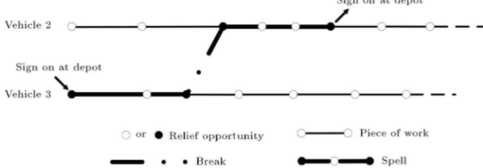
A Relief Opportunity (RO) is a pair of time and place where a crew can be relieved for reasons such as having a meal break and changing vehicle. Not all ROs will be actually used to relieve crews. The individual period between any contiguous pair of ROs on the same vehicle is called a piece of work (piece for short). A spell is constituted by a set of successive pieces on a vehicle. A shift contains one or more (at most four in general) spells with breaks in between, starting and ending with a sign-on and a sign-o at a depot. A two-spell shift is illustrated in Figure 2.
Crew scheduling is the process of compiling a schedule with smallest number of shifts and least cost. Meanwhile, each shift must be feasible, and each piece
Figure 1. An example of a block.
must be assigned to a shift. The problem is NP-hard and has attracted much research interest since 1960's [5]. Many crew scheduling approaches have been proposed in a series of international conferences (e.g., [6]). Since 1990's, metaheuristics have been widely used to solve the problem. The major classes in-clude Genetic Algorithm [7-11] and Tabu Search [7,12-14]. Other metaheuristics have also been employed, e.g. Variable neighborhood search [15], simulated anneal-ing [16], self-adjustanneal-ing approach [17], greedy random-ized adaptive search procedure [15,18], squeaky wheel optimization [19], and ant colony optimization [20].
In many crew scheduling approaches, e.g. [9,11,17,19], shift evaluation methods are essential, which decide the quality of schedule compilation. The most straightforward shift evaluation methods are sin-gle criterion-based, i.e. evaluating a shift based on an evaluation criterion. However, the solution qualities of the greedy heuristics with such evaluation methods have been proven unacceptable [17,21]. Later, multiple criteria-based evaluation methods have been proposed, which evaluate a shift comprehensively in light of multiple criteria. For example, in [9], the authors presented a genetic algorithm with fuzzy evaluation for crew scheduling, in which a fuzzy shift evaluation method was devised based on fuzzy set theory; In [22], the authors proposed an evolutionary algorithm based on Grey Relational Analysis (GRA), where a shift eval-uation method based on GRA was devised and its pa-rameters were obtained by a hybrid genetic algorithm. This paper proposes a new crew scheduling ap-proach, called GRAVIG, which integrates GRA into a Variable Iterated Greedy (VIG) algorithm. The VIG is a metaheuristic that has been successfully applied to solve a variety of combinatorial optimization problems such as traveling salesman problem with time windows [23-25], which is composed of ve phases: ini-tialization, destruction, construction, local search, and acceptance criterion. Applying the VIG for the crew scheduling problem, shift selection plays an essential
role during the schedule construction and destruction processes. The GRAVIG employs the GRA as a solver for the shift selection, which can be considered as a Multiple Attribute Decision Making (MADM) problem, since there are multiple static and dynamic criteria governing the eciency of a shift to be selected into or removed from a schedule. Moreover, in the GRAVIG, a biased probability destruction strategy is elaborately devised to maintain the `good' shifts in the schedule without compromising the randomness. The GRAVIG can be classied as the Generate and Select (GaS) approach. The GaS approach rst generates a large set of shifts satisfying all the given operational constraints and labor rules (called generation phase), from which a subset is selected to form the schedule (called selection phase).
The rest of the paper is organized as follows. The formulation of the crew scheduling problem is presented in Section 2. The shift evaluation method based on GRA is described in Section 3. The details of the proposed GRAVIG are then presented in Section 4. Ex-perimental results on real-world problems are displayed in Section 5. Finally, concluding remarks are given in Section 6.
2. Formulation of the crew scheduling problem Given m pieces P = fp1; p2; :::; pmg and n shifts S =
fS1; S2; :::; Sng, where each shift Sj covers a subset of
pieces, the crew scheduling problem can be formulated as the following set covering problem:
Minimize Xn
j=1
(C + cj)xj; (1)
Subject to
n
X
j=1
aijxj 1; 8i 2 f1; 2; :::; mg; (2)
xj = 0 or 1; 8j 2 f1; 2; :::; ng; (3)
where xj = 1 if Sjis selected, otherwise xj= 0; aij = 1
if Sj covers piece pi, otherwise aij = 0; cj is the cost of
Sj, and C is a large constant.
Eq. (1) minimizes the number of shifts selected and corresponding shift cost, where minimizing the number of shifts has priority over minimizing the shift cost; Relation (2) ensures that each piece is covered by at least a shift; and Eq. (3) assures that all the shifts are considered. The quality of a schedule is attributable to the number of shifts included and the cost of each component shift.
3. A shift evaluation method based on GRA Given a crew scheduling with n shifts, S = fS1; S2;
:::; Sng, a schedule with minimal number of shifts and
shift cost is to be constructed. Shift selection plays an important role. Such a shift selection problem can be considered as an MADM problem, since there are multiple static and dynamic criteria governing the eciency of a shift to be selected into a schedule.
GRA is one of the most important components of grey system theory [26-28]. It belongs to the family of MADM methods, which select the best from the exist-ing alternatives by considerexist-ing multiple criteria [29,30]. In this paper, GRA is employed for the shift selection during the schedule construction process.
GRA is an impact evaluation model that mea-sures the degree of similarity or dierence between two comparability sequences based on the grade of relation. A comparability sequence consists of the performances evaluated by each criterion in the given set of criteria. Given a set of comparability sequences, an ideal target sequence can be easily generated, called reference sequence. The basic principle of GRA is that a comparability sequence is regarded as the best if it has the highest grey relational grade with the reference sequence.
Tailoring GRA for the shift selection, a dynamic criterion and ve static criteria, i.e. working time (C1), ratio of working time over wage cost (C2),
number of pieces (C3), number of spells (C4), and
value in the relaxed LP solution (C5), are considered.
The values of the ve static criteria for each shift Sj 2 S are called a performance sequence, denoted
by Yj = (yj(1); yj(2); yj(3); yj(4); yj(5)), according to
which the comparability sequence is rst obtained and then the reference sequence is dened. Finally, the grey relational grade between the comparability sequence and reference sequence is calculated, which is called static evaluation. Moreover, the dynamic criterion is measured by the over-cover of pieces by shifts and called dynamic evaluation, which reects how well it ts the other shifts in the schedule. A comprehensive evaluation based on the two parts is devised.
3.1. Static evaluation 3.1.1. Grey relational generating
Grey relational generating is to transform the
performance sequence of each shift into a comparability sequence.
Criteria C1, C2, C3, and C5 belong to the
larger-the-better criteria, since a shift with larger yj(k) (k = 1; 2; 3; 5) is generally regarded better,
while C4 belongs to the
closer-to-the-desired-value-the-better criteria, because a shift with 2 spells is always considered better, i.e. the desired value is 2. Yj is transformed into a comparability sequence,
Xj = (xj(1); xj(2); xj(3); xj(4); xj(5)), by employing
the following Eqs. (4) and (5), where xj(k) is in the
range [0,1]:
xj(k) =
yj(k) minj yj(k)
max
j yj(k) minj yj(k)
;
j = 1; 2; :::; n; k = 1; 2; 3; 5; (4)
xj(k) = 1 jyj(k) 2j
max
max
j yj(k) 2; 2 minj yj(k)
;
j = 1; 2; :::; n; k = 4: (5) 3.1.2. Reference sequence
After obtaining the comparability sequences for all the shifts, reference sequence X0 = (x0(1); x0(2); x0(3);
x0(4); x0(5)) can be dened by setting x0(k) =
maxfxj(k)jj = 1; 2; :::; ng; k = 1; 2; :::; 5. Therefore,
X0= (1; 1; 1; 1; 1) corresponds to the articial shift S0.
3.1.3. Grey relational coecient
A grey relational coecient (denoted as (x0(k);
xj(k))) is the foundation for calculating the grey
relational grade between Xj and X0 according to the
kth criterion. It is calculated by Eq. (6): (x0(k); xj(k)) = jx min+ max
0(k) xj(k)j + max
j = 1; 2; :::; n; k = 1; 2; 3; 4; 5; (6) where min = minj mink jx0(k) xj(k)j, max = maxj
max
k jx0(k) xj(k)j, 2 [0; 1] is the distinguishing
coecient, and usually = 0:5. 3.1.4. Grey relational grade
Grey relational grade between Xj and X0, denoted as
(x0; xj), is calculated by Eq. (7):
(x0; xj) = 5
X
k=1
wk(x0(k); xj(k)); (7)
where wk (wk 0) denotes the weight of criterion Ck
andP5k=1wk= 1.
3.1.5. Static evaluation functions
for shift Sj, denoted as f(Sj), i.e.:
f(Sj) = (x0; xj): (8)
Moreover, relative grey relational grade, which inte-grates the ideas of GRA and TOPSIS, is suggested to be used as the static evaluation function, and it is dened as follows:
f(Sj) =(x (x0; xj)
0; xj) + (x0; xj); (9)
where (x0; x
j) denotes the grey relational grade
between Xj and the negative ideal sequence
X0 = (x0(1); x0(2); x0(3); x0(4); x0(5)), and x0(k) =
minfxj(k)jj = 1; 2; :::; ng.
3.2. Comprehensive evaluation
Dynamic evaluation function, denoted by g(Sj), is
realized by measuring cover of pieces, where over-cover means a piece is over-covered by more than one shift. It is dened in Eq. (10):
g(Sj) = jSjj
X
k=1
(jk jk)
,jSjj X
k=1
jk; (10)
where jSjj denotes the number of pieces in Sj, and jk
is the working time of piece k in Sj:
jk=
(
0; if piece k in Sj is covered
1; otherwise (11) Based on the static evaluation function and dynamic evaluation function, comprehensive evaluation function is devised in Eq. (12):
F (Sj) = (f(Sj)) (g(Sj)); j = 1; 2; :::; n; (12)
where ; 2 [0; 1] reects the relative inuence of the static evaluation and dynamic evaluation.
4. The GRAVIG approach
The VIG only provides a general framework, which should be elaborately tailored for solving dierent com-binatorial optimization problems. To solve the crew scheduling problem, this section proposes the GRAVIG approach, which considerably enhances the VIG by integrating with GRA. The GRA is employed in the initialization, construction, and destruction processes, aimed at selecting the most suitable shifts to construct or destruct a schedule. Such a shift selection problem can be regarded as an MADM problem, where multiple criteria are applied. The GRAVIG also devises a biased probability destruction replacing the traditional random destruction, which is able to maintain the `good' shifts in the schedule without compromising the randomness. The details of the GRAVIG are described below.
4.1. Initialization
To construct an initial schedule X0, the GRA is
employed to decide which shifts will be used: The higher the evaluation value of a shift, the higher the desirability of using it in the schedule will be, which is described as follows:
1. Set the initial schedule, X0= ;
2. For each piece pi2 P , build a coverage list, denoted
as Li, which contains all the shifts covering pi; then,
sort the pieces by the size of their coverage list in ascending order;
3. For the piece pi 2 P , nd the shift Sk 2 Li
satisfying F (Sk) = maxfF (Sj)jSj 2 Lig and set
X0= X0[ fS
kg and P = P fSkg;
4. Output X0.
4.2. Biased probability destruction
In the biased probability destruction, the current sched-ule (say X1) is destructed by removing d shifts, where
d is called destruction size. We devise a biased probability selection to achieve this: Evaluate the shifts in X1 by the GRA rst, sort them by the evaluation
values in ascending order, and then select d dierent shifts according to a biased probability distribution, where the shift of rank i is selected with probability Pi:
Pi= i jXP1j
i=1i
; (13)
where is a positive real number and we set = 1:2 in this paper. A shift with a higher evaluation value will have lower probability to be removed, i.e. the `good' shifts have higher probability of being maintained in the schedule. This is dierent from the canonical VIG, where the worst or randomly selected elements are to be removed.
The initial destruction size is set as dmin, and then
d adjusts adaptively within a range [dmin; dmax] (called
destruction size range), where dmin and dmax denote
minimum and maximum destruction sizes, respectively. At each iteration, if d becomes larger than dmaxor the
solution is better than the best solution found so far, set d = dmin; otherwise, add 1 to d. This is dierent
from the canonical VIG, where d is set to be dmin if d
is larger than dmax or the solution obtained is better
than the current solution. Moreover, the destruction size range may inuence the quality of the nal results, since a small value of d will make it dicult for the GRAVIG approach to escape from local optima while a large value of d will make this destruction procedure similar to a randomized procedure. Diering from the canonical VIG, where the destruction size range is usually set to be [1; N], in this paper, we set the
destruction size range to be [aN; bN] (0 < a < b <
1), where N is the number of shifts in the current schedule minus one, a and b are set to be 0.1 and 0.4, respectively.
4.3. Construction
In the destruction, d shifts are removed. The obtained partial schedule is denoted as X2. Consequently, the
pieces, which are covered by the d shifts exclusively, become uncovered. To cover them, the GRA is employed to determine which shifts should be selected. The major steps are as follows:
1. Set U = fthe pieces which are uncoveredg;
2. For each piece, pi 2 U, build a coverage list,
denoted as Li, which contains all the shifts covering
pi; then, sort the pieces by the size of their coverage
list in ascending order;
3. For the piece pi 2 U, nd the shift Sk 2 Li with
F (Sk) = maxfF (Sj)jSj2 Lig, and set X2= X2[
fSkg, U = U fSkg;
4. Output X2.
4.4. Local search
To further improve the new schedule, X2, generated
by the construction, a local search is employed, which focuses on removing redundant shifts and replacing shifts. A shift is dened as redundant if all of its pieces can be covered by the other shifts in the schedule. The local search contains the following steps:
1. Sort the shifts in X2by cost in descending order;
2. Delete the redundant shifts in X2;
3. Check each shift in X2 in descending order: If
it is a redundant shift, then delete it; otherwise, if it can cover k (1 k 3) pieces exclusively, replace it with a shift Sj =2 X2, which can cover k
pieces and has the lowest cost. If any of the above two conditions occurs, re-execute step 3; otherwise, terminate and output X2.
It should be mentioned that the parameter k = 3 in the local search is only implemented for the best schedule produced by the GRAVIG. The purpose is to achieve a tradeo between less CPU time and better results.
4.5. Acceptance criterion
The new schedule should be evaluated and it should be decided whether it is acceptable. We adopt a acceptance criterion as follows: The new schedule X2
replaces the original schedule X1 with the probability
min(1; e (G(X2) G(X1))/T
), where G(X1) and G(X2)
denote the costs of X1 and X2, respectively, i.e.:
G(X1) = X Sj2X1
(C + cj);
G(X2) = X Sj2X2
(C + cj):
T is the temperature at the current iteration, which decreases according to a proportional temperature cooling schedule, i.e. T = cT , where c is set to be 0.9 in this paper.
4.6. Framework of the GRAVIG approach Let T0 denote an initial temperature, M denote the
maximum number of iterations at the current tem-perature T , and N denote the maximum number of iterations for the GRAVIG; the framework of the GRAVIG is presented as follows:
1. Generate an initial schedule X0 by initialization
and improve it by local search; then, obtain a new schedule, X1, set the best schedule X= X1;
2. Set n = 0 and T = T0;
3. Initialize the destruction size range by setting dmin= jX1ja and dmax= jX1jb, and set d = dmin;
4. Improve X1 by M iterations at the temperature
T , and update X, which can be illustrated by the
following steps:
4.1 Set m = 0;
4.2 Generate a new schedule, X2, by sequentially
employing biased probability destruction and construction, and then improve it by local search;
4.3 If X2 is better than X, i.e. G(X2) < G(X),
set X = X2, d = dmin; otherwise, set d =
d + 1;
4.4 Set X1 = X2 if acceptance criterion is
satis-ed;
4.5 Update the values of dminand dmaxby setting
dmin = jX1ja and dmax = jX1jb, and if d is
out of the destruction size range [dmin; dmax],
set d = dmin;
4.6 Set m = m + 1 and n = n + 1;
4.7 If m < M, go to step 4.2.
5. Decrease T by setting T = cT ;
6. If the termination condition has been met (e.g. n N), improve Xusing local search, and then output
X; otherwise, go to step 4.
5. Computational results
The major concern about using heuristics is the quality of the obtained solution. In this paper, to evaluate the
Table 1. Size of test instances. Data Number of
blocks
Number of pieces
Number of shifts
BT08 8 184 14218
WH5 14 162 9714
ZJQZ2 18 491 31712
WJ302 30 389 74864
ZH40 40 528 31493
HS9 43 302 48267
HK4 46 467 97386
BJ41 54 410 55977
GZBM 30 750 93853
GZHD 49 584 137355
SY40 62 830 112142
eciency of the proposed GRAVIG, we have carried out experiments on 11 crew scheduling instances, which are derived from real-world problems in China. Their characteristics are shown in Table 1.
The GRAVIG is coded in C++ and implemented on a 2.60 GHz PC with 992M RAM under Windows XP, while the CPLEX 12.4 is run on a 2.13 GHz PC with 2GB RAM under Windows 7. The parameters are set as follows: T0 = 100, N = 700, M = 100,
= 0:5, (; ) = (1:0; 1:0), and (w1; w2; w3; w4; w5) =
(0:15; 0:15; 0:15; 0:15; 0:4), which is a good parameter Li and Kwan [9].
For comparison purpose, the benchmark exper-imental results in terms of shift number and total cost are conducted by comparing the GRAVIG with
CPLEX 12.4. Moreover, computational experiments are also conducted by comparing the GRAVIG with the following 3 algorithms: a recently proposed crew scheduling approach, i.e. Adaptive Evolutionary Crew Scheduling (AECS) approach in [11], the VIG, and an Iterated Greedy (IG) algorithm. This paper applies Relative Percentage Deviation (RPD) to the results of CPLEX, AECS, VIG, and IG to measure the performance of the GRAVIG, where:
RPD =
GRAVIG0s result A0s result
A0s result
100%;
where A denotes CPLEX, AECS, VIG, or IG.
5.1. Comparison of the GRAVIG with CPLEX The average results of 10 independent runs for the GRAVIG are reported in Table 2, where the results of CPLEX are also given. Columns 2-4 list the results of CPLEX in terms of shift number, shift cost, and elapsed time, respectively, where `{' denotes that integer solution cannot be found by CPLEX. For comparison purpose, we further calculate the lower bound of the number of shifts in an optimal schedule by employing CPLEX to solve the LP relaxation of the crew scheduling model, i.e. Eqs. (1)-(3) in Section 2; the corresponding results are listed in the 5th column of Table 2. The remaining columns report the results of the GRAVIG and its comparison with CPLEX.
From Table 2, it can be seen that for the rst 8 instances, CPLEX can nd the integer solution, and the average RPDs of the GRAVIG over the CPLEX are 1.28% and 9.86% in terms of shift number and
Table 2. Comparative results for CPLEX and GRAVIG.
Data CPLEX's solution Lower bound GRAVIG' s schedule # of
shifts Cost (hours)
Time (sec.)
# of shifts
# of shifts
RPDa
(%)
RPDb
(%)
Cost (hours)
RPDa
(%) Time (sec.)
BT08 23 139.43 16 23 23 0 0 156.19 12.0 9.9
WH5 21 151.15 5 21 22 4.76 4.76 156.61 3.61 6.5
ZJQZ2 31 221.37 30 31 32 3.23 3.23 235.57 6.41 36.9
WJ302 44 292.12 41 44 45 2.27 2.27 316.96 8.50 45.1
ZH40 64 380.85 24 64 64 0 0 425.27 11.67 25.1
HS9 68 439.88 43 68 68 0 0 448.36 1.93 21.2
HK4 70 448.77 94 70 70 0 0 491.87 9.60 51.5
BJ41 99 588.33 43 99 99 0 0 736.06 25.11 24.2
GZBM { { { 60 60.2 { 0.33 452.00 { 67.5
GZHD { { { 85 85.9 { 1.06 655.26 { 65.1
SY40 { { { 83 84.2 { 1.45 599.25 { 73.6
Avg. RPDc 1.28 1.19 9.86
aThe RPD over the results of CPLEX; bThe RPD over the lower bound;
shift cost, respectively. Therefore, it can be concluded that the GRAVIG can obtain high-quality solutions close to the results of the CPLEX, since for the crew scheduling problem, minimizing the shift number has priority over minimizing the shift cost; and for the remaining 3 instances, i.e. the GABM, GZHD, and SY40, the CPLEX cannot nd integer solution, while the GRAVIG can obtain high-quality solutions close to the lower bounds: The average RPD is 1.19% in terms of shift number. This demonstrates the eectiveness and promise of the GRAVIG.
5.2. Comparison of the GRAVIG with the AECS
The comparative results of the GRAVIG with the AECS are listed in Table 3, where columns 2-4 re-port the average results of 10 independent runs for the AECS, and columns 5 and 6 list the GRAVIG's RPD over the AECS in terms of shift number and shift cost, respectively. From Table 3, we can see that the GRAVIG outperforms the AECS, although it is slightly slower. In terms of shift number, the GRAVIG performs better than the AECS for 8 out of 11 instances; among the remaining 3 instances, it can produce the same results for 2 instances. Moreover, in terms of shift cost, the GRAVIG outperforms the AECS for 10 instances. On average, the schedule of the GRAVIG has 1.56% less shifts in terms of shift number, and is 4.44% cheaper in terms of shift cost. 5.3. Comparison of the GRAVIG with the
VIG
As already stated in Section 4, the GRAVIG diers from the canonical VIG mainly in the integration of the GRA and the design of the destruction. To assess the eciency of the specially-devised biased proba-bility destruction, comparative experiments between
the GRAVIG and the VIG are carried out, where the ingredients of the VIG are set to be same as those in the GRAVIG, except for the destruction. The destruction of the VIG is as follows: the d shifts to be removed are completely randomly selected and the destruction size range is set to be [1; N], where N is the number of shifts in the current solution nimus one ; also, at each iteration, d is set to be 1 if the new schedule obtained is better than the current schedule or d is larger than N. Average results of 10 independent runs of the VIG and its comparison with the GRAVIG are listed in Table 4, where the RPD column reports the GRAVIG's RPD over the VIG in terms of shift number and shift cost, respectively.
From Table 4, one can easily observe that the GRAVIG outperforms the VIG. On average, the sched-ule of the GRAVIG has 0.58% less shifts in terms of shift number, and is 0.27% cheaper in terms of shift cost. In addition, in terms of shift number, the GRAVIG is no worse than the VIG for all the 11 instances, while it performs better for 3 instances. Meanwhile, in terms of shift cost, the GRAVIG outper-forms the VIG for 7 instances. This conrms that the biased probability destruction can enhance the search power of the GRAVIG.
5.4. Comparison of the GRAVIG with Iterated Greedy algorithm
To further evaluate the performance of the GRAVIG, we also compare it with the IG algorithm, which is a popular metaheuristic having been successfully applied to address a variety of combinatorial optimization problems [31,32]. The IG is to some extent dierent from the VIG, i.e. the destruction size d in the IG is static while d in the VIG can adjust adaptively. Therefore, the value of d in the IG must be given in the beginning of the IG. For comparison purpose, in
Table 3. Comparative average results of 10 runs for the GRAVIG and AECS.
Data AECS's schedule GRAVIG' s schedule
# of shifts Cost (hours) Time (sec.) RPD (%) RPD (%)
BT08 23.0 158.88 3.5 0 {1.69
WH5 23.0 173.30 6.2 {4.35 {9.63
ZJQZ2 31.9 246.30 17.6 0.31 {4.36
WJ302 45.9 331.90 23.6 {1.96 {4.50
ZH40 64.3 490.67 21.7 {0.47 {13.33
HS9 69.0 465.65 9.3 {1.45 {3.71
HK4 70.0 511.70 16.7 0 {3.88
BJ41 99.9 688.15 18.7 {0.90 6.96
GZBM 61.9 475.42 59.6 {2.75 {4.93
GZHD 87.6 675.88 48.9 {1.94 {3.05
SY40 87.4 642.33 127.6 {3.66 {6.71
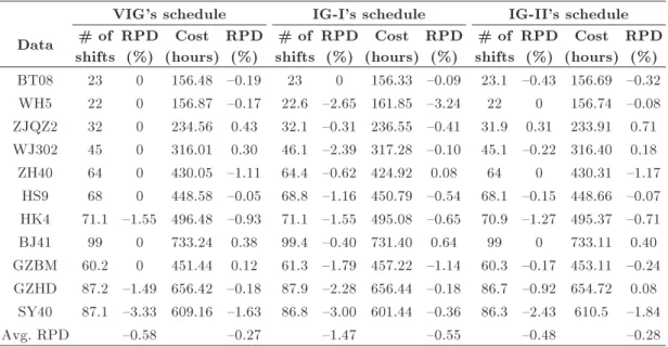
Table 4. Comparative average results of 10 runs for the GRAVIG and VIG and iterated greedy. VIG's schedule IG-I's schedule IG-II's schedule Data # of
shifts RPD
(%)
Cost (hours)
RPD (%)
# of shifts
RPD (%)
Cost (hours)
RPD (%)
# of shifts
RPD (%)
Cost (hours)
RPD (%) BT08 23 0 156.48 {0.19 23 0 156.33 {0.09 23.1 {0.43 156.69 {0.32 WH5 22 0 156.87 {0.17 22.6 {2.65 161.85 {3.24 22 0 156.74 {0.08 ZJQZ2 32 0 234.56 0.43 32.1 {0.31 236.55 {0.41 31.9 0.31 233.91 0.71 WJ302 45 0 316.01 0.30 46.1 {2.39 317.28 {0.10 45.1 {0.22 316.40 0.18 ZH40 64 0 430.05 {1.11 64.4 {0.62 424.92 0.08 64 0 430.31 {1.17
HS9 68 0 448.58 {0.05 68.8 {1.16 450.79 {0.54 68.1 {0.15 448.66 {0.07 HK4 71.1 {1.55 496.48 {0.93 71.1 {1.55 495.08 {0.65 70.9 {1.27 495.37 {0.71 BJ41 99 0 733.24 0.38 99.4 {0.40 731.40 0.64 99 0 733.11 0.40 GZBM 60.2 0 451.44 0.12 61.3 {1.79 457.22 {1.14 60.3 {0.17 453.11 {0.24 GZHD 87.2 {1.49 656.42 {0.18 87.9 {2.28 656.44 {0.18 86.7 {0.92 654.72 0.08
SY40 87.1 {3.33 609.16 {1.63 86.8 {3.00 601.44 {0.36 86.3 {2.43 610.5 {1.84
Avg. RPD {0.58 {0.27 {1.47 {0.55 {0.48 {0.28
this section, the IG with two values of d (i.e., dmin
and dmax used in the GRAVIG) are tested, denoted by
IG-I and IG-II, respectively. Their other ingredients are same as those in the GRAVIG. Average results of 10 independent runs of the IG-I and IG-II and specic comparative results with the GRAVIG are both illustrated in Table 4, where the RPD columns denote the GRAVIG's RPD over the IG-I and IG-II in terms of shift number and shift cost, respectively.
From Table 4, it can be seen that the GRAVIG performs better than both the IG-I and IG-II. The average RPDs over the IG-I and IG-II are {1.47% and {0.48%, respectively, in terms of shift number, and { 0.55% and {0.28%, respectively, in terms of shift cost. Furthermore, in terms of shift number, the GRAVIG is
no worse than the IG-I for all the 11 instances, while it performs better for 10 instances. Meanwhile, the GRAVIG is no worse than the IG-II for 10 instances, while it performs better for 7 instances.
5.5. Experiment on the solution distribution of the GRAVIG
We now turn our attention to testing the solution distribution of the GRAVIG. Average results of 20 independent runs of the GRAVIG are listed in Table 5. Table 5 shows that the shift numbers found in the 20 runs by the GRAVIG are the same for 6 instances, and only vary in 1 shift for 3 out of the remaining 5 instances. Moreover, there is no remarkable variation
Table 5. Results of 20 independent runs for the GRAVIG.
# of shifts Cost (hours)
Data Ave. Min. Max. Max.-Min. Ave. Min. Max. Std. dev.
BT08 23 23 23 0 156.13 155.58 158.83 0.72
WH5 22 22 22 0 156.76 154.93 159.18 1.32
ZJQZ2 31.9 31 32 1 234.99 232.35 238.10 1.77
WJ302 45.1 45 46 1 316.74 312.12 319.93 1.78
ZH40 64 64 64 0 426.33 419.98 432.85 3.20
HS9 68 68 68 0 448.68 447.92 448.75 0.20
HK4 70 70 70 0 492.28 486.62 496.23 2.01
BJ41 99 99 99 0 735.03 724.82 740.70 4.01
GZBM 60.05 60 61 1 450.85 447.80 454.12 1.80
GZHD 86.2 85 87 2 655.02 651.07 660.03 2.41
SY40 84.65 84 86 2 600.80 596.62 605.10 2.32
Avg. RPDa. 1.24% 0.75% 1.83%
between the 20 runs in terms of shift cost. This indicates that the GRAVIG is quite robust.
Furthermore, we also compare the results of the GRAVIG with the lower bound of the number of shifts illustrated in Section 4.1, the average RPD of the optimal schedules presented in Table 5 over the lower bound is 0.75% in terms of shift number. This demonstrates that the GRAVIG can obtain high-quality results.
6. Conclusions
This paper proposes a new approach for the public transit crew scheduling problem, named GRAVIG, which integrates GRA into a VIG algorithm. The GRA serves as a solver for shift selection during the schedule construction and destruction processes, which can be considered as an MADM problem. Moreover, in the GRAVIG, an elaborate biased probability destruction strategy is designed to maintain the `good' shifts in the schedule without losing randomness. Experiments on real-world instances show that the GRAVIG obtains high-quality schedules, which are close to the lower bounds obtained by the CPLEX in terms of shift number, and outperforms the AECS, VIG, and IG. Although we have presented this work in terms of public transport crew scheduling, it is suggested that the main idea of the GRAVIG can be extended to other problems.
Acknowledgement
The authors would like to thank the anonymous review-ers for their valuable comments and helpful recommen-dations. The work was supported by National Natural Science Foundation of China (Grants No. 71571076 and 71171087) and the Major Program of National Social Science Foundation of China (Grant No. 13&ZD175).
References
1. Shen, Y.D., Xu, J., and Zeng, Z.Y. \Public transit planning and scheduling based on AVL data in China", Int. T. Oper. Res., 23(6), pp. 1089-1111 (2016).
2. Kwan, R.S.K. and Kwan, A. \Eective search space control for large and/or complex driver scheduling problems", Ann. Oper. Res., 155(1), pp. 417-435 (2007).
3. Toth, A. and Kresz, M. \An ecient solution approach for real-world driver scheduling problems in urban bus transportation", Cent. Eur. J. Oper. Res., 21, pp. 75-94 (2013).
4. Shen, Y.D., Li, J.P., and Peng, K.K. \An estimation of distribution algorithm for public transport driver scheduling", Int. J. Operational Research, 28(2), pp. 245-262 (2017)
5. Kwan, R.S.K. \Case studies of successful train crew scheduling optimisation", J. Scheduling., 14(5), pp. 423-434 (2011).
6. Hickman, M., Mirchandani, P., Vo, S. (Eds.), Lecture Notes in Economics and Mathematical Systems, 600 (2008).
7. Lourenco, H.R., Paix~ao, J.P., and Portugal, R. \Multi-objective metaheuristics for the bus driver scheduling problem", Transport. Sci., 35(3), pp. 331-343 (2001).
8. Dias, T.G., de Sousa, J.P., and Cunha, J.F. \Genetic algorithms for the bus driver scheduling problem: a case study", J. Oper. Res. Soc., 53(3), pp. 324-335 (2002).
9. Li, J.P. and Kwan, R.S.K. \A fuzzy genetic algorithm for driver scheduling", Eur. J. Oper. Res., 147(2), pp. 334-344 (2003).
10. Park, T. and Ryu, K.R. \Crew pairing optimization by a genetic algorithm with unexpressed genes", J. Intell. Manuf., 17(4), pp. 375-383 (2006).
11. Shen, Y.D., Peng, K.K., Chen, K., and Li, J.P. \Evolu-tionary crew scheduling with adaptive chromosomes", Transport. Res. B-Meth., 56, pp. 174-185 (2013).
12. Cavique, L., Rego, C., and Themido, I. \Subgraph ejection chains and tabu search for the crew scheduling problem", J. Oper. Res. Soc., 50(6) pp. 608-616 (1999).
13. Shen, Y.D. and Kwan, R.S.K. \Tabu search for driver scheduling", Lecture Notes in Economics and Mathe-matical Systems, 505, pp. 121-135 (2001).
14. Yaghini, M., Karimi, M., and Rahbar, M. \A set cover-ing approach for multi-depot train driver schedulcover-ing", J. Comb. Optim., 29(3), pp. 636-654 (2015).
15. De Leone, R., Festa, P., and Marchitto, E. \Solving a bus driver scheduling problem with randomized multistart heuristics", Int. T. Oper. Res., 18(6), pp. 707-727 (2011).
16. Hana, R. and Kozan, E. \A hybrid constructive heuristic and simulated annealing for railway crew scheduling", Comput. Ind. Eng., 70, pp. 11-19 (2014).
17. Li, J.P., and Kwan, R.S.K. \A self-adjusting algorithm for driver scheduling", J. Heuristics., 11(4), pp. 351-367 (2005).
18. De Leone, R., Festa, P., and Marchitto, E. \A bus driver scheduling problem: a new mathematical model and a GRASP approximate solution", J. Heuristics., 17(4), pp. 441-466 (2011).
19. Aickelin, U., Burke, E.K., and Li, J.P. \An evolution-ary squeaky wheel optimization approach to personnel scheduling", IEEE. T. Evolut. Comput., 13(2), pp. 433-443 (2009).
20. Huang, S., Yang, T., and Wang, R. \Ant colony optimization for railway driver crew scheduling: from modeling to implementation", J. of the Chinese Insti-tute of Industrial Engineers, 28(6), pp. 437-449 (2011).
21. Li, J.P. \Fuzzy evolutionary approaches for bus and rail driver scheduling", Ph.D. Thesis, University of Leeds, England (2002).
22. Peng, K.K. and Shen, Y.D. \An evolutionary al-gorithm based on grey relational analysis for crew scheduling", J. Grey. Syst-UK., 28(3), pp. 75-88 (2016).
23. Framinan, J.M. and Leisten, R. \Total tardiness mini-mization in permutation ow shops: a simple approach based on a variable greedy algorithm", Int. J. Prod. Res., 46(22), pp. 6479-6498 (2008).
24. Tasgetiren, M.F., Pan, Q.K., Suganthan, P.N., and Buyukdagli, O. \A variable iterated greedy algorithm with dierential evolution for the no-idle permutation owshop scheduling problem", Comput. Oper. Res., 40(7), pp. 1729-1743 (2013).
25. Karabulut, K. and Tasgetiren, M.F. \A variable it-erated greedy algorithm for the traveling salesman problem with time windows", Inform. Sciences., 279, pp. 383-395 (2014).
26. Yin, M.S. \Fifteen years of grey system theory re-search: A historical review and bibliometric analysis", Expert. Syst. Appl., 40(7), pp. 2767-2775 (2013).
27. Rajesh, R. and Ravi, V. \Supplier selection in resilient supply chains: a grey relational analysis approach", J. Clean. Prod., 86, pp. 343-359 (2015).
28. Wu, L.F., Liu, S.F., Yao, L.G., and Yu, L. \Fractional order grey relational analysis and its application", Sci. Iran., 22(3), pp. 1171-1178 (2015).
29. Kuo, Y., Yang, T., and Huang, G.W. \The use of grey relational analysis in solving multiple attribute decision-making problems", Comput. Ind. Eng., 55, pp. 80-93 (2008).
30. Wang, P., Meng, P., Zhai, J.Y., and Zhu, Z.Q. \A hybrid method using experiment design and grey
relational analysis for multiple criteria decision making problems", Knowledge-Based Syst., 53, pp. 100-107 (2013).
31. Ding, J., Song, S., Gupta, J.N.D., Zhang, R., Chiong, R., and Wu, C. \An improved iterated greedy algo-rithm with a tabu-based reconstruction strategy for the no-wait owshop scheduling problem", Appl. Soft. Comput., 30, pp. 604-613 (2015).
32. Pranzo, M. and Pacciarelli, D. \An iterated greedy metaheuristic for the blocking job shop scheduling problem", J. Heuristics, 22, pp. 587-611 (2016).
Biographies
Kunkun Peng received his MS degree from Wuhan University of Technology, Wuhan, China, in 2010, and PhD degree from Huazhong University of Science and Technology, Wuhan, China, in 2016. His research inter-ests include optimization in public transport systems and crew scheduling.
Yindong Shen holds a PhD in Operations Research & Articial Intelligence from University of Leeds, UK. She is now a Professor at Huazhong University of Science and Technology, Wuhan, China. She is also a committee member of International Federation of Operational Research Societies-Developing Coun-tries Committee (IFORS-DCC), member of the stand-ing council of Operations Research Society of China (ORSC), and vice-presiding ocer of Operations Re-search Society of Hubei Province (ORSHB). Her major research interests are in modeling and applications of operations research, optimization in public transport systems, transit planning, vehicle and crew scheduling, and metaheuristics.