Intro-to-MATLAB

(1)

an interactive introduction to

MATLAB

(2)

(3)

A B O U T T H E C O U R S E

This course was developed in the School of Engineering to provide appropriate material for teaching MATLAB∗ in all engineering disciplines as well as to a wider audience. It is a self-study, self-paced course that emphasises responsible learning. Course material consists of this document used in conjunction with extensive online content. If you are a second-year engineering undergraduate student, there are also scheduled laboratory sessions where you can practice exercises and ask questions.

Who should use this document?

This document is targeted at those with no prior knowledge of MATLAB, and no previous programming experience. The aim, upon completion of the course, is to be competent using the most common features inMATLAB and be able to apply them to solve engineering problems.

What is in this document?

This document forms part of a self-study course to help you get started with MATLAB. It should be used along with the support-ing online materials available at the course website

(http://www.eng.ed.ac.uk/teaching/courses/matlab). The main body of this document contains the fundamental topics for the course and there are also several more advanced topics given in appendices. How to use this document?

This document contains different elements designed to make your learning experience as smooth as possible. To benefit the most from these elements you are encouraged to use the online PDF version

of this document. One of the first things you’ll notice is that this You can use the commenting tools in Adobe Reader to add your own notes to this PDF document document contains many links: those inredindicate a link to online

material, and those inblueindicate a link to another section of this document.

A key part of this course are the screencasts, which are video screen captures(http://en.wikipedia.org/wiki/Screencast). In this ∗ MATLAB® is a registered trademark of MathWorks

(4)

Figure 1: A University of Edinburgh screencast

document screencasts are indicated by a link in a blue box with a clapperboard icon, like the example shown.

Watching the screencasts and trying the examples for yourself will help you develop your skills in MATLABmore quickly!

Getting started

(http://www.eng.ed.ac.uk/teaching/courses/matlab/getting-started.shtml) Clicking on a link to a screencast will take you to the appropriate page on the course website where you will see the opening image to a University of Edinburgh screencast presented in the video player (Figure 1). Watching and learning from the screencasts are an essential part of the course and will help you develop your skills inMATLAB more quickly.

You will also notice two other types of blue box environments in this document: one is for Hints and Tips (with a question mark icon), and the other contains exercises that you should complete (with an inkwell icon).

Hints and Tips

Throughout this document you will also seeHints and Tipsboxes like this one. Please read these as they contain useful hints!

(5)

An example exercise Example exercise solutions

Additionally there are grey box environments in this document. Like the example shown (Listing1), these contain code listings that demonstrate actual MATLAB code. Line numbers are given to the left of the listings to make is simpler to refer to specific bits of code. Very often you will be required to copy and paste the listing intoMATLABand try running it for yourself.

Listing 1: Example of a code listing 1 >> 5+5

2 ans =

3 10

Sources of help and further reading

There are a huge number of textbooks published on the subject of MATLAB! A user-friendly textbook that provides a good

intro-duction toMATLABis: Available fromAmazon

for c.£15 • Gilat, A. (2008).MATLAB: An Introduction With

Applica-tions. John Wiley & Sons, Inc., 3rd edition.

There are a couple of further textbooks listed in theBibliography section at the end of this document. However, throughout this course and beyond, the most important source of help is the docu-mentation built-in toMATLAB. It is easily searchable, and because MATLABcontains many built-in functions it is worth checking out before starting to write your own code.

• MATLABhelp documentation

(http://www.mathworks.com/access/helpdesk/help/techdoc/) Accessed through the help menu inMATLAB, or online. • MATLAB Central

(http://www.mathworks.co.uk/matlabcentral/)

An open exchange for users, with code snippets, help forums and blogs. A great place to search for specific help!

(6)

Development of the course

The development of this course was funded through The Edinburgh Fund Small Project Grant which is part of The University of Edin-burgh Campaign

(http://www.edinburghcampaign.com/alumni-giving/grants). The material for this course was developed by Dr. Tina Düren, Dr. Antonis Giannopoulos, Dr. Guillermo Rein, Dr. John Thompson, and Dr. Craig Warren.

(7)

C O N T E N T S

0.1 What isMATLAB? . . . 1

0.2 How isMATLAB used in industry? . . . 1

1 basic concepts 3 1.1 MATLAB in the School of Engineering . . . 3

1.2 TheMATLAB environment . . . 3

1.3 Basic calculations . . . 4

1.4 Variables and arrays . . . 7

1.5 Solving systems of linear equations . . . 13

2 plotting 19 2.1 Simple 2dplotting . . . 19

2.1.1 Multiple plots in one Figure Window . . . 23

2.2 Curve-fitting . . . 25

2.3 3d plotting using plot3 and surf . . . 26

3 scripts and functions 33 3.1 Script files . . . 33

3.2 Functions . . . 39

4 decision making 45 4.1 Relational and logical operations . . . 45

4.2 The if-else statement . . . 48

5 loops 57 5.1 for loops . . . 57

5.2 while loops . . . 60

a advanced topic: the switch statement 67 b advanced topic: vectorisation 69 c additional exercises 71 c.1 Basic Concepts . . . 71

c.2 Plotting . . . 76

c.3 Scripts and Functions . . . 83

c.4 Decision Making . . . 89

c.5 Loops . . . 90

bibliography 93

(8)

L I S T O F S C R E E N C A S T S

TheMATLAB desktop . . . 4

Exercise 1 Solutions . . . 6

Variables and simple arrays . . . 9

The dot operator . . . 10

Indexing arrays . . . 12

Creating a simple plot . . . 21

Plotting experimental data . . . 22

Basic Curve-fitting . . . 25

Creating a simple script . . . 35

Creating a function . . . 42

The if-else statement . . . 51

The for loop . . . 59

The while loop . . . 62

(9)

L I S T O F E X E RC I S E S

Exercise 1: Basic calculations . . . 6

Exercise 2: Variables and arrays . . . 15

Exercise 3: Simple 2d plotting . . . 24

Exercise 4: 3_d plotting . . . 30

Exercise 5: Scripts . . . 37

Exercise 6: Functions . . . 43

Exercise 7: Decision making . . . 54

Exercise 8: Loops . . . 65

(10)

L I S T O F TA B L E S

Table 1 Arithmetic operations . . . 6

Table 2 Element-by-element arithmetic operations . . . 10

Table 3 Line styles in plots . . . 20

Table 4 Colours in plots . . . 21

Table 5 Function definitions, filenames, input and output variables 40 Table 6 Relational operators . . . 45

Table 7 Logical operators . . . 45

Table 8 Friction experiment results . . . 73

Table 9 Results of a tension test on an aluminium specimen . . 76

Table 10 Coefficients for the cubic equation for the heat capacity of gases . . . 85

(11)

A B O U T M AT L A B

0.1 what is matlab?

MATLABis produced by MathWorks, and is one of a number of commercially available software packages for numerical computing and programming. MAT-LAB provides an interactive environment for algorithm development, data visualisation, data analysis, and numerical computation. MATLAB, which derives its name from MATrix LABoratory, excels at matrix operations and graphics. Its main competitors are Maple, Mathematica, and Mathcad, each

with their own strengths and weaknesses. MATLABR2011a

student version is available for around £50

MATLAB is available in both commercial and academic versions with new releases binannually e. g. R2011a (released around March 2011), and R2011b (released around September 2011).MATLAB itself is the core product and is augmented by additional toolboxes, many of which have to be purchased separ-ately. If you want to run MATLABon your own computer MathWorks offers a student version (http://www.mathworks.com/academia/student_version/) with some of the most commonly used toolboxes for around £50. The accom-panying online material, and the screenshots in this document are based on MATLABR2009a running under Microsoft Windows XP.

0.2 how is matlab used in industry?

Knowing how to use MATLABis a vital skill for many engineering jobs! The ability to use tools such asMATLAB is increasingly required by

employ-ers of graduate engineemploy-ers in industry. Many job adverts specifically mention knowledge of MATLABas an essential skill.

MATLAB is a widely-used tool in many different fields of engineering and science. The following is a brief list of examples from Chemical, Civil, Electrical, and Mechanical Engineering:

• Motorsport Teams Improve Vehicle Performance with MathWorks Tools

(http://www.mathworks.com/products/simmechanics/userstories.html?file=11197) • Bell Helicopter Develops the First Civilian Tiltrotor

(http://www.mathworks.com/company/newsletters/news_notes/oct06/bellhelicopter.html)

(12)

2 List of Tables

• Greenhouse Designed with MATLAB and Simulink Revolutionizes Agri-culture in Arid Coastal Regions

(http://www.mathworks.com/company/user_stories/userstory2347.html?by=industry) • Thames Water Aims to Reduce Leaks by More Than 25% Using a

MATLAB-Based Leak-Location System

(http://www.mathworks.com/company/user_stories/userstory2354.html?by=industry) • Samsung UK Develops 4G Wireless Systems with Simulink

(http://www.mathworks.com/company/user_stories/userstory10725.html?by=industry) • Cambridge Consultants Develops WiMAX Test Bench for Aspex

Semi-conductor with MATLAB

(http://www.mathworks.com/company/user_stories/userstory10996.html?by=industry) • Halliburton Makes Oil Exploration Safer Using MATLAB and Neural

Networks

(http://www.mathworks.com/industrial-automation-machinery/userstories.html? file=2355&title=Halliburton%20Makes%20Oil%20Exploration%20Safer%20Using%20 MATLAB%20and%20Neural%20Networks)

(13)

1

B A S I C C O N C E P T S

1.1 matlab in the school of engineering

MATLABis currently available under Microsoft Windows 7 and Linux oper-ating systems in the School of Engineering Computing Labs

(http://www.eng.ed.ac.uk/it/TLabs/), and also under Microsoft Windows 7 in

all Open Access Computing Labs ( http://www.ed.ac.uk/schools-departments/information-services/services/computing/desktop-personal/open-access/locations/locations).

To launchMATLAB under Microsoft Windows 7 in a University of Edin-burgh computing lab click on its shortcut, located at Start →All Programs

→MATLAB →MATLAB R2011a.

1.2 the matlab environment

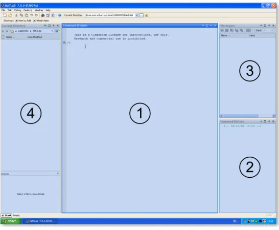
When you launch MATLAByou are presented with theMATLABdesktop (Figure2) which, by default, is divided into 4 windows:

1. Command Window: This is the main window, and contains the command prompt (»). This is where you will type all commands.

2. Command History: Displays a list of previously typed commands. The command history persists across multiple sessions and commands can be dragged into the Command Window and edited, or double-clicked to run them again.

3. Workspace: Lists all the variables you have generated in the current session. It shows the type and size of variables, and can be used to quickly plot, or inspect the values of variables.

4. Current Directory: Shows the files and folders in the current directory. The path to the current directory is listed near the top of theMATLAB desktop. By default, aMATLABfolder is created in your home directory on your M:drive, and this is where you should save your work.

You will use and become more familiar with the different areas of theMATLAB desktop as you progress through this course.

(14)

4 basic concepts

1

4

3

2

Figure 2: The MATLABdesktop The _MATLAB desktop

(http://www.eng.ed.ac.uk/teaching/courses/matlab/unit01/MATLAB-desktop.shtml)

Remember you can pause the screencasts at any time and try the

examples for yourself. 1.3 basic calculations

MATLAB can perform basic calculations such as those you are used to doing on your calculator. Listings 1.1–1.5 gives some simple examples (and results) of arithmetic operations, exponentials and logarithms, trigonometric functions, and complex numbers that can be entered in the Command Window.

Listing 1.1: Addition 1 >> 4+3

2 ans =

3 7

Try using_MATLAB as an expensive

calculator! Listing 1.2: Exponentiation 1 >> 2^2

2 ans =

(15)

1.3 basic calculations 5

Listing 1.3: Trigonometry 1 >> sin(2*pi)+exp(−3/2)

2 ans =

3 0.2231

The arguments to trigonometric functions should be given in radians.

Comments:

• MATLABhas pre-defined constants e. g. π may be typed aspi. • You must explicitly type all arithmetic operations e. g.sin(2*pi)not

sin(2pi).

• sin(x)and exp(x)correspond to sin(x) andex respectively.

Listing 1.4: Complex numbers 1 >> 5+5j

2 ans =

3 5.0000 + 5.0000i

Comments:

• Complex numbers can be entered using the basic imaginary unit iorj. Listing 1.5: More trigonometry

1 >> atan(5/5) 2 ans =

3 0.7854

5 _{>> 10*log10(0.5)} 6 ans =

7 −3.0103

Comments:

• atan(x)and log10(x)correspond to tan−1(x) and log10(x)

respect-ively.

Built-in functions

There are many other built-inMATLAB functions for performing basic cal-culations. These can be searched from the Help Browser which is opened by clicking on its icon (like the icon used to indicate this Hints and Tips section) in the MATLABdesktop toolbar.

(16)

6 basic concepts

Table 1: Arithmetic operations command description

+ Addition

− Subtraction

* Multiplication

/ Division

^ Exponentiation

Exercise 1: Basic calculations

1. Launch MATLAB and explore the different areas of the MATLAB desktop.

2. Try the basic calculations given in Listings1.1–1.5, and check you get the correct answers.

3. Arithmetic operations Compute the following:

• 25

25₋₁ and compare with 1− 1 25

−1

• √5−1

(√5+1)2

[Answers: 1.0323, 1.0323, 0.1180] 4. Exponentials and logarithms

Compute the following: • e3

• ln(e3) • log₁₀(e3) • log10(105)

[Answers: 20.0855, 3, 1.3029, 5] 5. Trigonometric operations

Compute the following: • sin(π₆)

• cos(π) • tan(π₂)

• sin2(π₆) +cos2(π₆)

[Answers: 0.5, -1, 1.6331E16, 1] Exercise 1 Solutions

(http://www.eng.ed.ac.uk/teaching/courses/matlab/unit01/Ex1-Solutions.shtml)

(17)

1.4 variables and arrays 7 You may have noticed that the result of each of the basic calculations you performed was always assigned to a variable calledans. Variables are a very important concept inMATLAB.

1.4 variables and arrays

A variable is a symbolic name associated with a value. The current value of the variable is the data actually stored in the variable. Variables are very important inMATLAB because they allow us to easily reference complex and changing data. Variables can reference different data types i. e. scalars, vectors, arrays, matrices, strings etc.... Variable names must consist of a letter which can be followed by any number of letters, digits, or underscores. MATLABis case sensitive i. e. it distinguishes between uppercase and lowercase letters e. g.A and aare not the same variable.

Variables you have created in the current MATLABsession can be viewed in a couple of different ways. The Workspace (shown in Figure2) lists all the current variables and allows you to easily inspect their type and size, as well as quickly plot them. Alternatively, the whoscommand can be typed in the Command Window and provides information about the type and size of current variables. Listing 1.6 shows the output of thewhos command after storing and manipulating a few variables.

Listing 1.6: Using thewhoscommand 1 >> a = 2

2 a =

3 2

4 >> b = 3

5 b =

6 3

7 _{>> c = a*b} 8 c =

9 6

10 >> edinburgh = a+5

11 edinburgh =

12 7

13 >> whos

14 Name Size Bytes Class Attributes

16 a 1x1 8 double

17 b 1x1 8 double

18 c 1x1 8 double

19 edinburgh 1x1 8 double

Arrays are lists of numbers or expressions arranged in horizontal rows and vertical columns. A single row, or single column array is called a vector. An

(18)

8 basic concepts

array withmrows and ncolumns is called a matrix of sizem×n. Listings1.7–

1.10 demonstrate how to create row and column vectors, and matrices in MATLAB.

Listing 1.7: Creating a row vector 1 >> x = [1 2 3]

2 x =

3 1 2 3

• Square brackets are used to denote a vector or matrix. • Spaces are used to denote columns.

Listing 1.8: Creating a column vector 1 >> y = [4; 5; 6]

2 y =

3 4

4 5

5 6

• The semicolon operator is used to separate columns. Listing 1.9: The transpose operator 1 >> x'

2 ans =

3 1

4 2

5 3

7 >> y'

8 ans =

9 4 5 6

• The single quotation mark'transposes arrays, i.e. the rows and columns are interchanged so that the first column becomes the first row etc... A more efficient method for entering vectors, especially those that con-tain many values, is to use ranges. Instead of entering each individual value separately, a range of values can be defined as shown in Listing 1.10.

(19)

1.4 variables and arrays 9

Listing 1.10: Creating vectors using ranges 1 >> z = 8:1:10

2 z =

3 8 9 10

5 >> v = linspace(0,10,5)

6 v =

7 0 2.5000 5.0000 7.5000 10.0000

Comments:

• A range can be created using the colon operator, e. g. 8:1:10 means create a range that starts at 8 and goes up in steps of size 1 until 10. • A range can also be created using the linspacefunction,

e. g.linspace(0,10,5) means create a range between 0 and 10 with 5 linearly spaced elements.

clear and clccommands

Theclearcommand can be used if you want to clear the current workspace of all variables. Additionally, theclccommand can be used to clear the Command Window, i.e. remove all text.

Variables and simple arrays

(http://www.eng.ed.ac.uk/teaching/courses/matlab/unit01/variables-arrays.shtml)

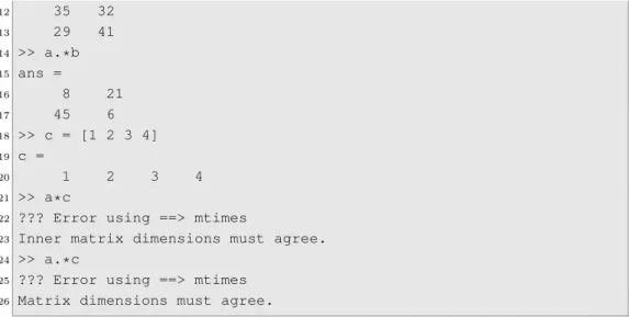
MATLAB excels at matrix operations, and consequently the arithmetic operators such as multiplication (*), division (/), and exponentiation (^) perform matrix multiplication, division, and exponentiation, when used on a vector, by default. To perform an element-by-element multiplication, division, or exponentiation you must precede the operator with a dot. Table 2 and Listing 1.11demonstrate the dot operator.

Listing 1.11: The dot operator 1 >> clear

2 >> a = [2 3; 5 1]

3 a =

4 2 3

5 5 1

6 >> b = [4 7; 9 6]

7 b =

8 4 7

9 9 6

10 _{>> a*b} 11 ans =

(20)

10 basic concepts

12 35 32

13 29 41

14 _{>> a.*b} 15 ans =

16 8 21

17 45 6

18 >> c = [1 2 3 4] 19 c =

20 1 2 3 4

21 _{>> a*c}

22 ??? Error using ==> mtimes

23 Inner matrix dimensions must agree.

24 _{>> a.*c}

25 ??? Error using ==> mtimes

26 Matrix dimensions must agree.

Comments:

• The dot operator signifies an element-by-element operation. The dot can be used for multiplication .*, division./, or exponentiation .^ of elements of vectors that are the same size. Omitting the dot before an arithmetic operator meansMATLAB performs the matrix version of the operation.

• On Line 21 we tried to perform a matrix multiplication of a 2×2 matrix with a 1×4 matrix. This results in an error because you can only multiply two matrices if the number of columns in the first equals the number of rows in the second.

• On Line 24 we get a similar error if we try to perform an element-by-element multiplication, as this does not make any sense for matrices of different sizes.

Table 2: Element-by-element arithmetic operations command description

.* Element-by-element multiplication ./ Element-by-element division .^ Element-by-element exponentiation

The dot operator

(http://www.eng.ed.ac.uk/teaching/courses/matlab/unit01/dot-operator.shtml)

(21)

1.4 variables and arrays 11

Read _MATLAB error messages! ??? Error using ==> mtimes

Inner matrix dimensions must agree.

This error message example usually indicates you tried to perform a matrix operation when you intended an element-by-element operation. You should check your code for a missing dot operator.

You can access individual elements, entire rows and columns, and subsets of matrices using the notationmatrix_name(row,column). Listing1.12

demon-strates how to access elements in a matrix. Square brackets[ ]

are used when creating vectors, arrays and matrices, and round brackets( )when accessing elements in them.

Listing 1.12: Accessing elements of matrices 1 >> w = [1 2 3 4; 5 6 7 8; 9 10 11 12]

2 w =

3 1 2 3 4

4 5 6 7 8

5 9 10 11 12

7 >> size(w)

8 ans =

9 3 4

11 >> w(1,1)

12 ans =

13 1

15 >> w(3,1)

16 ans =

17 9

19 >> w(3,:)

20 ans =

21 9 10 11 12

23 >> w(2,4) = 13

24 w =

25 1 2 3 4

26 5 6 7 13

27 9 10 11 12

29 >> v = w(1:2,2:3) 30 v =

31 2 3

32 6 7

34 >> z = w([2,3],[2,4])

35 z =

36 6 13

(22)

12 basic concepts

Comments:

• On Line 7 the sizecommand returns the number of rows and columns in the matrix.

• On Lines 11, 15 and 19, when accessing an individual element in a matrix, the first number after the round bracket refers to the row number (row index), and second number refers to the column number (column index). • On Line 19 the colon operator is used to denote all of the columns, i.e. all the columns in the third row are selected. The colon operator can also be used as a row index to denote all rows.

• Line 23 demonstrates accessing a single element in the matrixwto change its value.

• On Line 29 a new matrixv is created as a sub-matrix ofw.

• Finally, on Line 34 a new matrixzis created as a sub-matrix ofw. Square brackets are used within the round brackets to enclose the list of row and column numbers.

Indexing arrays

(http://www.eng.ed.ac.uk/teaching/courses/matlab/unit01/indexing-arrays.shtml)

Self Test Exercise: Indexing arrays 1. †_{The following matrix is defined:}

M=        

6 9 12 15 18 21

4 4 4 4 4 4

2 1 0 −1 −2 −3

−6 −4 −2 0 2 4

       

Evaluate the following expressions without using MATLAB. Check your answers withMATLAB.

a) A = M([1,3], [2,4]) b) B = M(:, [1,4:6]) c) C = M([2,3], :)

† Question adapted from Gilat, A. (2008)._MATLAB: An Introduction With Applications. John Wiley & Sons, Inc., 3rd edition. Copyright ©2008 John Wiley & Sons, Inc. and reprinted with permission of John Wiley & Sons, Inc.

(23)

1.5 solving systems of linear equations 13

1.5 solving systems of linear equations

Solving systems of linear equations is one of the most common computations in science and engineering, and is easily handled by MATLAB. Consider the following set of linear equations.

5x=3y−2z+10 8y+4z=3x+20 2x+4y−9z=9

This set of equations can be re-arranged so that all the unknown quantities are on the left-hand side and the known quantities are on the right-hand side.

5x−3y+2z=10

−3x+8y+4z=20 2x+4y−9z=9

This is now of the form AX=B, whereAis a matrix of the coefficients of the

unknowns, A=     

5 −3 2

−3 8 4

2 4 −9

    

xis the vector of unknowns,

X=      x y z     

and Bis a vector containing the constants.

B=      10 20 9     

Listing 1.13shows the code used to solve the system of linear equations in MATLAB. The rules of matrix algebra apply i.e. the result of multiplying a

(24)

14 basic concepts

Listing 1.13: Solving a system of linear equations 1 >> A = [5 −3 2; −3 8 4; 2 4 −9];

2 >> B = [10; 20; 9;]; 3 >> X = A\B

4 X =

5 3.4442

6 3.1982

7 1.1868

Using a semi-colon at the end of a command prevents the results being displayed in the Command Window.

Comments:

• On Line 1 the matrix, A, of coefficients of the unknowns is entered.

• On Line 2 the vector, B, containing the constants is entered.

• On Line 3 the vector,X, containing the unknowns, is calculated by using

the matrix left divide operator to divideA byB.

Listing1.14demonstrates how to check the solution obtained in Listing1.13. Listing 1.14: Checking the solution of a system of linear equations

1 _{>> C = A*X} 2 C =

3 10.0000

4 20.0000

5 9.0000

Not all systems of linear equations have a unique solution. If there are fewer equations than variables, the problem is under-specified. If there are more equations than variables, it is over-specified.

The left division or backslash operator (\)

In MATLAB the left division or backslash operator (\) is used to solve equations of the formAX=B i.e. X = A\B. Gaussian elimination is used to perform this operation.

(25)

Exercise 2: Variables and arrays

1. Create the variables to represent the following matrices:

A= h

12 17 3 4

i B=     

5 8 3

1 2 3

2 4 6

     C=      22 17 4     

a) Assign to the variable x1 the value of the second column of matrix A.

b) Assign to the variablex2 the third column of matrixB. c) Assign to the variable x3 the third row of matrixB.

d) Assign to the variablex4 the first three values of matrix Aas the first row, and all the values in matrix B as the second, third and fourth rows.

2. If matrix A is defined using the MATLAB code

A = [1 3 2; 2 1 1; 3 2 3], which command will produce the following matrix? B=   3 2 2 1  

3. Create variables to represent the following matrices:

A=     

1 2 3

2 2 2

−1 2 1

     B=     

1 0 0

1 1 0

1 1 1

     C=      1 1 2 1 1 2     

a) Try performing the following operations: A+B,A*B,A+C,B*A,B−A, A*C, C−B, C*A. What are the results? What error messages are generated? Why?

b) What is the difference betweenA*Band A.*B?

4. Solve the following systems of linear equations. Remember to verify your solutions.

a)

−2x+y=3 x+y=10

(26)

16 basic concepts

Exercise 2: Variables and arrays (continued) 4. continued

b)

5x+3y−z=10 3x+2y+z=4 4x−y+3z=12

c)

x1−2x2−x3+3x4=10 2x₁+3x₂+x₄=8 x₁−4x₃−2x₄=3

−x₂+3x₃+x₄= −7

5. Create a vectort that ranges from 1 to 10 in steps of 1, and a vector thetathat ranges from 0 to πand contains 32 elements. Now compute

the following:

x=2sin(θ)

y= t−1

t+1 z= sin(θ

2₎ θ2

6. A discharge factor is a ratio which compares the mass flow rate at the end of a channel or nozzle to an ideal channel or nozzle. The discharge factor for flow through an open channel of parabolic cross-section is:

K= 1.2

x

p

16x2₊₁₊ 1 4xln

p

16x2₊₁₊_4x

−2₃

,

where x is the ratio of the maximum water depth to breadth of the

channel at the top of the water. Determine the discharge factors forxin

the range 0.45 to 0.90 in steps of 0.05. 7. Points on a circle

All points with coordinates x = rcos(θ) and y = rsin(θ), where r is

a constant, lie on a circle with radius r, i. e. they satisfy the equation x2+y2=r2. Create a column vector forθ with the values0,π/4,π/2, 3π/4,π, and 5π/4. Take r= 2 and compute the column vectorsxand y. Now check that x and y indeed satisfy the equation of a circle, by

(27)

Exercise 2: Variables and arrays (continued) 8. Geometric series

The sum of a geometric series1+r+r2+r3+. . .+rn approaches the

limit 1

1−r for r < 1asn→∞. Take r=0.5 and compute sums of series

0 to 10, 0 to 50, and 0 to 100. Calculate the aforementioned limit and compare with your summations. Do the summation using the built-in sum function.

Exercise 2 Solutions

Additional Exercises

(28)

(29)

2

P L O T T I N G

MATLAB is very powerful for producing both 2dand 3d plots. Plots can be created and manipulated interactively or by commands. MATLABoffers a number of different formats for exporting plots, including EPS (Encapsulated PostScript), PDF (Portable Document Format) and JPEG (Joint Photographic Experts Group), so you can easily include MATLABplots in your reports. 2.1 simple 2d plotting

The simplest and most commonly used plotting command isplot(x,y), where x andyare simply vectors containing the xandycoordinates of the data to

be plotted. Listing2.1 demonstrates the commands used to create a plot of the function, f(x) =e−10xsin(x), which is shown in Figure 3.

Listing 2.1: A simple plot 1 >> x = 0:0.1:20;

2 >> y = exp(−x/10).*sin(x);

3 >> plot(x,y), grid on, xlabel('x'), ...

4 ylabel('f(x) = e^{−x/10} sin(x)'), title('A simple plot')

Comments:

• The vectors containing the xand ydata must be the same length. • The plot command can be used to plot multiple sets of data on the same

axes, i. e.plot(x1,y1,x2,y2).

• The dot-dot-dot... (ellipsis) notation is used to indicate that Lines 3 and 4 are one long line. The ellipsis notation just allows the line to be broken to make it more readable. Each comma-separated command could also have been typed on a separate line.

When MATLABexecutes a plotting command, a new Figure Window opens with the plot in it. The following list gives the most common commands for changing plot properties.

• grid ondisplays the grid!

(30)

20 plotting

Figure 3: Plot off(x) =e−10x sin(x)

• xlabel('My x−axis label'),ylabel('My y−axis label'), andtitle('My title') can be used to label the corresponding parts of the plot. You must enclose

your labels with single quotes which denotes a string of text.

• legend('Data1','Data2') is used to place a legend and label the data-sets when you have multiple data-sets on one plot.

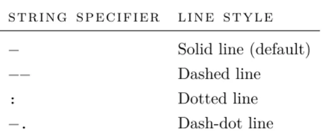
• You can specify line style and colour within the plot command e. g. plot(x1,y1,'b−',x2,y2,'r−−'). This command would make the first data-set a solid blue line, and the second data-set a dashed red line. Tables3–4 gives some of the most common line styles and colours.

Table 3: Line styles in plots string specifier line style

− Solid line (default)

−− Dashed line

: Dotted line

(31)

2.1 simple 2d plotting 21

Table 4: Colours in plots

string specifier line colour

r Red

g Green

b Blue (default)

w White

k Black

Plot properties can also be manipulated interactively (without having to issue commands) by clicking on theShow Plot Tools icon in the Figure Window toolbar, shown in Figure4. Properties such as the axis limits, gridlines, line style, colour and thickness, text font type and size, and legend etc... can all be adjusted be clicking on the appropriate parts of the plot.

Figure 4:Show Plot Toolstoolbar icon in Figure Window Producing good plots

Whether you manipulate your plots via commands or interactively, here is some useful advice for producing good plots in MATLAB.

• Give your plot an informative title

e. g. title('Stress vs. strain of steel')

• Label your axes and remember to include units where appropriate e. g. xlabel('Strain'), ylabel('Stress (MPa)')

• Use line colours and styles carefully so that multiple data-sets can be easily distinguished e. g.plot(x1,y1,'b−',x2,y2,'r−−'), grid on • Remember to insert a legend when you are plotting multiple data-sets

on one plot e. g.legend('Carbon steel','Stainless steel') Creating a simple plot

(http://www.eng.ed.ac.uk/teaching/courses/matlab/unit02/simple-plot.shtml)

(32)

22 plotting

MATLABhas many built-in plot types, and a great way of getting a quick overview of all the different plot types is to select a variable in your Workspace Browser, click on the disclosure triangle next to theplot toolbar icon and select More plots..., as shown in Figure5a. This will launch the Plot Catalog shown in Figure 5b.

(a) Accessing thePlot Catalog

(b) ThePlot Catalog

Figure 5:The Plot Catalog Plotting experimental data

(http://www.eng.ed.ac.uk/teaching/courses/matlab/unit02/plot-exp-data.shtml)

(33)

2.1 simple 2d plotting 23

Importing data from external sources

You can import data from other programs into MATLAB using the Copy →Paste method, or using the Import Data Wizard, found at File →Import Data..., for Microsoft Excel data, Comma-separated value files and more. There are also functions,xlsread and xlswrite.

2.1.1 Multiple plots in one Figure Window

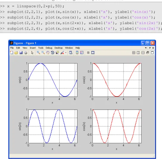
The subplotcommand can be used to display a number of different plots in a single Figure Window, as shown in Figure6. The subplotcommand takes three arguments that determine the number and location of plots in the Figure Window. For example,subplot(2,2,1)specifies that the Figure Window will be divided into 2 rows and 2 columns of plots, and selects the first subplot to plot into. Listing2.2 shows an example of usage of thesubplot command.

Listing 2.2: Using thesubplotcommand 1 _{>> x = linspace(0,2*pi,50);}

2 >> subplot(2,2,1), plot(x,sin(x)), xlabel('x'), ylabel('sin(x)'); 3 >> subplot(2,2,2), plot(x,cos(x)), xlabel('x'), ylabel('cos(x)');

4 _{>> subplot(2,2,3), plot(x,sin(2*x)), xlabel(}'x'), ylabel('sin(2x)');

5 _{>> subplot(2,2,4), plot(x,cos(2*x)), xlabel(}'x'), ylabel('cos(2x)');

(34)

24 plotting

Exercise 3: Simple 2d plotting

Please save all the plots you produce using theFile→Saveoption in the Figure Window. This should save a file with the MATLAB default Figure format which uses a.fig file extension.

1. Plot the following functions (you will need to decide on appropriate ranges forx):

• y= _x1, with a blue dashed line.

• y=sin(x)cos(x), with a red dotted line. • y=2x2₋_3x₊₁_{, with red cross markers.}

Turn the grid onin all your plots, and remember to label axes and use a title.

2. Given the following function:

s=acos(φ) + q

b2_{− (}_asin₍_φ_{) −}_c₎2

Plot s as a function of angle φ when a = 1, b = 1.5, c = 0.3, and 0₆φ₆360◦.

3. Plot the following parametric functions (you will need to use the axis equalcommand after yourplot command to forceMATLAB to make the x-axis and y-axis the same length):

a) A circle of radius 5 (revisit Ex2 Q7) b) Leminscate (−π/4₆φ₆π/4)

x=cos(φ)p2cos(2φ)

y=sin(φ)p2cos(2φ)

c) Logarithmic Spiral (0₆φ₆6π;k=0.1)

x=ekφcos(φ)

y=ekφsin(φ)

Exercise 3 Solutions

(35)

2.2 curve-fitting 25

2.2 curve-fitting

MATLABprovides a number of powerful options for fitting curves and adding trend-lines to data. The Basic Fitting Graphical User Interface (GUI) can be selected from Figure Windows by selecting Basic fitting from the Tools menu, and offers common curve-fitting options for 2d plots. More advanced functionality, including 3dfits, can be accessed from the Curve Fitting Toolbox using tools such ascftool(for curve fitting) andsftool(for surface fitting)∗.

Basic Curve-fitting

(http://www.eng.ed.ac.uk/teaching/courses/matlab/unit02/basic-curve-fitting.shtml)

An alternative to the Basic Fitting GUI are the functions polyfit and polyvalwhich can be used to do basic curve-fitting programmatically. List-ing 2.3 demonstrates how polyfit can be used to fit a polynomial to a data-set.

Listing 2.3: Syntax ofpolyfitcommand 1 coeff = polyfit(xdata,ydata,n);

Comments:

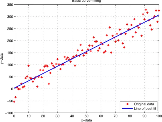
• coeffis a vector containing the coefficients for the polynomial of best fit, xdata andydataare vectors containing the independent and dependent variables, and ndenotes the degree of the polynomial to be fitted. After using polyfityou can use thepolyval function to evaluate the poly-nomial of best fit, given by the set of coefficientscoeff, at specific values of your data. This creates a vector of points of the fitted data,y_fit. Listing 2.4 and Figure7demonstrate the use of both thepolyfitandpolyvalfunctions. The data used for fitting can be downloaded (linear_fit_data.mat) and upon double-clicking the .mat file, the data will be loaded into _MATLAB and assigned to the variables x and y. This data is best fitted using a linear or straight-line fit.

Listing 2.4: Usingpolyfitandpolyvalfor curve-fitting 1 >> coeff = polyfit(x,y,1);

2 >> y_fit = polyval(coeff,x);

3 >> plot(x,y,'r+',x,y_fit), grid on, xlabel('x−data'), ...

4 ylabel('y−data'), title('Basic curve−fitting'), ...

5 legend('Original data','Line of best fit','Location','SouthEast')

(36)

26 plotting

0 10 20 30 40 50 60 70 80 90 100

ï100

ï50 0 50 100 150 200 250 300 350

xïdata

y

ï

data

Basic curveïfitting

Original data Line of best fit

Figure 7: Usingpolyfitandpolyvalfor curve-fitting Comments:

• 'r+'plots the xand ydata using red crosses.

• You can insert a legend from the Command Window using thelegend command, and specifying the text in the legend using strings.

2.3 3d plotting using plot3 and surf

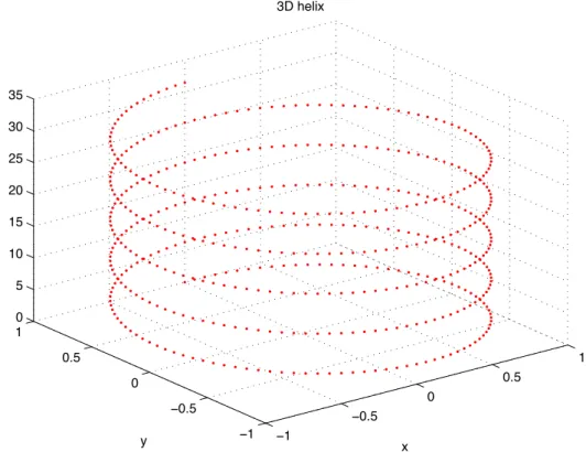
MATLAB is hugely powerful and versatile at visualising data in 3d. There are a number of built-in functions for producing different types of 3dplots e. g. points, lines, surfaces and volumes.

The 2dplot function becomesplot3(x,y,z) for plotting points and lines in 3d space. Listing 2.5 and Figure 8 demonstrate using plot3 to plot the points on a helix in 3dspace.

Listing 2.5: Using plot3to plot points on a helix 1 _{>> t = 0:pi/50:10*pi;}

2 >> plot3(sin(t),cos(t),t,'r.'), grid on, ...

(37)

2.3 3d plotting using plot3 and surf 27

ï1

ï0.5

0

0.5

1

ï1 ï0.5

0 0.5

1 0 5 10 15 20 25 30 35

x 3D helix

y

z

Figure 8: Usingplot3to plot points on a helix

For plotting surfaces and contours two commonly used functions aresurf(x,y,z) and mesh(x,y,z) where x,y, and z are coordinates of points on a surface. Before you use either of these functions you must use the meshgridfunction to define a grid of points which the surface will be plotted onto. Listing 2.6 demonstrates the typical use of meshgrid. In this example, assumez=f(x, y) where x is a vector of values (1, 2, 3, 4) and y is a vector of values (5, 6, 7). meshgrid takes the vectors x and y and returns two matrices, in this case

calledxx andyy, which contain the coordinates of the grid that the surface z will be plotted onto. Figure 9 shows the coordinates of the points in the

matrices returned by the meshgridfunction. Listing 2.6: Using meshgrid 1 >> x = [1 2 3 4];

2 >> y = [5 6 7];

3 >> [xx, yy] = meshgrid(x,y) 4 xx =

5 1 2 3 4

6 1 2 3 4

7 1 2 3 4

8 yy =

9 5 5 5 5

10 6 6 6 6

(38)

28 plotting

(1,7) (2,7) (3,7) (4,7)

(1,6) (2,6) (3,6) (4,6)

(1,5) (2,5) (3,5) (4,5)

Figure 9: Operation ofmeshgridfunction Comments:

• xx is an array consisting of rows of the vectorx. • yy is an array consisting of columns of vectory.

• xx andyy are then used in the calculation of z, and the plotting of the surface.

Listing 2.7 and Figures 10–11 demonstrate using meshgridin combination with the surface plotting functionssurf (creates a colour-filled surface) and mesh (creates a colored mesh) to plot the function:

z=c·sin

2πapx2₊_y2_,

wherea=3,c=0.5,−1₆x₆1, and −1₆y₆1.

Listing 2.7: Plotting a surface 1 >> x = linspace(−1,1,50);

2 >> y = x;

3 >> a = 3;

4 >> c = 0.5;

5 >> [xx, yy] = meshgrid(x,y);

6 >> z = c*sin(2*pi*a*sqrt(xx.^2+yy.^2));

7 >> surf(xx,yy,z), colorbar, xlabel('x'), ylabel('y'), zlabel('z'), ...

8 >> title('f(x,y)=csin(2\pia\surd(x^2+y^2))')

9 >> figure;

10 >> mesh(xx,yy,z), colorbar, xlabel('x'), ylabel('y'), zlabel('z'), ...

(39)

2.3 3d plotting using plot3 and surf 29 ï0.4 ï0.3 ï0.2 ï0.1 0 0.1 0.2 0.3 0.4 ï1 ï0.5 0 0.5 1 ï1 ï0.5 0 0.5 1 ï0.5 0 0.5 x f(x,y)=csin(2/a3(x2+y2))

y

z

Figure 10: Surface plot (usingsurf) of the functionz=c·sin(2πapx2₊_y2₎

ï0.4 ï0.3 ï0.2 ï0.1 0 0.1 0.2 0.3 0.4 ï1 ï0.5 0 0.5 1 ï1 ï0.5 0 0.5 1 ï0.5 0 0.5 x f(x,y)=csin(2/a3(x2+y2))

y

z

(40)

30 plotting

Exercise 4: 3d plotting

1. Plot the following 3dcurves using theplot3 function: a) Spherical helix

x=sin

t 2c

cos(t)

y=sin

t 2c

sin(t)

z=cos

t 2c

wherec=5and 0₆t₆10π.

b) Sine wave on a sphere x=cos(t)

q

b2₋_c2_cos2₍_at₎

y=sin(t) q

b2₋_c2_cos2₍_at₎ z=c∗cos(at)

wherea=10,b=1,c=0.3, and0₆t₆2π.

2. Plot the following surfaces using thesurffunction: a) Sine surface

x=sin(u)

y=sin(ν)

z=sin(u+ν)

where0₆u₆2π, and 0₆ν₆2π.

b) Spring

x= [1−r₁cos(ν)]cos(u)

y= [1−r₁cos(ν)]sin(u)

z=r₂

sin(ν) +tu

π

wherer₁ =r₂ =0.5,t=1.5,0₆u₆10π, and0₆ν₆10π.

c) Elliptic torus

x= [c+cos(ν)]cos(u)

y= [c+cos(ν)]sin(u)

z=sin(ν)cos(ν)

(41)

2.3 3d plotting using plot3 and surf 31

Exercise 4: 3d plotting (continued)

• Use the shading interpcommand after surf to change the shading type.

• Add acolorbarto the plots. Exercise 4 Solutions

(42)

(43)

3

S C R I P T S A N D F U N C T I O N S

3.1 script files

A script file is a text file that contains a series of _MATLAB commands that you would type at the command prompt. A script file is one type of m-file (.m file extension), the other type being a function file which will be examined in Section3.2. Script files are useful when you have to repeat a set of commands, often only changing the value of one variable every time. By writing a script file you are saving your work for later use. Script files work on variables in the current workspace, and results obtained from running a script are left in the current workspace.

New script files can be created by clicking on the New M-File icon in the

MATLAB Window toolbar, shown in Figure12. This launches theMATLAB Editor with a blank M-File.

Figure 12:New M-File toolbar icon inMATLABWindow

Listing 3.1presents the commands from Listing 2.7in the form of a script file. The script file has been saved as my_surf.m, and can be run by either typing my_surfat the command prompt, or clicking the Save and run icon in the Editor Window toolbar, as shown in Figure 13. Copy and paste the example into a new script file, and run it to see the results for yourself.

Figure 13:Save and runtoolbar icon in Editor Window

(44)

34 scripts and functions

Listing 3.1:my_surf.m - Script to plot a surface 1 % my_surf.m

2 % Script to plot a surface 3 %

4 % Craig Warren, 08/07/2010

6 % Variable dictionary

7 % x,y Vectors of ranges used to plot function z

8 % a,c Coefficients used in function z

9 % xx,yy Matrices generated by meshgrid to define points on grid

10 % z Definition of function to plot

12 clear all; % Clear all variables from workspace

13 clc; % Clear command window

15 x = linspace(−1,1,50); % Create vector x

16 y = x; % Create vector y

17 a = 3;

18 c = 0.5;

19 [xx,yy] = meshgrid(x,y); % Generate xx & yy arrays for plotting 20 _{z = c*sin(2*pi*a*sqrt(xx.^2+yy.^2));} % Calculate z (function to plot)

21 surf(xx,yy,z), xlabel('x'), ylabel('y'), zlabel('z'), ...

22 title('f(x,y)=csin(2\pia\surd(x^2+y^2))') % Plots filled−in surface

Comments:

• It is extremely useful, for both yourself and others, to put comments in your script files. A comment is always preceded with a percent sign (%) which tellsMATLABnot to execute the rest of the line as a command. • Script file names MUST NOT contain spaces (replace a space with the

underscore), start with a number, be names of built-in functions, or be variable names.

• It is a good idea to use the clear all and clc commands as the first commands in your script to clear any existing variables from the MATLABworkspace and clear up the Command Window before you begin.

(45)

3.1 script files 35

Writing good scripts

Here are some useful tips that you should follow to make your script files easy to follow and easy to understand by others, or even yourself after a few weeks!a

• Script files should have a header section that identifies: – What the program does

– Who the author is

– When the program was written or last revised

– The variable dictionary i. e. a list of all variables their meanings and units

• Use plenty of white space to make your program easy to read.

• Use plenty of comments! In particular define all variables and their units in the variable dictionary.

• Use meaningful names for variables. Don’t be afraid of being verbose e. g. usesteel_area in preference tosa.

• Remember to use theclear allandclccommands at the start of your script.

a Adapted fromPatzer(2003).

Creating a simple script

(http://www.eng.ed.ac.uk/teaching/courses/matlab/unit03/simple-script.shtml)

The inputfunction

The input function is used to request user input and assign it to a vari-able. For example x = input('Enter a number: '); will display the text Enter a number: in the Command Window and then wait until the user enters something. Whatever is entered will be assigned to the variable x.

(46)

Thedisp function

Thedispfunction can be used display strings of text to the Command Window e. g. disp('I am a string of text'). You can also display numbers by converting them to strings e. g.disp(num2str(10)). The num2strfunction simply converts the number 10 to a string that can be displayed by the disp function. You can also combine the display of text and numbers e. g. disp(['Factorial 'num2str(x) 'is 'num2str(y)]). Notice the use of spaces to denote the separate elements of the string, and square brackets around the string to concatenate it together.

(47)

3.1 script files 37

Exercise 5: Scripts

Write your own script files to solve the following problems:

1. The absolute pressure at the bottom of a liquid store tank that is vented to the atmosphere is given by:

Pabs,bottom=ρgh+Poutside, where:

Pabs,bottom=the absolute pressure at the bottom of the storage tank (Pa)

ρ=liquid density (kg/m3)

g=acceleration due to gravity (m/s2) h=height of the liquid (m)

P_outside=outside atmospheric pressure (Pa)

FindP_abs,bottomin SI units ifρ=1000 kg/m3,g=32.2 ft/s2, h=7 yd,

and Poutside=1 atm.

Here are some tips to help you get started:

• Remember your header section and variable dictionary. • Use inputfunctions to gather information from the user.

• Convert all units to SI before performing the calculation. Use the following conversion factors:

ft_to_m = 0.3048 yd_to_m = 0.9144 atm_to_Pa = 1.013E5 • Calculate Pabs,bottom

[Answers: 164121 Pa]

(48)

Exercise 5: Scripts (continued)

2. A pipeline at an oil refinery is carrying oil to a large storage tank. The pipe has a 20 inch internal diameter. The oil is flowing at 5ft/s and its

density is 57lb/ft3. What is the mass flow rate of oil in SI units? What

is the mass and volume of oil, in SI units, that flows in a 24 hour period? The flow rate of oil is given by:

˙

M=ρνA,

where: ˙

M=mass flow rate of oil (kg/s) ρ=liquid density (kg/m3) ν=flow speed (m/s)

A=cross-sectional area of pipe (m2) [Answers:282 kg/s,24362580 kg,26688 m3_] Example adapted fromMoore(2009)

3. The current in a resistor/inductor circuit is given by:

I(t) = ν0

|Z|

h

cos(ωt−φ) −e−tRL cos(φ)

i

,

where:

ω=2πf, Z= (R+jωL),

φ=tan−1

ωL R

,

and where:

ν₀ =voltage (V)

ω=angular frequency (rads/s) R=resistance (Ω)

L=inductance (H)

Find and plotI(t)ifν₀ =230 V,f=50 Hz,R=500 Ω, andL=650 mH.

• You’ll need to explore different values oftto find one that best plots

the behaviour of the current. Exercise 5 Solutions

(49)

3.2 functions 39

The absfunction

Theabsfunction can be used to calculate the absolute value or magnitude of a number.

3.2 functions

Another type of m-file (.mfile extension) is a function file. Functions are similar to scripts, except that the variables in a function are only available to the function itself i. e. are local to the function. This is in contrast with script files, where any variables you define exist in the Workspace (are global) and can be used by other scripts and commands. You have used many of the built-in functions inMATLAB e. g.size, plot, surfetc..., and as you become more familiar with MATLAB you will learn to write your own functions to perform specific tasks.

A function file always begins with a function definition line. This specifies the input and output variables that the function will use, and defines a name for the function. Listing3.2 presents the syntax of a function definition line, and Table 5gives some examples.

Listing 3.2: Syntax of a function definition

1 function [outputVariables] = functionName (inputVariables)

2 % Comments describing function and variables

3 commands

Comments:

• The first word, function, is mandatory, and tells _MATLABthis m-file in a function file.

• On the lefthand side of the equals sign is a list of the output variables that the function will return. You will notice when there is more than one output variable, that they are enclosed in square brackets.

• On the righthand side of the equals sign is the name of the function. You

must save your function file with the same name that you use here. The name used to save a function file must match the function name.

• Lastly, within theround brackets after the function name, is a comma separated list of the input variables.

• It is good practice to put some comments after the function definition line to explain what task the function performs and how you should use the input and output variables. This is in addition to comments you would usually include at the top of a script file.

(50)

40 scripts and functions Table 5: Function definitions, filenames, input and output variables f u n c t io n d e f in it io n f il e n a m e in p u t v a r ia b l e s o u t p u t v a r ia b l e s n o t e s function [rho, H, F] = motion(x, y, t) motion.m x, y, t rho, H, F function [theta] = angleTH(x, y) angleTH.m x, y theta function theta = THETA(x, y) THET A.m x, y theta If there is only one output variable the square brac kets can be omitted function [] = circle(r) cir cle.m r None function circle(r) cir cle.m r None If there are no output variables the square brac kets and the equals sign can be omitted

(51)

3.2 functions 41 Functions are executed at the command prompt by typing their function definition line without thefunction command. Listing3.3demonstrates how you would execute the motionfunction from Table 5.

Listing 3.3: Executing a function 1 >> [rho, H, F] = motion(x, y, t)

Comments:

• Input variablesx, y, t must be defined in the workspace before you execute the function. This is because variables defined within a function file are local to the function, i.e. do not exist in the workspace.

• When you execute the function the names for the input and output variables do not have to match those used in the function file.

(52)

Listings3.4 presents an example of a simple function that multiplies two numbers,xandy, together to calculate anarea. Listing3.5 demonstrates how to execute this function in the command window.

Listing 3.4: A simple function

1 function area = calculateArea(x, y)

2 % Function to calculate an area given two lengths (x, y) 3 _{area = x*y;}

Listing 3.5: Execution of a simple function 1 >> x = 5; y = 10;

2 >> area = calculateArea(x, y)

3 area =

4 50

The same function could also be executed using variables with different names, as shown in Listing 3.6.

Listing 3.6: Execution of a simple function 1 >> length1 = 25; length = 100;

2 >> myArea = calculateArea(length1, length2)

3 myArea =

4 2500

Creating a function

(http://www.eng.ed.ac.uk/teaching/courses/matlab/unit03/simple-function.shtml)

(53)

3.2 functions 43

Exercise 6: Functions

Write your own functions to solve the following problems:

1. Produce a conversion table for Celsius and Fahrenheit temperatures. The input to the function should be two numbers: T_lower and T_upper which

define the lower and upper range, in Celsius, for the table. The output of the function should be a two column matrix with the first column showing the temperature in Celsius, from T_lower and Tupper with an increment of 1 ◦_{C, and the second column showing the corresponding temperature in} Fahrenheit.

Here are some tips to help you get started:

• Start with a function definition line. What are your input and output variables?

• Create a column vector to hold the range

Celsius = [T_lower:T_upper]'

• Calculate the corresponding values in Fahrenheit using Fahrenheit = 9/5 * Celsius + 32

• Create a matrix to hold the table using

temp_table = [Celsius Fahrenheit]

Test your function forT_lower=0 ◦Cand T_upper=25 ◦C.

2. The angles of cosines of a vector in 3d space are given by:

cos(α_j) = aj

|a|, for j=1, 2, 3

Given the magnitude,|a|, and angles of cosines,α_j, calculate the Cartesian

components, aj, of the vector. Exercise 6 Solutions

(54)

(55)

4

D E C I S I O N M A K I N G

All the problems you have solved so far have been problems with a straight-line logic pattern i. e. you followed a sequence of steps (defining variables, performing calculations, displaying results) that flowed directly from one step to another. Decision making is an important concept in programming and allows you to control which parts of your code should execute depending on certain conditions. This flow of control in your program can be performed by branching with if and else statements, which will be discussed in this chapter, or looping, which will be discussed in Chapter5.

4.1 relational and logical operations

Relational and logical operators are used in branching and looping to help make decisions. The result of using a relational or logical operator will always be either true, given by a 1, or false, given by a0. Tables 6–7 list the most common relational and logical operators in MATLAB.

Table 6: Relational operators

operator mathematical symbol matlab symbol

Equal = ==

Not equal 6= ∼=

Less than < <

Greater than > >

Less than or equal 6 <=

Greater than or equal > >=

Table 7: Logical operators

operator mathematical symbol matlab symbol

And AND &

Or OR |

Not NOT ∼

(56)

46 decision making

Listings4.1presents a simple example of using relational operators. Listing 4.1: Simple relational operators

1 >> x = 5;

2 >> y = 10; 3 >> x<y 4 ans =

5 1

6 >> x>y

7 ans =

8 0

Comments:

• Lines 3 and 6 are called logical expression because the result can only be either true, represented by1, or false, represented by 0.

Listings4.2–4.3present more examples of using relational and logical operators. Listing 4.2: Relational operators

1 >> x = [1 5 3 7]; 2 >> y = [0 2 8 7];

3 >> k = x<y

4 k =

5 0 0 1 0

6 >> k = x<=y

7 k =

8 0 0 1 1

9 >> k = x>y 10 k =

11 1 1 0 0

12 >> k = x>=y

13 k =

14 1 1 0 1

15 >> k = x==y

16 k =

17 0 0 0 1

18 >> k = x~=y

19 k =

20 1 1 1 0

Listing 4.3: Logical operators 1 >> x = [1 5 3 7];

2 >> y = [0 2 8 7];

3 >> k = (x>y) & (x>4)

4 k =

5 0 1 0 0

6 >> k = (x>y) | (x>4)

7 k =

(57)

4.1 relational and logical operations 47

9 >> k = ~((x>y) | (x>4))

10 k =

11 0 0 1 0

Comments:

• The relational and logical operators are used to compare, element-by-element, the vectors xand y.

• The result of each comparison is a logical vector i. e. konly contains 1’s and 0’s (corresponding to true or false).

Single and double equals signs

The difference between=and ==is often misunderstood. A single equals sign is used to assign a value to a variable e. g.x=5. A double equals sign is used to test whether a variable is equal to given value e. g. my_test=(x==5)means test if x is equal to 5, and if so assign the value1 (true) tomy_test.

Self Test Exercise: Relational operators and logical 1. †_{Evaluate the following expressions without using}

MATLAB. Check your answer withMATLAB.

a) 14 > 15/3

b) y=8/2 < 5×3+1 > 9

c) y=8/(2 < 5)×3+ (1 > 9) d) 2+4×3∼=60/4−1

2. †_Given:_a=4_,_b=7_{. Evaluate the following expressions without using}

MAT-LAB. Check your answer with MATLAB.

a) y=a+b >=a×b

b) y=a+ (b >=a)×b

c) y=b−a < a < a/b

3. †_Given:_v=[4 ₋₂ ₋_{1 5 0 1} ₋_{3 8 2]}_{, and}_{w=[0 2 1} ₋_{1 0} ₋_{2 4 3 2]}_. Evaluate the following expressions without using MATLAB. Check your answer withMATLAB.

a) v <=w

† Question adapted from Gilat, A. (2008)._MATLAB: An Introduction With Applications. John Wiley & Sons, Inc., 3rd edition. Copyright ©2008 John Wiley & Sons, Inc. and reprinted with permission of John Wiley & Sons, Inc.

(58)

48 decision making b) w=v

c) v < w+v

d) (v < w) +v

4.2 the if-else statement

The if, else, and elseif statements in _MATLAB provide methods of controlling which parts of your code should execute based on whether certain conditions are true or false. The syntax of the simplest form of anifstatement is given in Listing4.4.

Listing 4.4: Syntax of anifstatement 1 if logical_expression

2 statements 3 end

Comments:

• Line 1 contains the if command, followed by an expression which must return true or false.

• Line 2 contains the body of theifstatement which can be a command or series of commands that will be executed if the logical expression returns true.

• Line 3 contains the endcommand which must always be used to close theif statement.

• If the logical expression returns true MATLABwill execute the state-ments enclosed between if and end. If the logical expression returns false MATLABwill skip the statements enclosed between ifandend and proceed with any following code.

Listing 4.5presents a very simple example of using an ifstatement to test if a user has entered a number greater than 10.

(59)

4.2 the if-else statement 49

Listing 4.5:basic_if.m - Script to show simple if statement 1 % basic_if.m

2 % Script to show simple if statement 3 %

4 % Craig Warren, 08/07/2010

7 % x Variable to hold entered number

12 x = input('Enter a number: '); % Get a number from the user

13 if x>10 % Test if x is greater than

14 disp('Your number is greater than 10')

15 end

Comments:

• On Line 12 theinputcommand is used, which prompts the user for input with the request Enter a number: and assigns the number entered to the variablex.

• On Line 13 anifstatement is used with the logical expressionx>10. If this expression is true then the textYour number is greater than 10 is displayed, otherwise if the expression is false nothing is executed. Theelse andelseifcommands can be used to apply further conditions to theifstatement. Listing 4.6presents the syntax of these commands.

Listing 4.6: Syntax of anifstatement with elseandelseif 1 if logical_expression

2 statements

3 elseif logical_expression

4 statements 5 else

6 statements 7 end

Comments:

• On Line 3 the logical expression associated with theelseif command will only be evaluated if the preceding logical expression associated with theifcommand returns false.

• Notice that the else command on Line 5 has no associated logical expression. The statements following the else command will only be

(60)

50 decision making

executed if all the logical expressions for the preceding elseifandif commands return false.

Listing 4.7presents a simple of example of decision making using the if, else, and elseiffunctions. Copy and paste the example into a new script file, and run it to see the results for yourself.

Listing 4.7: number_test.m- Script to test sign and magnitude of numbers 1 % number_test.m

2 % Script to test sign and magnitude of numbers

3 %

4 % Craig Warren, 08/07/2010

7 % x Variable to hold entered number

12 x = input('Enter a number: '); % Get a number from the user

13 if x<0 % Test if x is negative

14 disp('Your number is a negative number')

15 elseif x<100 % Otherwise test if x is less than 100

16 disp('Your number is between 0 and 99')

17 else % Otherwise x must be 100 or greater

18 disp('Your number is 100 or greater')

19 end

Comments:

• On Line 12 theinputcommand is used, which prompts the user for input with the requestEnter a number: and assigns the number entered to the variable x.

• On Lines 14, 16, and 18 thedispcommand is used, which simply displays text to the Command Window.

(61)

4.2 the if-else statement 51

The if-else statement

(http://www.eng.ed.ac.uk/teaching/courses/matlab/unit04/if-else-statement.shtml)

The following example is solved in the screencast: Water level in a water tower†

The tank in a water tower has the geometry shown in Figure 14 (the lower part is a cylinder and the upper part is an inverted frustum cone). Inside the tank there is a float that indicates the level of the water. Write a user-defined function that determines the volume of water in the tank from the position (height) of the float. The volume for the cylindrical section of the tank is given

by:

V =π·12.52·h

The volume for the cylindrical and conical sections of the tank is given by:

V =π·12.52·19+ 1

3π(h−19)(12.5

2₊_12.5r

h+rh2),

where r_h =12.5+10.5

14 (h−19)

[h=8 m,V =3927 m3;h=25.7 m,V =14115 m3]

† Question adapted from Gilat, A. (2008).MATLAB: An Introduction With Applications. John Wiley & Sons, Inc., 3rd edition. Copyright ©2008 John Wiley & Sons, Inc. and reprinted with permission of John Wiley & Sons, Inc.

12.5 m h

rh

14 m

19 m

23 m

(62)

52 decision making

Self Test Exercise: The if-else statement

Evaluate the following expressions without using MATLAB. 1. Which of the following shows a correct if,elsestatement?

a) .

1 a = input('a? ') 2 If a < 0

3 disp('a is negative')

4 ELSEIF a == 0

5 disp('a is equal to zero')

6 Else

7 disp('a is positive')

8 END

b) .

1 a = input('a? ')

2 if a < 0

4 elseif a = 0

6 else

8 end

c) .

1 a = input('a? ')

2 if a < 0

4 elseif a == 0

6 else

8 end

d) .

1 a = input('a? ')

2 if a < 0

4 else if a = 0

6 else

(63)

4.2 the if-else statement 53 2. †_{What will the following code print?}

1 a = 10; 2 if a ~= 0

3 disp('a is not equal to zero')

4 end

3. †_{What will the following code print?} 1 a = 10;

2 if a > 0

4 else

5 disp('a is not positive')

6 end

4. †_{What will the following code print?} 1 a = 5;

2 b = 3; 3 c = 2; 4 if _{a < b*c}

5 disp('Hello world')

6 else

7 disp('Goodbye world')

8 end

5. †_{For what values of the variable will the following code print}_{Hello world}_? 1 if a >= 0 & a < 7

3 else

5 end

6. †_{For what values of the variable will the following code print}_{Hello world}_? 1 if a < 7 | a >= 3

3 else

5 end

† Questions from Morrell, D.,Programming with M-files: If-Statement Drill Exercises, Connex-ions,http://cnx.org/content/m13432/1.4/, [Last assessed: Nov 2011]