Abstract
An early matter-dominated era (EMDE) is a brief period between the end of inflation and reheating where a matter-like energy source dominates the cosmic stage. During the EMDE, sub-horizon matter density perturbations grow linearly with the scale factor, as compared to logarithmically during the radiation-dominated (RD) era. Perturbation modes outside the comoving Hubble horizon at reheating, with R > RH ≡ 1/(aRHHRH) and thus k < kRH, are unaffected by the EMDE.
Free-streaming of the dark matter particle will eliminate structure formation on scales below the free-streaming cut-off scaleRcut= 1/kcut. Modes in the wavenumber rangekRH< k < kcut will be
enhanced by the EMDE, and thus we are interested in the ratiokcut/kRHas a function of the reheat
temperatureTRH, temperature at kinetic decoupling in a RD universeTkdS, and dark matter mass mχ. A larger ratio corresponds to a larger range of modes enhanced by the EMDE. We find that for a ratio TkdS/TRH ≈6, a ratio kcut/kRH= 20 is attainable. The enhanced matter power spectrum
is used as initial conditions for theGADGET-2 N-body simulation code to study the formation and survival fraction of dark matter microhalos below the reheat mass. The microhalos that survive until today are bound into galaxy-mass host halos as substructure. This high-density substructure causes a boost in the dark matter annihilation rate. Our simulation results demonstrate that slightly fewer microhalos survive than previously expected, resulting in a somewhat lower annihilation boost factor than that of analytical predictions.
CONTENTS
I. Introduction 2
II. Free-Streaming Cut-Off Scale 4
A. KDEMDE Introduction and
Parameterization 5
B. Background Evolution 5
C. Perturbation Evolution 6
D. Truncation Analysis 7
E. Transfer Functions 9
F. Analytical Model of Free-Streaming Cut-off 10
III. Cosmological Simulations 14
A. Power Spectra and Simulation Parameters 15
B. Halo Mass Functions 16
C. Bound Matter Fraction and Substructure
Mass Fraction 17
D. Halo Visualization and Substructure
Analysis 20
E. Density Profiles 20
IV. Boost Factors 24
A. Reference Integrals 25
B. J-Factor Resolution 26
C. Substructure Boost-Mass Relationship
Bs(Mmh) 28
D. Total Boost 1 +B 30
V. Summary and Discussion 33
References 34
I. INTRODUCTION
The first second of the Universe is the most poorly un-derstood epoch on the cosmological timeline. There is strong evidence that a rapid accelerating expansion of space, known as cosmic inflation, lasted from ∼10−36 to ∼10−32 seconds after the Big Bang [1]. The cur-rent cosmological model splits the post-inflation history of the universe into the eras of radiation, matter, and dark energy domination. The inflationary period rapidly decreases radiation density and yet the universe must be-come radiation dominated before the onset of Big Bang Nucleosynthesis (BBN) around one second after the Big Bang. The one-second evolution of the Universe between inflation and BBN consists of a temperature decrease from ∼1016 GeV to several MeV, and yet science has uncovered almost nothing concrete about what occurs during this drastic temperature scale change.
theories. With several potential theories predicting an EMDE, it is possible that there may be more than one EMDE before reheating. Of particular interest to the study of structure formation and evolution is the final EMDE that leads up to the point of reheating. This EMDE is particularly important because it generates the current content of the Universe. Reheating is often as-sumed to occur at extremely high temperatures (∼1016 GeV), too early in the Universe’s history to have much impact on observables. However, string theory predicts that the lightest stabilized moduli should have mass on order∼1000 TeV, resulting in a reheat temperature less than a few hundred GeV [3]. This temperature scale is fairly general to other EMDEs predicted by string theory. In an EMDE, the domination of this matter-like en-ergy source, in the form of a scalar field, would enhance all matter density perturbation modes on scales up to the comoving Hubble horizon RH ≡ 1/[aH(a)], which
is analagous to all wavenumbersk > kRH =R−RH1. Here, kRH=aRHHRH(aRH) is the mode that enters the horizon at reheating [5]. At the end of the EMDE, the scalar field decays and radiation domination begins at the reheat temperatureTRH, which is currently only constrained by BBN to be above 3 MeV [6, 7]. For low, GeV-scale re-heat temperatures, the enhanced density perturbations will significantly increase the formation of dark mat-ter microhalo populations at higher formation redshifts from that of a Universe that transitions directly from re-heating to radiation domination. These microhalos pre-dominantly lie within the sub-Earth mass regime, with higher densities due to earlier formation times compared to their counterparts that form in a standard radiation-dominated universe [8–10]. The increased formation of higher density substructure boosts the dark matter an-nihilation rate compared to the evolution without an EMDE because annihilation scales with the square of the dark matter density. Analytical calculations of this boost factor are on the order of∼105 [11]. These calculations are highly uncertain due to a lack of experimental data on interactions between microhalos and the effects on micro-halo density profiles as a result of these interactions. In particular, it is unclear what the fate of the earliest form-ing microhalos will be. Ref. [11] concludes that N-body simulations of microhalos are necessary to determine if they can survive their absorption into larger microhalos that form slightly later. If the majority of the primordial microhalos do indeed survive, the boost factor will also be sensitive to how much of their mass is tidally stripped by their host halo.
In this work, we will attempt to determine this boost factor using cosmological N-body simulations and com-pare with prior analytical results. A more accurate boost factor will be necessary to determine if there is a viable parameter space of reheat temperatures, kinetic decou-pling temperatures, and dark matter masses such that the EMDE produces results that agree with observations of the dark matter relic abundance. The dark matter in the enhanced substructure was created entirely through
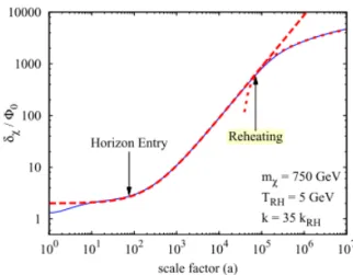
FIG. 1. Demonstration of linear enhancement due to an EMDE for subhorizon modes. Standard logarithmic growth begins at reheating. Figure from Ref. [11]
pair production, with no non-thermal dark matter gener-ation due to scalar field decay. After dark matter freezes out, its comoving number density is conserved. How-ever, during the EMDE, the matter-like scalar field acts as a source to the radiation, and thus additional photons are created. This causes the dark matter-radiation ra-tio to decrease. For the dark matter relic abundance to remain in agreement with current observational bounds from thePlanck mission [12], freeze-out must occur ear-lier, and thus the annihilation cross section hσvi must decrease from the standard value of 3×10⁻²⁶ cm3 s−1. For observations to constrain an EMDE, the boost factor must be sufficiently large to compensate for a lower an-nihilation cross section in order to bring the dark matter annihilation rate above the current observable threshold. The effects from an EMDE on the matter power spec-trum will primarily depend onTRH and the cut-off scale kcut due to dark matter free-streaming. Causally con-nected density perturbation modes grow linearly with the scale factor during the EMDE. When the universe drops below the reheat temperature, the EMDE ends and radi-ation dominradi-ation begins, and evolution of all subhorizon perturbation modes becomes logarithmic until matter-radiation equality. Scales that are larger than the cosmic horizon at reheating (k < kRH) will have experienced no density perturbation enhancement, only growing log-arithmically since horizon entry. Figure 1 demonstrates this behavior for a mode that enters the horizon during an EMDE. Lower reheat temperatures result in a longer EMDE, which allows the density perturbations to grow larger.
sup-pressed due to free-streaming. Ultimately, the modes within the rangekRH< k < kcutwill be enhanced by the EMDE. We first aim to establish the relationship between kRH andkcutas a function of the dark matter mass and the temperatures at reheating and kinetic decoupling.
The post-EMDE matter power spectrum can be used to run cosmological N-body simulations. Given a spe-cific reheat temperature and free-streaming cut-off scale, a power spectrum can be generated and used as input for GADGET-2 [13], a robust cosmological N-body simulator code. This simulates dark matter structure formation on small scales within a cube with side on the order of tens of parsecs/h, running through the cosmic dark ages up until a redshift of zf ∼ 30, allowing us to analyze
in-creased microhalo populations as a result of the EMDE. Analytical models of an EMDE have shown an increase in the fraction of dark matter bound in microhalos from the standard ∼10−10 up to 50% for low reheat tem-peratures. We will use the results of these numerical simulations to verify theoretical results and analyze the structure of individual microhalos.
The focus of this thesis is to determine what happens to these microhalos as the universe evolves. As small microhalos merge with larger microhalos, they may re-main intact as discrete subhalos within the larger host halo. It is also possible that the substructure is destroyed due to these mergers. Microhalo substructure drastically boosts the DM annihilation rate, which is quantified by the boost factor defined as:
1 +Bs=
J
R
ρ2χ4πr2dr
(1)
whereJ is the integral of density squared over the micro-halo volume and the denominator is the integral over a halo with the same mass and virial radius but a smooth density profile. More substructure will cause J to in-crease, in turn increasing the boost factor. If enough substructure has survived in halos, the dark matter an-nihilation rate could be sufficiently boosted for detection using gamma ray telescopes. Of particular interest is the relative boost factor (1 +B)/(1 +Bstd), where 1 +Bstd is the standard substructure boost in annihilation due to subhalos above the reheat scale that form in the absence of an EMDE. Ref. [11] finds that if 90% of the dark matter is still contained in microhalos at z = 50, the relative boost from an EMDE is 100, which is not high enough to overcome the suppression in the annihilation cross section. However, if the microhalos form sufficiently early atz= 400 with 60% of dark matter bound into mi-crohalos at that time, and these mimi-crohalos survive to today as subhalos within a larger host halo, the relative boost factor could be as large as 30,000. This boost fac-tor would be sufficiently high to increase the dark matter annihilation rate in dwarf spheroidal galaxies above the observational limits of theFermi Gamma-Ray Telescope
[14].
The structure of this document is as follows: In Sec-tion II, we use numerical soluSec-tions to a system of coupled
ordinary differential equations [15] to study the evolu-tion of the phase space density of dark matter perturba-tion modes. We will study the perturbaperturba-tion dependence onTRH, Tkd, and dark matter mass mχ. Our ultimate
goal in this section is to construct and verify an analyt-ical model for the free-streaming cut-off scale as a func-tion of the aforemenfunc-tioned temperatures and dark matter mass. We will attempt to determine a set of suitable pa-rameters that result in a cut-off scale small enough to produce sufficient boost in annihilation. Once the rela-tionshipkcut/kRH has been determined, we can generate the matter power spectrum and run cosmological simu-lations, which will be the focus of Section III. We will also employ theRockstar [16] halo cataloging program to find the phase-space coordinates, masses, and radii of all well-resolved, gravitationally-bound structures in the simulation particle data. We will use these halo catalogs to compare the numerical halo mass functions to the an-alytical Sheth-Tormen [17] and Press-Schecter [18] mass functions. For further verification of the simulations, we will fit generalized Navarro-Frenk-White density profiles [19] to simulated halos and compare to analytical pre-dictions for microhalos formed at high redshift. We will also discuss the mass-concentration relationship for mi-crohalos. We will measure the evolution of the bound matter fraction of entire simulations as well as the sub-structure mass percentage of individual host halos. In Section IV, we will calculate the boost factor for micro-halos and generate a boost-mass relationshipBs(Mmh).
This relationship will be integrated over all mass scales below the reheat mass to determine the total substruc-ture boost for galaxy-mass host halos. These total boosts will be compared to observational limits for a given dark matter annihilation cross-section.
Note: Natural units (~ = c = kB = 1) are used
throughout this work.
II. FREE-STREAMING CUT-OFF SCALE
The linear enhancement from an EMDE is only present in modes that enter the horizon before reheating (k > kRH) and modes that are larger than the free-streaming cut-off scale (k < kcut). We seek to understand the de-pendence of the cut-off scale on the dark matter massmχ
and the temperatures at reheating (TRH) and at kinetic decoupling (Tkd).
in Subsec. II C. In particular, we begin by introducing KDEMDE, the code used to study the evolution of the dark matter perturbations, in Subsec. II A. Then, we study the evolution of matter, radiation, and scalar field densities in Subsec. II B. In Subsec. II D, we will focus particularly on numerical effects due to the truncation of an infinite sum that is present due to the boxed terms in Eq. (12). Once we have generated data for the indi-vidual perturbation modes, we will study their relative magnitudes with the “transfer function” in Subsec. II E. Lastly, we will construct an analytical model ofkcut/kRH in Subsec. II F.
A. KDEMDE Introduction and Parameterization
The code to study Eq. (12), KDEMDE, was written by Cosmin Ilie in 2016. The following introduction to numerical evolution of perturbation modes is based on a document written by Cosmin Ilie. The parameters that describe the system are the reheat temperatureTRH, the kinetic decoupling temperature in a standard radiation-dominated (RD) universe TkdS, the dark matter parti-cle speed cχ ≡
p
2TkdS/mχ, and the mode of interest
relative to the mode that enters at reheating k/kRH. Note that the dark matter mass is fixed by the particle speed. The standard kinetic decoupling temperature is reached when the momentum transfer rateγ falls below the Hubble rate in a standard, radiation-dominated uni-verseHRD, and is thus defined byHRD(TkdS) =γ(TkdS). Also, by focusing on the ratio k/kRH, we know that if k/kRH > 1, the mode enters the horizon before reheat-ing, and ifk/kRH<1, the mode enters the horizon after reheating.
The mode that enters the horizon at a particular time is k = R−H1 =aH(a), whereRH is the comoving
Hub-ble radius, as mentioned in the introduction. The mode that enters the horizon at reheating kRH =aRHH(aRH), where the Hubble parameter H ∝ a−3/2 during the EMDE. This is because during the EMDE, the dominant energy source is a pressureless fluid, namely the scalar field, whose energy density ρφ ∝ a−3 and H ∝ √ρφ.
This allows us to set the mode that enters the horizon at reheating askRH≡H1 aaRHI
−3/2
aRH, withH1being the Hubble parameter ataI, the scale factor at the beginning
of the code evolution.
As mentioned above,TkdS, the kinetic decoupling tem-perature in a standard RD background, is defined by:
γ(TkdS) =HRD(TkdS) =
s
8π3 90m2 PL
g∗(TkdS)TkdS4 (2)
with mPL =
p
1/G the Planck mass and γ being the elastic scattering momentum transfer rate between lep-tons and the dark matter. The dark matter remains ki-netically coupled to the radiation whileγ > H. The mo-mentum transfer rate scales asTL4+n, withTL the lepton
temperature and n= 2 in the case of p-wave scattering.
By choosingTkdS, we can then compute the momentum transfer rate as a function of temperature:
γ(T) =γ(TkdS) TL TkdS
!6
(3)
When the radiation is at a particular temperature dur-ing the EMDE, the additional contribution to the total energy density from the scalar field increases the expan-sion rate, sinceH∝√ρ. When compared to a radiation-dominated Universe at the same temperature, the expan-sion rate of the Universe in an EMDE is faster,H > HRD. Therefore, if a standard, radiation-dominated Universe exhibits dark matter-radiation kinetic decoupling atTkdS such that HRD(TkdS) = γ(TkdS), then for the Universe in an EMDE, H(TkdS) > γ(TkdS). Therefore, the dark matter must kinetically decouple at a higher tempera-ture in an EMDE compared to the standard, radiation-dominated case. Ref. [20] finds that the kinetic decou-pling temperature in an EMDE is Tkd ≈ TkdS2 /TRH for TkdS > TRH. We are particularly interested in the case where the dark matter decouples from the plasma dur-ing the EMDE such that the two are not coupled at re-heating, withTkdS > TRH. The radiation perturbations exhibit damped oscillations once the Universe becomes radiation-dominated, and this would also suppress the dark matter perturbations if the two remained kineti-cally coupled after reheating. In the case ofTkdS> TRH, the kinetic decoupling temperature is defined as the so-lution toγ(Tkd) =H(Tkd). In Subsec. II F, we will dis-cuss the implications of an intermediate state between the totally decoupled and fully coupled state termed “quasi-decoupling” [21] and its implications for calcu-lating kcut/kRH. The remainder of our parameters are expressed in terms ofk/kRH, TRH and TkdS.
B. Background Evolution
The KDEMDE code uses a three-fluid model for re-heating [5]:
dρφ
dt + 3Hρφ=−Γφρφ (4)
dρr
dt + 4Hρr= Γφρφ (5)
dρχ
dt + 3Hρχ= 0 (6)
Here, φ denotes the scalar field, r denotes radiation, and χ denotes the dark matter. The rate of radiation production is governed by Γφ, the rate of energy
trans-fer from the scalar field to radiation. While solving this three-fluid system in Eqs. (4)-(6), the initial time tI is
scale factorais the integration parameter, and we move forward with the following dimensionless quantities: ˜ρi=
ρi/ρcrit,1, fori∈ {φ, r, χ} and ρcrit,1 ≡3m2PLH12/(8π) is the critical energy density ataI. In order to reduce
nu-merical instability, the a scaling is absorbed into each of the energy densities so that the quantities become: ¯
ρφ ≡ ρ˜φa3, ¯ρr ≡ ρ˜ra4, and ¯ρχ ≡ ρ˜χa3. We can then
rewrite Eqs. (4)-(6) as: dρ¯φ
da + Γφ
H(a)aρ¯φ= 0 (7)
dρ¯r
da − Γφ
H(a)ρ¯φ= 0 (8)
dρ¯χ
da = 0 (9)
The dark matter temperature,Tχ, obeys the following
differential equation:
adTχ
da + 2Tχ=−2Υ(a)(Tχ−TL) (10) with Υ(a) ≡ γ(T(a))/H(a), and γ defined in Eq. (3). The lepton temperature can be found by solving ρr =
π2
30g∗(TL)T 4
L. We absorb the scaling for the dark matter
temperature with ¯Tχ≡Tχa2. Thus, Eq. (10) becomes:
¯
Tχ0 =−2aΥ(a)( ¯Tχa−2−TL) (11)
C. Perturbation Evolution
With the background ODEs in place, we now introduce the system of coupled ODEs from Ref. [15] necessary to study the evolution of the phase space densityf of each perturbation modek:
dfnl
da + (2n+l)
Υ(a)
a +
R(a) H(a)a2
fnl−2n
R(a) H(a)a2fn−1,l + kcχ
H(a)a2
r
TL
TkdS
l+ 1 2l+ 1
×
(n+l+32) × fn,l+1−nfn−1,l+1
+2l+1l (fn+1,l−1 −fn,l−1)
=δl0
−3dΦ
daAn−2(− dΦ da +
Υ aF∗(ρer)
δr
4 TL
Tχ
)Bn
+δl1 2k 3H(a)a2c
χ r
TkdS TL
(−Φ + ΥH(a)a k2 θr)An
(12) where Φ represents the gravitational potential, θris the
radiation perturbation velocity, and both δl0 and δl1 are Kronecker delta functions. The radiation and scalar
field perturbations follow ODEs that are omitted in this manuscript, but can be found in the appendix of Ref. [5]. To study the dark matter perturbations, we can now employ Eq. (12), noting that we have already made the necessary changes of variables in accordance with our scaling-absorbed terms. In Eq. (12), we use several ad-ditional functions, defined as follows:
R(a)≡ d dτ ln(aT
1/2
L ),
An(a)≡
1−Tχ TL
n
,
Bn(a)≡n Tχ
TL
1−Tχ TL
n−1
,
F∗( ˜ρR)≡
1 + 1 4
dlng∗
dlnTL −1
.
(13)
We can eliminateτ by rewritingR(a) as:
R(a) =H(a)a
"
1 + 1 2TL
dTL
dρ˜r
−4 ˜ρr+
Γφ
H(a)ρ˜φ
!#
(14)
Lastly, we can use dTL
dρ˜r = 1 4
TL ˜
ρrF∗( ˜ρr) to get: R
H(a)a2 = 1 a
"
1 +F∗( ˜ρr)
Γφ
8H(a) ˜ ρφ ˜ ρr −1 2 !# (15)
As previously mentioned,fnl is the dark matter phase
space density, with the density perturbation δχ = f00.
While we are only interested inδχ =f00, the evolution
of this density depends on infinite expansions innandl. The expansion innis a result of the decomposition of the momentum dependence of the dark matter phase space density into eigenfunctions of the Fokker-Planck opera-tor. These eigenfunctions contain a generalized Laguerre polynomial with indexn. The expansion in l is a result of a spherical harmonic in the expanded eigenfunctions. Typically a spherical harmonic includes a second index m, but due to the rotational symmetry of dark matter-lepton scattering, we are only concerned with them= 0 term in the spherical harmonic expansion.
We now have a full model of dark matter perturba-tion evoluperturba-tion that we can explore via numerical calcula-tions. In the simulation code, we will primarily operate under the condition of constantg∗, which is the
param-eter of relativistic degrees of freedom that changes with the plasma temperature.
Two separate versions of KDEMDE are employed in order to separately address the two cases of k/kRH >1 and k/kRH <1. In both versions, the initial scale fac-tor is set to aI = 1. For k/kRH > 1, horizon en-try is fixed at aHOR = 100, and reheating occurs at aRH = aHOR(k/kRH)2. Since this version handles only k/kRH > 1, namely the modes that enter the horizon before reheating, we have guaranteed thataRH > aHOR. Lastly, we set the final scale factor of evolution af =
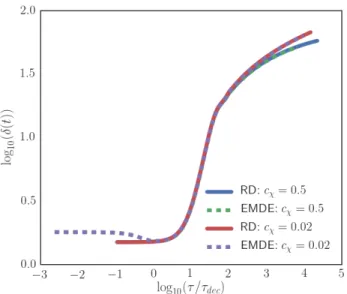
FIG. 2. Comparison between two versions of EMDE code for
k/kRH≈1, where both versions should function properly. At
highercχ, free-streaming suppression becomes noticeable at late times. The rapid decay is due to radiation coupling, as this test case is forTRH> TkdS, andδr→0 at reheating [5].
the mode can evolve sufficiently long for us to observe free-streaming effects and study the time evolution of the modes.
In this case of k/kRH < 1, the user selects the aRH value. The scale factor at horizon entry aHOR can then be found by solving k = aHORH(aHOR). It is impor-tant to note that these modes enter the horizon after reheating, namely aHOR > aRH. This code also evolves the perturbation until af in =nfaRH. As a consistency check, we verify that the results of the two versions of the code agree in the limit ofk/kRH≈1. We evolve a mode out to lowaf = 100aRH, with the density evolutions seen
in Figure 2.
A third version of the code was written that evolves perturbation modes in the absence of an EMDE, assum-ing only radiation domination. We use this version of the code to verify the functionality of KDEMDE for the case of a mode withk/kRH <1. This mode should be unaf-fected by the EMDE since reheating occurs before this mode enters the horizon. Figure 3 demonstrates that KDEMDE does indeed correctly model the evolution of a perturbation mode in the absence of an EMDE. With these consistency checks in place, we can begin testing the evolution limits of KDEMDE.
D. Truncation Analysis
The system of ODEs that govern the evolution of the perturbed dark matter phase-space density is infinite and thus must be truncated in order to numerically solve for f00. Since we cannot numerically evolve an infinite
num-FIG. 3. For a mode that enters the horizon after the EMDE has ended withk/kRH ≈ 0.001, the perturbation evolution
from a code that assumes strict radiation-domination agrees with KDEMDE. Notice the free-streaming suppression at higher values ofcχ.
ber of ODEs, we must choose someNmaxandLmaxabove which we truncate the expansions innandl. As seen in the boxed terms in Eq. (12), truncation error will ini-tially be present in thefNmax,l andfn,Lmax terms for all n ≤ Nmax and l ≤ Lmax. As the perturbation modes evolve, this error will make its way down then, l ladders until it begins to dominate in thef00mode. This means that the truncation error can prohibit accurate pertur-bation evolution to highaf. The first boxed term in Eq.
(12) is proportional tokcχ, so we will not be able to
suc-cessfully evolve out to as high of anaf for largercχ and
k.
In order to generate a matter power spectrum atzi =
2000 for our EMDE simulations, we will need to know the ratiokcut/kRH evaluated today. SinceGADGET-2does not have the capability of simulating the random ther-mal motions of individual dark matter particles in or-der to evolve the free-streaming cut-off scale, the input power spectrum for the simulations must use the value of kcut/kRH evaluated today, rather than evaluated at the redshift where the simulation begins.
FIG. 4. Example of truncation error in the perturbation mode for several values of Nmax. The code begins to break down
at a ≈ 103aRH in this case, but for high k/kRH the error
dominates much earlier.
equation from cosmology:
g∗,eqa3eqTeq3 =g∗,RHa3RHTRH3 (16) In much of our analysis of the perturbation evolutions, we will focus our interests on TRH = 5 GeV. The tem-perature at aeq was approximately 0.75 eV. Lastly, the g∗factor ataeqis 3.91 and at a reheating temperature of 5 GeV,g∗ = 85.6. Thus we expect that in terms of the
reheat scale factor set by the code,
aeq= 1.9×10¹⁰aRH. (17) Unfortunately, this is substantially further out than the code is able to successfully evolve a perturbation mode. By studying the results of KDEMDE for various config-urations ofTRH,TkdS, andcχout toaf between 100 and
1000, we will be able to construct an analytical model of kcut/kRH that agrees with the numerics and predicts out toa0. This discussion will be the focus of Subsection II F.
We are interested in determining theNmax and Lmax that is necessary to evolve a modek/kRH out to a partic-ularaf. We expect that these values ofNmax and Lmax will be sensitive to the particular truncation scheme em-ployed. As a first pass, we define our truncated terms such that:
1. Set both fn,l+1 = 0 and fn−1,l+1 = 0 when l = Lmax
2. Setfn+1,l−1= 0 whenn=Nmax
The effects of truncation can be seen quite clearly in Figure 4. For a perturbation mode that enters only briefly before reheating (k/kRH = 5) with a moderately
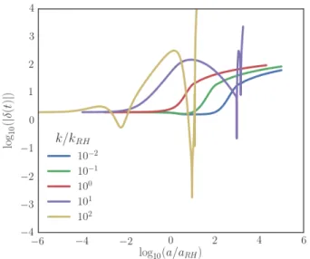
FIG. 5. Evolution and breakdown of various values ofk/kRH
at high cχ = 0.5. For the modes with k/kRH ≥1, the
ini-tial increase inδ(t) occurs due to horizon entry. Note the logarithmic growth after horizon entry as expected.
high particle speed (cχ = 0.5), we see that the truncation
error begins to dominate thef00term at around 103aRH, which allows the mode to evolve sufficiently long for our necessary analysis. Unfortunately, for higher k/kRH, it becomes much more difficult to reach 103a
RH success-fully. By increasingNmax, we are capable of pushing out to further values of af before the error begins to
domi-nate. Unfortunately, asNmax is increased, we begin to see diminishing returns in successfulaf. The point where
continuing to increaseNmaxbecomes computationally in-tractable for analysis of a large parameter space in tem-perature, cχ, and k/kRH is around Nmax ≈ 2000. We note that the code requires a much lower value ofLmax, on the order of 10. For low values of k/kRH, increasing Lmaxpast approximately 15 provides no increase in suc-cessfulaf. This dependence onNmax andLmax seems to reverse at highk/kRH, which will be discussed below.
As mentioned above, the truncation terms in Eq. (12) are proportional tokcχ. Because of this, we expect that
the truncation error will begin to dominate earlier at higherk/kRH. To confirm this expectation, we plot the perturbation evolution for several orders of magnitude of k/kRH in Figure 5. Since the truncation error should in-crease withcχas well, we deliberately use a highcχ= 0.5
so that we study the worst-case scenario, namely the low-est possible af out to which the code can successfully
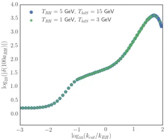
evolve for a givenk/kRH. For k/kRH = 102, we see that the truncation error begins to dominate at an unfortu-nately lowaf ≈10aRH. In order to studykcut/kRH, we will need the code to successfully evolve out to approxi-mately af = 1000aRH and up to k/kRH ≈100. Thank-fully, for the majority of the parameter space that we are interested in,cχ is substantially less than 0.5.
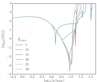
signifi-FIG. 6. At high values of k/kRH, increasing Lmax results
in successful evolution out to higheraf. Here, we are using
Nmax = 1500. We test high cχ = 0.5 to probe the upper
extreme of speeds that we will eventually study.
cantly more sensitive toNmax for lowk/kRH, which can be seen in Figure 4. However, for ln(k/kRH)≈1 to 2, we find that increasingLmax affords an appreciable increase in successful evolution time for largek/kRH modes. This can be seen in Figure 6, where going from Lmax = 5 to Lmax= 30 gains half an order of magnitude of successful evolution for ak/kRH= 100 mode.
Ultimately, we were unable to find truncation schemes that allow for successful evolution out to high af for
ar-bitrarily high cχ and k/kRH. However, our truncation
tests were predominantly for the case of cχ = 0.5, and
we will show below that we will generally be interested in lower values ofcχ. In our discussion of transfer functions,
we find that even with the basic truncation schemes em-ployed above, we manage to evolve the necessary modes out to a range of af between 100 and 1000. For high
values ofk/kRH andcχ, we simply increase the values of
Nmax and Lmax until the mode can successfully evolve out to theaf of interest.
E. Transfer Functions
We now introduce the notion of a transfer function. Fig. 5 shows the perturbation δχ as a function of scale
factor for multiple k/kRH. Suppose that we choose a fixed timeaf and want to know the values ofδχfor each
k/kRH. This is the transfer function, defined as
T(k) =δχ(k) δ0
a
f
, (18)
withδ0 the initial perturbation amplitude at some fixed ai. KDEMDE defines all initial perturbations to have
FIG. 7. Transfer function at 100aRH for cχ = 0.1, and TkdS/TRH= 2. The standard transfer function corresponds to
the expected evolution at 100aRHin the absence of an EMDE.
The post-reheating prediction attempts to match the growth of modes which enter the horizon before the EMDE ends. The difference between this predicted slope and the one seen in the transfer function is likely due to plasma interactions while still coupled atk/kRH> kkd/kRH≈30. The Gaussian
fit is found using Eq. (21).
δ0= 1. We begin ataf= 100aRHand observe the trans-fer function for several orders of magnitude of k/kRH in Fig. 7. The transfer function is calculated using KDEMDE by evolving many modes between 10−3 < k/kRH < 102. The transfer function T(k) relates the matter power spectrum P(k) to the primordial power spectrum generated during inflation ˜P(k) by
P(k) =T(k)2P˜(k) (19) Fig. 7 demonstrates a significant boost due to the EMDE fork > kRH andk < kcut. Here,kcutapproximately cor-responds to the peak of the transfer function, although we will define it more rigorously below. Unfortunately, this power spectrum is only evaluated out toaf = 100aRH,
otherwise the large gap betweenkcutandkRH for a tem-perature ratio as low as TkdS/TRH = 2 would be quite compelling. However, our matter power spectrum is only concerned withkcut/kRHata0. We expect thatkcut/kRH will decrease logarithmically witha, a result that will be confirmed in Subsec. II F with our analytic model.
The post-reheating amplitudes of modes that enter during the EMDE withk > kRH are expected to agree with the following equation from Ref. [11]:
δχ,P R(k > kRH) =
2 3
k/kRH
0.86
2h
1 + lna/aRH 1.29
i
does not quite agree with the results of the numerical sim-ulations, as seen in Fig. 7. The lower slope found in the numerical computations is due to interactions between the plasma and the dark matter that are not modeled in Eq. (20).
We now describe our technique for determining the kcutvalue for a given transfer function. In the absence of free-streaming, the post-reheating transfer function for modes with k > kRH obeys Eq. (20). However, due to free-streaming, modes above the free-streaming cut-off scale are suppressed. We multiply a Gaussian with Eq. (20) to model the peak of the transfer function, with the form:
δχ,Gauss(k > kRH) =δχ,P R(k)e−k
2/(2k2
cut) (21) A demonstration of this fitting can be seen in Fig. 7. It is important to note that the value of kcut determined by the fit is not the peak of the transfer function, but rather the optimalkcut such that Eq. (21) best fits the numerical results from KDEMDE. In order to generate the fit, we use the curve fit routine from the SciPy package for Python. We only use data for k/kRH ≥ 10 for the fit.
After reheating, the Universe becomes radiation-dominated andδχexhibits logarithmic growth after
hori-zon entry for each mode. Ref. [22] provides an equa-tion that describes the transfer funcequa-tion for a radiaequa-tion- radiation-dominated Universe with no free-streaming:
δχ,RD(k) =
10 9 Φ0
h
AlnB a aHOR
i
(22) with A= 9.11, B = 0.594 and in KDEMDE, Φ0= 1.0. For each mode, the scale factor at horizon entry aHOR is defined as the solution tok=aHORH(aHOR). This is the curve labeled “Standard Transfer Function” in Fig. 7.
The values of mχ/TRH that provide the best oppor-tunity for a detectable boost in the dark matter anni-hilation rate are in the range of mχ/TRH ≈ 100−200 [11]. We needmχ/TRH >100 such that the dark mat-ter abundance freezes out during the EMDE, rather than exponentially declining until some later point during ra-diation domination. We would likemχ/TRH <200 such that the annihilation cross section does not become so low as to push annihilation signatures well below the de-tection threshold for the foreseeable future. For a given TkdS andTRH, we can determine the optimum cχ value
to probe thismχ/TRH range by relating cχ to this ratio
as such:
mχ/TRH = 1 c2
χ
2TkdS TRH
(23)
The majority of the work thus far has been done with the temperaturesTkdS = 10 GeV andTRH = 5 GeV, and thus this optimal range of mχ/TRH ratios corresponds to c = 0.14 to c = 0.2. For each temperature ratio, we
FIG. 8. Transfer function atcχ = 0.18 for two different sets of TRH and TkdS, both of which have TkdS/TRH = 3. The
transfer function is agnostic to the actual temperatures, only caring about the ratio.
will have to modulate the values of cχ to fit the
desir-able mχ/TRH accordingly. Figure 8 demonstrates that only the ratio of the temperatures affects the transfer function, and ultimately kcut/kRH, rather than the in-dividual values of TRH and TkdS. We will use transfer functions to explore TkdS/TRH ratios between 2 and 6. Above this, KDEMDE struggles to successfully evolve to high enoughaf to generate transfer functions. We will
construct our analytical model ofkcut/kRHand nail down its dependence onTkdS/TRH,cχ, and af in Subsec. II F,
comparing to all transfer function data available.
F. Analytical Model of Free-Streaming Cut-off
We seek to build an analytical model that can accu-rately predict kcut/kRH for general cχ and TkdS/TRH. Here we provide a derivation of a general form for kcut
kRH. Afterward, we fit the model against our numerical results and discover a remarkable simplification. This simplified model is used to predict thekcut/kRH ata0. Ultimately, we will determine the minimumTkdS/TRH that will pro-vide sufficiently highkcut/kRH to generate significant an-nihilation boosts.
At kinetic decoupling, the dark matter particles begin to free stream. The physical size of the free-streaming horizon lf s = R vχdt. It is important not to confuse
vχ with cχ. Here, vχ is the true physical dark matter
particle speed. Defined in terms of the comoving distance λ, we have that lf s =aλ. We define the comoving
free-streaming horizonλfs such that: λfs≡
Z
dλ=
Z af
akd vχdt
a =
Z af
akd vχ
da
We integrate from decoupling to af, where we choose
af in terms of aRH. We will eventually be interested in
af = a0, namely the scale factor today. The last step
in the equation above comes from the fact that dt =
da da/dt =
da
Ha. The free-streaming horizon λfs corresponds
to a fourth of the free-streaming cut-off wavelengthλcut. Therefore, the free-streaming cut-off wavenumber can be defined in terms of the horizon:
kcut= 2π λcut
= 2π 4λfs
≈ 1 λfs
(25)
In our model, we begin by employing a piecewise func-tional form forH(a) and vχ(a). Using the relationship
thatkRH =aRHH(aRH) =aRHHRH, we have:
H(a) =
bHHRH
a aHt
−3/2
a≤aHt
bHHRH
a aHt
−2
a > aHt
(26)
withaHt= 1.0872aRHcorresponding to the Hubble tran-sition point andbH= 0.882 being a fit parameter. Here,
H ∝a−3/2before the Hubble transition because the Uni-verse is still in a phase of matter domination, whereas H ∝a−2 after the transition because the Universe has transitioned to the radiation dominated era. We define the dark matter velocity using another piecewise form:
vχ(a) = bv qT kd mχ a kd a 9/16
a≤av
bv qT kd mχ akd av
9/16 av
a
a > av.
(27)
The velocityvχ∝ p
Tχ, and Ref. [21] shows that before
the dark matter fully decouples from the radiation, it is in a quasi-decoupled state where Tχ ∝ a−9/8. The
dark matter becomes fully decoupled at av, after which
Tχ ∝a−2. Here,av and bv are fit parameters yet to be
determined. We initially demand that av > aHt which yields three separate pieces for our integral ofλfs, namely the cases where a < aHt, aHt < a < av, and a > av.
Recalling thatcχcontrols our value ofmχ, we can rewrite
our equations forvχ in terms of cχ = p
2TkdS/mχ. We
also need the relationshipTkd=r
T2 kdS
TRH where for constant g∗ as in KDEMDE we have thatr=
p
5/2.
We will also need akd, the scale factor at kinetic de-coupling during the EMDE. This is found with:
aRH akd
=Tkd TRH
8/3h2
5 g∗,RH
g∗,kd
i−2/3
(28)
Once again, we employ constantg∗, and thus g∗,RH = g∗,kd. We can now expressakd,Tkd, and mχ in terms of
our preferred parametersTkdS,TRH, andcχ. The integral
in Eq. (24) is thus split into the three piecewise terms and evaluated. We multiply a factor of kRH onto both
FIG. 9. Using temperaturesTkdS= 10 GeV andTRH= 5 GeV
ataf= 100aRH, this figure demonstrates thec−χ1 dependence
ofkcut/kRH. The model from Eq. (29) is fit to the data points
from transfer function fits of KDEMDE evolutions. The fit values wereav= 1.57aRHandbv= 0.64.
sides and find: kRH
kcut
=kRHλfs = bv bH cχ √ 2r TRH TkdS
5/22
5
3/8aRH
aHt
2516
×
"
16 aHt akd 161 −1 ! +16 7 av aHt 167 −1 !
+av aHt
167 lnaf
av
#
(29) We now have all quantities in Eq. (29) defined except forav andbv. Note that the quantity that we are
inter-ested inkcut/kRH is simply the inverse of Eq. (29). This equation shows two important parameter dependences forkcut/kRH. Firstly, kcut/kRH ∝c−χ1. Ascχ increases,
kcutshould become smaller because the dark matter will be able to travel a greater distance in the age of the Uni-verse. Therefore, larger spatial mode perturbations will be flattened out. Thisc−χ1 dependence is confirmed with
numerical transfer functions from KDEMDE. Secondly, kcut/kRH∝(TkdS/TRH)5/2, so an increase in the temper-ature ratio will greatly increasekcut/kRH.
As a first-pass test of our model, we treat av and bv
as fit parameters. HoldingTkdS/TRH fixed, we plot the numerically-determinedkcut values from the KDEMDE transfer function fits as a function ofcχ in Fig. 9. Using
these data points, we employ a curve-fitting routine to determine the optimumav andbv that best predicts the
kcut/kRHfor allcχvalues at a particular temperature
avandbv from the initial fit are then used to predict the
kcut/kRH forTkdS/TRH = 3 to 5, the model does a poor job of reproducing the numerical results, being off by as much as 25% ataf = 100aRH. Since we are trying to pre-dict out to substantially further times, it is important to have fit parameters that provide a model that agrees to high precision with our numerical results at lowaf. For
example,av/aRH = 1.573 as fit from the TkdS/TRH = 2 data, butav/aRH = 1.223 as fit from the TkdS/TRH = 3 data, introducing a serious discrepancy when attempting to predictkcut/kRHfor a specific temperature ratio when using fit parameters found from another temperature ra-tio’s numerical results. The conclusion is that av and
bv must depend on temperature. Therefore, we seek to
capture this temperature dependence in our model such that the fit parameter values are consistent across differ-ent temperature ratios.
In deriving a model for av and bv, we utilize two key
constraints. Since the temperature of the dark matter particle isTχ∼v2χmχ, we can use constraints on the dark
matter temperature to determine vχ up to a constant,
and then solve for bv. Ref. [23] provides an analytical
model of the dark matter temperature:
TχA(s) =TγsλesΓ(1−λ, s) (30)
withs=αβ2 (akd
a )
αβ,λ= 2−α
αβ, andα= 3/8,β= 4+n−ν.
Here,n= 2 for p-wave scattering andν = 4 in an EMDE. Γ(1−λ, s) is the incomplete Γ-function. The general form of Eq. (28) allows us to solve for the background radiation temperatureTγ:
Tγ
TRH
=h a aRH
5
2
2/3i−3/8
(31) under the use of constantg∗. Since the dark matter
tem-perature is Tχ ∼v2χmχ, we can write Tχ in terms of vχ
from Eq. (27):
Tχ(a) = b2
vTkd
akd
a 9/8
a≤av
b2
vTkd
akd
av
9/8 av
a 2
a > av
(32)
Numerical comparison between the analytical tempera-ture and the true dark matter temperatempera-ture show that, for a aRH, the analytical model of the dark matter temperature TA
χ should relate to the true dark matter
temperatureTχ by:
Tχ(a)(a/aRH)2
TA χ(aRH)
≈1.37 (33)
At early times, for a < 0.1aRH, the analytical tem-perature model is effectively exact, and thus we set Tχ(a) = TχA(a) for a ≤ 0.1aRH. We solve the model
temperature from Eq. (32) ata < av forbv:
bv= s
Tχ(a)
Tkd a akd
!9/16
(34)
Note that since Tχ ∝ a−9/8 before reheating, bv as
de-fined this way is in fact a constant. Sincebv is indeed a
constant, andTχ(a) =TχA(a) fora≤0.1aRH, we can
sub-stitute Tχ(a) for TχA(a) and evaluate bv at a = 0.1aRH,
finding that
bv=
TA
χ(0.1aRH) Tkd
!1/2
0.1aRH akd
!
, (35)
where akd comes from Eq. (28). We introduce a new prefactor d2v to the definition of Tχ(a) in Eq. (32) to
assuage the ambiguity fromTχ ∼v2χmχ. With the above
form forbvand the addition of the newdvparameter, we
can now solveTχ at a > av forav, using the constraint
from Eq. (33) to replaceTχ(a) foraaRH, finding:
av = "
1.37TA
χ(aRH)a2RH d2
vb2vTkda 9/8 kd
#8/7
. (36)
We can now combine all of this for our final model, which only depends on our temperatures,cχ, and our fit
parameterdv:
kcut kRH
=
"
bvdv
bH cχ √ 2r TRH TkdS
5/22
5
3/8aRH
aHt
2516
×
(
16 aHt akd 161 −1 ! +16 7 av aHt 167 −1 !
+ av aHt
167
lnaf av
)#−1
(37) Using transfer function data for af = 100aRH at fixed TkdS/TRH, we fit the model to determinedv. At the same
temperature ratio, we then use the completed model with the dv fit at af = 100aRH to predict kcut/kRH at af = 200aRH, 500aRH, and 1000aRH compared to those from KDEMDE. This allows us to draw an interesting conclusion: using only thedvfit from the KDEMDE data
ataf = 100aRHacross many values ofcχ, we find that as
af increases, the difference between our model and the
numerical KDEMDE value ofkcut/kRH decreases. This is remarkable, as it implies that were we to evolve per-turbation modes out toa0 using KDEMDE, the model would be able to accurately predict the free-streaming cut-off mode. The late-time constraint on the tempera-tures from Eq. (33) is accounted for in av and ensures
that we accurately capture the temperature evolution at late times. This is important because the integral to calculateλfs is dominated by the contribution from late times, which is encoded in the boxed, logarithmic term in Eq. (37).
Unfortunately, the values of dv from fits of the
kcut/kRH vs. cχ relationship do not agree across
differ-ent temperature ratios. Note that av depends on both
TABLE I. Comparison between the fit parameter dv for the two different functional forms of bv. The column labeled “Earlydv” shows fit values ofdvwithbvdefined in Eq. (35). The column labeled “Late dv” shows fit values of dv with
bv as defined in Eq. (39). The fits were made against the
kcut/kRH vs. cχ relationship data from KDEMDE taken at af = 100aRH. The reduced fluctuation indvfor the late-time
dependent bv of Eq. (39) demonstrates that this form ofbv
matches the temperature dependence better.
TkdS/TRH Earlydv Latedv
2 1.350 1.024 3 1.259 1.035 4 1.268 1.066
we find that the model fits best for dv values that push
av/aRH to high values upwards of 40. The largeav/aRH ratio indicates that the model is artificially suppressing the first two additive terms in Eq. (37) in favor of the third, boxed term of our piecewise integral ofλfs. This suggests that the post-reheating behavior dominates the calculation ofkcut/kRH. This motivates us to make a re-markable simplification to the model. Since the late-time behavior dominates the calculation ofkcut/kRH, the first two terms in Eq. (37) become negligible compared to the third term as af increases. Therefore, we choose to
simply drop the first two terms. We setav =aRH and consider the model:
kcut kRH
=
"
bvdv
bH cχ √ 2r TRH TkdS
5/22
5
3/8aRH
aHt 2516 × ( aRH aHt 167 ln af
aRH
)#−1 (38)
wheredv now functions as the overall normalization
pa-rameter and we expressbv in terms ofav=aRH by solv-ing Eq. (36) forbv:
bv= s
1.37TA
χ(aRH)a2RH a7RH/8Tkda
9/8 kd
(39)
This formulation ofbv incorporates our late-time
con-straint from Eq. (33). With the simplified model in Eq. (38), we can go back to fitting data in thekcut/kRHvs. cχ
relationship such as in Fig. 9. Withav =aRH and only one free parameterdv, we can now compare the two
dif-ferent definitions ofbv in Eqs. (35) and (39). We fit the
simplified model to thekcut/kRHvs. cχ data for multiple
temperature ratios and display the fitting parameters in Table I.
Table I shows a strong improvement of the model by using the one-part integral and bv defined in Eq. (39).
The reduced fluctuation in the near-unity fitting param-eter with this definition of bv shows that the functional
form of bv better captures the temperature dependence
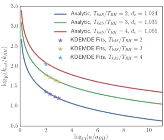
at late times than that of Eq. (35). As demonstration of the predictive power of the model under this new for-mulation, in Figure 10 we look at the time evolution
FIG. 10. For fixed cχ = 0.1, we use the analytical model in Eq. (38) with bv as defined in Eq. (39) to predict the time evolution ofkcut/kRH. For several temperature ratios,
we compare this time evolution to that found via KDEMDE for the corresponding sets of parameters. The ratios are ex-trapolated out toaeq∼1010aRH.
ofkcut/kRH for several temperature ratios and compare to the time evolution from KDEMDE. This figure high-lights the expected logarithmic decrease ofkcut/kRHwith af. When assessing temperature ratios greater than 4,
we have no data from KDEMDE to make a fit for dv.
Fortunately, as demonstrated by the “Latedv” column
of Table I, the fit parameter is nearly constant across temperature ratios. For this reason, predictions made for TkdS/TRH > 4 can be made using the dv fit from
TkdS/TRH= 4 with minimal loss in accuracy due to fluc-tuations indv.
Since we have completed our model fitting by consid-eringaf aeq, we can now incorporate the final term in
the model that is evaluated fromaeqtoa0. Once matter domination begins, the Hubble rate becomes:
H(a) =bH kRH
aRH
aHt
aeq
2aeq
a
3/2
a≥aeq. (40) However, the dark matter velocity remains unchanged from Eq. (27). We evaluate the integral in Eq. (24) as previously done out toaeq, with the simplified model in Eq. (38). However, we now add an additional term resulting from the evaluation of the integral fromaeq to a0, such thatkcut/kRH evaluated today is:
kcut kRH
=
"
bvdv
bH cχ √ 2r TRH TkdS
5/22
5
3/8aRH
aHt 2516 × ( aRH aHt 167
lnaeq aRH
+ 2aRH aHt
7/16
1−
ra
eq a0
)#−1
.
The contribution to this calculation from the period be-tween matter-radiation equality and today is dwarfed by the contribution between reheating and matter-radiation equality. Now that we are comfortable with our model, we can determine the temperature atcχparameters that
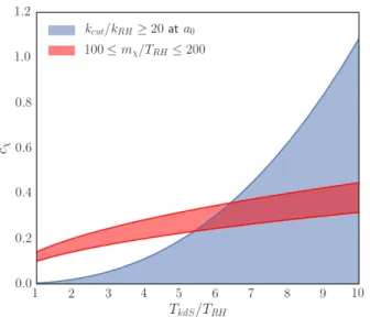
will provide this sufficiently high kcut/kRH ata0. In or-der to generate a dark matter annihilation boost suffi-cient to overcome the reduced annihilation cross section, we need at least kcut/kRH ≈ 20 [11]. Figure 11 shows the parameter space of the temperature ratio and cχ
that have kcut/kRH ≥ 20 at a0. Dark matter particles with mχ/TRH in the range 100 to 200 are most capa-ble of having their annihilation rate boosted above the current minimum sensitivity threshold of missions such as theFermi Gamma-Ray Telescope. Since dark matter typically freezes out before it kinetically decouples, we must also demand that the freeze-out temperatureTf be
greater than Tkd. According to Ref. [11], dark matter typically freezes out when mχ ∼ 10T. This demands
thatTf/TRH∼0.1mχ/TRH.
Unfortunately, TkdS/TRH = 6 is the lowest tempera-ture ratio that giveskcut/kRH≈20 ata0 formχ/TRH≤ 200. In this case, Tkd ≈ 9TkdS ≈ 54TRH. For our up-per bound mχ/TRH = 200, we have thatTf/TRH ≈20. Clearly,Tkd> Tf, which is not consistent with the stan-dard theories of dark matter formation. The other possi-ble scenario that would providekcut/kRH≈20 ata0with a lower temperature ratio that remains consistent with standard theories would require that mχ/TRH 200, resulting in heavy suppression of the annihiliation cross section that would push dark matter annihiliations be-low the observable threshold for any mission in the near future [11]. We are interested in studying the sce-nario where the EMDE could have potential constrain-ing power on the dark matter particle, and thus we will choose our parameters to be TkdS/TRH = 6 and cχ = 0.245. With these parameters, we can generate a
matter power spectra with the necessarykcut/kRH = 20, to be done in the next section.
III. COSMOLOGICAL SIMULATIONS
In this section, we study the evolution of a universe that undergoes an EMDE withkcut/kRH = 20. We start out by generating the matter power spectrum for this universe that represents the enhanced perturbations on modes kRH < k < kcut. This power spectrum will be transformed into initial condition data for theGADGET-2 cosmological N-body simulator code [13]. We run the simulation at multiple scales in order to study a larger range of masses and confirm convergence between the simulations. The N-body simulator returns only the phase-space data of all particles in the code. This parti-cle data is piped through theRockstar[16] halo finder to determine the location and radius of all gravitationally-bound structures in the simulation. We employ the con-vention that the halo radius is that which makes the
av-FIG. 11. Using the model ofkcut/kRH from Eq. (38) and
the convergedbv = 1.770 from Eq. (39), we find the maxi-mum value ofcχfor each temperature ratio that will provide akcut/kRH ≥20 at a0. This is compared to the desired
pa-rameter space of 100 ≤ mχ/TRH ≤ 200. Note that for a
given temperature ratio, a lowercχ corresponds to a higher
mχ/TRH.
erage halo densityρhalo= 200ρc, whereρc is the critical
density of the universe.
With these halo catalogs collected, we can determine some macroscopic statistics about the halo populations from the simulation. The halo mass function describes the number density of dark matter halos per mass inter-valdn/dlnM. We compare these results to the Press-Schecter [18] and Sheth-Tormen [17] formalisms.
We then briefly discuss the total bound matter fraction in the simulation as a function of redshift z. As time progresses, we expect that the total amount of matter bound into structure will increase. This can be verified by generating a halo catalog for each simulation snapshot and determining the total mass in structure compared to the total mass simulated in the box. Similarly, we look at the total fraction of matter bound in substructure per halo as a function of host halo mass.
profile and fit it against the generalized Navarro-Frenk-White (NFW) profile [19]. To calculate the halo boost factor of each halo as in Eq. (1), we use the NFW profile for a standard reference halo in a process described in Subsection III E. We conclude this section with all the necessary groundwork laid to calculate the boost factor of every halo in the simulation and continue forward by analyzing the statistical properties of these boosts.
Many of the aforementioned processes are repeated for an identical universe that still has a free-streaming cut-off scale but lacks an EMDE. See the “Only FS cut-cut-off” curve in Fig. 12. These “standard” simulations serve as a useful control to demonstrate the boost due to the EMDE in the EMDE simulations.
A. Power Spectra and Simulation Parameters
With an enhanced region of wavenumber-space now determined such thatkcut/kRH = 20, we create a power spectrum for a universe that undergoes an EMDE and re-heats atTRH= 30 MeV. This power spectrum is related to the transfer function of each individual mode accord-ing to Eq. (19), where the primordial power spectrum
˜
P(k) comes from observations of the cosmic microwave background. The other component of the power spec-trum, the transfer function Tzi(k), is calculated using the collisionless Boltzmann equation by determining the density perturbation of each wavenumber at the start-ing redshift of the simulation, as in Subsec. II E. This power spectrum is used as the input to the UniGrid routine, which randomly generates density perturbations δχ(~x, zi) that obey the statistical properties demanded by
the power spectrum. Here, the zi simply indicates that
the perturbations are at the initial redshift where the N-body simulation begins the evolution. Thisδχ(~x, zi) data
is then piped throughDelta2Particles, which generates the initial coordinate and momentum data for all the par-ticles in the simulation. TheGADGET-2N-body simulator takes this initial particle configuration and simulates the gravitational evolution up until a desired final redshift. Throughout this work, we use the cosmological parame-tersh= 0.678, Ωm= 0.309, Ωb= 0.049, and ΩΛ= 0.691 in accordance with the 2015 results fromPlanck [12].
In order to study the evolution of microhalos with an N-body simulation, we must be diligent to ensure that the mass resolution of the simulation is sufficient to re-solve the microhalos. The EMDE only alters structure on mass scales below the reheat massMRH, which is the mass enclosed in the Hubble radius at reheating. The Hubble radius R = 1/(aH), and k ≈ R−1 up to order unity. Therefore, the mass enclosed in the Hubble radius at reheating is
MRH= 4 3πρmR
3 RH=
4 3πρmk
−3
RH. (42) SincekRHis a comoving quantity,ρmis simply the matter
density today. A convenient expression for the reheat
FIG. 12. The matter power spectrum atz = 500: the solid curve extrapolates results from the Planck 2015 mission [12]; the dash-dotted curve uses the same data from Planck but contains a free-streaming cutoff withkcut/kRH= 20 in a
uni-verse with reheating atTRH = 30 MeV; the dotted curve is
the power spectrum of a universe with an EMDE, where the enhanced region rises above the standard power spectrum for modes bounded bykRHandkcut.
mass in terms of the reheat temperature is:
MRH = 32.7M⊕
10 MeV
TRH
3g∗s[TRH]
10.75
10.75
g∗[TRH] 3/2
.
(43) The two key simulation parameters that determine the individual particle mass are the particle count and the box size. The number of CPU hours required to complete a simulation roughly scales with the particle count, and for this reason we choose Npart = 10243 particles such
that each simulation takes on the order of 104CPU hours. We select small box sizes of (30 pc/h)3, (60 pc/h)3, and (120 pc/h)3. These simulation configurations result in particle masses of 2.16×10⁻¹²M
/h, 1.73×10⁻¹¹M/h,
and 1.38×10⁻¹⁰M
/h, respectively. The combination of
large particle count and small box size allows us to probe a rather low mass regime. We briefly note that we also employ an even smaller 1 (pc/h)3 simulation exclusively to study high resolution density profiles. See Subsection III E for our discussion on this topic.
TheRockstarhalo finder only catalogs halos above a certain minimum particle count, which we select to be 100 particles. Therefore, our 30 pc/h simulation has a minimum halo mass of 2.16×10⁻¹⁰ M
/h. Referring
back to Eq. (43), we see that for a reheat temperature of TRH = 30 MeV, the reheat mass is MRH = 3.5 × 10⁻⁶ M
, or approximately one Earth-mass. For this
consideringkcut/kRH= 20, the cut-off mass is a factor of 203 smaller than the reheat mass.
This low reheat temperature was chosen so that we could resolve microhalos in the mass regimeMcut< M < MRH for our given simulation parameters. A higher re-heat temperature will push the microhalo formation to increasingly small mass regimes that are more inaccessi-ble to an N-body simulator. However, it is important to recall from Section II that only the ratio TkdS/TRH af-fects the transfer function and thus the power spectrum. The primordial microhalos will form at approximately the same redshift regardless of the reheat temperature, with formation time only depending onkcut/kRH. For a fixed ratio of kcut/kRH, the first microhalos to form will all have approximately the same density, whereas the size of the microhalo clumps will depend on TRH. Ref. [11] demonstrates that regardless of reheat temperature, the differential bound mass fractiondf /dlnM remains fixed relative to the reheat mass. With this fixed relative dif-ferential bound mass fraction and the consideration that all primordial microhalos form at the same density, we expect the annihilation boost to not be sensitive toTRH. Therefore, the following results are general to higher re-heat temperatures.
In order to capture the formation of low-mass micro-halos in the simulation, the EMDE simulations begin at a zi = 2000. Since this redshift is fairly near the
point of matter-radiation equality, effects due to radia-tion are still significant. Unfortunately, GADGET-2 does not presently have radiation physics incorporated, and thus we are unable to model the effects due to radiation. To mitigate this, the input power spectra are generated for z = 500, where radiation effects are negligible, and integrated back tozi= 2000 assuming only that the
Uni-verse is entirely matter-dominated. This way, when the simulation evolves from a redshift of 2000 to 500, the power spectrum will be accurate atz= 500, and the re-maining evolution of the simulation can continue forward without the need for radiation physics. The simulations that evolve without an EMDE but with a free-streaming cut-off begin atzi= 500. The N-body simulator evolves
the code up to zf = 30 and takes 10 snapshots of the
particle data along the way at equally-spaced intervals in scale factor. These snapshots will be used to study the total bound mass fraction in Subsection III C.
B. Halo Mass Functions
The majority of our subsequent analysis focuses on the final snapshot data from GADGET-2 at zf = 30. This
particle data is sent through Rockstar to find all ha-los of particle count greater than 100. We are inter-ested in verifying the microhalo populations of our sim-ulations against established theory. The Press-Schecter mass function [18] is an analytical formalism that pre-dicts the number density of halos as a function of mass
interval, defined as: dn
dlnM =
r
2 π
ρmδc
M σ(M, zf)
exph− δ 2
c
2σ(M, zf) i
dlnσ dlnM
(44) where δc = 1.686 for z & 2 is the critical linear
over-density, ρm is the matter density of the Universe today,
andσ(M, zf) is the rms density perturbation in a sphere
that contains a massM: σ2(M, z) =
Z d3k
(2π)3[D(k, z)T(k)] 2P
p(k)F2(kR) (45)
whereD(k, z) is the scale-dependent growth function [5], T(k) is the transfer function,Pp(k) is the power spectrum
of super-horizon density perturbations during radiation domination, and
F(kR) = exph−k 2(αR)2
2
i
×2[sin(kR)−(kR) cos(kR)] (kR)3
(46) with α = 0.0001 and R = [3M/(4πρm)]1/3 (Refs. [11]
and [5]).
A similar model of the halo mass function was con-structed by Sheth & Tormen [17]:
dn
dlnM = 0.3222× ρm
M
dlnσ dlnM
s 2 √ 2π ×h1 +
√
2σ(M, zf)
δ2
c
0.3i δc
σ(M, zf)
exph− √
2δc2 4σ2
i
(47)
In order to calculate the mass functions from the nu-merical data, we extract from the Rockstar halo catalog an array of the masses of all host halos, namely only the ones that have no parent halo in the substructure tree. Then, the halos are binned by mass using an adap-tive binning routine so that for a simulation withNh,tot hosts, the minimum number of halos in a bin is
FIG. 13. Comparison between mass functions from numerical simulations and the predictions made by the Press-Schecter (Eq. (44)) and Sheth-Tormen (Eq. (47)) mass functions. The numerical data is taken at zf = 30 for six different 10243 particle simulations. The three numerical curves that are of larger magnitude in dn/dlnM correspond to the EMDE simulations, whereas the lower magnitude curves correspond to the standard simulation without an EMDE. The vertical lines correspond to the minimum halo size of 100 particles for the corresponding simulation. Note that the standard and EMDE mass functions are nearly converged at the reheat massMRH= 3.5×10⁻⁶ M. The enhanced level of structure formation due to the EMDE is clear from the large difference indn/dlnM betweenMcut< M < MRH.
functions begin to converge such that the EMDE plays no role in higher mass structure formation, and this is indeed confirmed by the numerical mass functions. The figure also demonstrates that the simulation results are reason-able, as the mass functions are in fairly good agreement with the analytical predictions. We find that the Press-Schecter mass function is a better predictor of microhalo number density in the EMDE simulation, whereas the Sheth-Tormen mass function is a more accurate model of the microhalo number density for a universe that evolves in the absence of an EMDE. The Press-Schecter mass function considers spherical collapse of dark matter ha-los whereas the Sheth-Tormen mass function considers elliptical collapse. The stronger agreement between the Press-Schecter mass function and the results from the EMDE simulation suggests that structure collapse could be more spherical for EMDE-generated microhalos. We now shift our attention to subhalo mass statistics and the evolution of the total bound matter fraction with redshift.
C. Bound Matter Fraction and Substructure Mass Fraction
For a given halo, its substructure mass fraction fs is
defined as the total amount of mass bound in subhalos
relative to the total mass in the host halo: fs=
P iMsub,i Mhost
(49) where i runs over all subhalos, Msub,i is the mass of a particular subhalo, and Mhost is the total mass of the host halo. We are interested in the statistical properties of this quantity as a function of host halo mass.
In Figure 14, we study the substructure mass frac-tion across several redshifts and compare the result at zf = 30 between the EMDE simulation and the standard
radiation-dominated simulation. As expected, there are substantially more total host halos in the EMDE simu-lation at zf than there are in the standard simulation.
In fact, the difference is about a factor of 42, with ap-proximately 106,000 hosts in the EMDE simulation and only 2,500 in the standard simulation. This is readily apparent from the aforementioned halo mass functions. As the EMDE simulation evolves, we can see that higher mass host halos begin to contain substructure. At high redshift, the majority of halos havefs = 0. We also see
that the total number of substructure-less host halos de-creases as time inde-creases. In particular, atz= 186, over 96% of halos contain no substructure. Byzf = 30, only
(a) Redshift evolution of the substructure mass fraction for a universe that undergoes an EMDE. Atz= 186, over 96% of halos contain no substructure. Byz= 114, only 91% of halos contain no substructure.
(b) On left: continued redshift evolution of EMDE simulation. Byz= 30, 85% of halos contain no substructure. On right: When contrasted against a simulation that undergoes standard radiation domination, only 71% of halos contain no substructure atz= 30.
However, hosts are substantially more abundant in the EMDE simulation by a factor of 42.
FIG. 14. Substructure mass fractions for a 10243 particle, 60 (pc/h)3 box simulation. The first three images depict redshift evolution and the final image compares the results atzf = 30 between the standard simulation and the EMDE simulation. The green curve represents the minimum possible fraction that one single 100 particle subhalo can contribute to the total host halo mass. Fractions greater than 1 are possible due toRockstar’s subhalo identification technique: only the center of a subhalo must be within the host haloR200 radius.
of total host halos increases temporarily and then begins to decrease after the sub-reheat mass halos stop form-ing and begin to merge. At z = 186, there were 76,000 hosts, which increases up to 140,000 by z = 114. How-ever, these microhalos begin to merge and by zf = 30
there are only 106,000 host halos. We expect that this trend would continue if lower redshifts were probed. The general trend from Fig. 14 is that as the more massive halos begin to form, they do so by merging with smaller halos. At first glance, the data in Fig. 14 appears quite
dense and could be masking a trend. However, after in-spection with a Hess diagram, we report that there is no trend forfsversusMhost. Unfortunately, the simulation resolution limits our ability to fully study this relation-ship. In order forRockstarto identify a subhalo within a host halo, the subhalo itself must contain at least 100 particles. The curves in Fig. 14 track the value offsfor
FIG. 15. The differential bound fraction given by Eq. (50) at zf = 30. On left: df /dlnM from the EMDE simulations. On right: df /dlnM from the standard simulations. Note the large boost indf /dlnM due to the EMDE as compared to the standard simulation.
have substructure that is not resolved by the simulation. If a higher resolution was used, it may be possible to fur-ther explore the fs−Mhost relationship in search of a trend.
We now introduce the differential bound fraction of dark matter. Recall that the halo mass function is dn/dlnM and describes the dark matter number den-sity as a function of mass bin. The differential bound fraction describes the fraction of the total dark matter that is bound into a particular mass bin. We denote this quantitydf /dlnM and it follows directly from the mass function:
df dlnM =
dn dlnMVbox
M Mbox
(50) withMbox=NsimMp. Here,Mpis the mass of a particle
andNsim= 10243 particles in the simulation. Note that
dn
dlnMVbox = dN
dlnM, the differential halo count per mass
bin. Clearly, the factor ofM/Mboxtransforms this quan-tity into a mass fraction, with M located at the center of each corresponding mass bin. Since we have already calculated our mass functionsdn/dlnM in Subsec. III B, it is simple to calculate df /dlnM. In Fig. 15, we plot the differential bound fraction for both the EMDE and standard simulations. This result is consistent with pre-dictions from Press-Schecter [18]. The differential bound fraction of a universe that evolved with an EMDE peaks at approximately M/MRH ≈ 10−2 at z = 30. We also see that, as expected,df /dlnM is substantially lower for the standard simulation. Note that the level of disagree-ment between the three different box sizes is in fact quite small and only due to resolution effects. When compared with the great convergence seen between the various mass functions of Fig. 13, we point out that the mass functions were plotted in logarithmic space, whereas df /dlnM is only in linear space. Therefore, any lack of convergence due to resolution in the mass functions is obscured where
it is otherwise apparent indf /dlnM. Nonetheless, we are satisfied with the level of convergence demonstrated.
Of particular interest is the integral of df /dlnM up to the reheat mass, namely the total bound fraction in sub-reheat mass halos:
ftot(zf) =
Z lnMRH
lnMcut df dlnM
z
f
dlnM. (51) We are interested in the total bound fraction as a func-tion of redshift. Rather than numerically integrate the df /dlnM curves from Fig. 15, ftot can be calculated directly from theRockstarhalo catalogs with:
ftot =
PM <MRH
i Mhost,i Mbox
(52) whereiruns over all host halos with mass below the re-heat mass as identified by Rockstar and Mhost,i is the mass of each host. Analytical models of an EMDE pre-dict that the fraction of dark matter bound in microhalos may increase by several orders of magnitude for a reheat temperature as low as TRH = 30 MeV when compared to structure formation in the absence of an EMDE [11]. Figure 16 demonstrates the redshift evolution offtot for both a universe that experiences an EMDE and a stan-dard universe. As predicted, the fraction of dark matter that is bound in microhalos is substantially higher due to an EMDE at nearly 70% atzf = 30. Ideally, we wish to
calculateftotat lower redshifts. This is unfortunately not possible since our simulation stops atzf = 30. We expect

![FIG. 12. The matter power spectrum at z = 500: the solid curve extrapolates results from the Planck 2015 mission [12];](https://thumb-us.123doks.com/thumbv2/123dok_us/8334677.2212053/15.918.476.823.98.384/matter-power-spectrum-solid-extrapolates-results-planck-mission.webp)

