DEVELOPMENT PATTERNS AND
MUNICPAL FINANCES
A
N
A
NALYSIS OF
S
PRAWL AND
S
PENDING IN
82
U.S.
C
ITIES
PATRICK WELCH
UNIVERISTY OF NORTH CAROLINA-CHAPEL HILL Department of City and Regional Planning
WELCH 1
T
ABLE OFC
ONTENTSABSTRACT 2
I. INTRODUCTION 3
II. DEFINITIONS 4
WHAT IS SPRAWL? 4
Figure 1. The four elements of sprawl: Leapfrog development, commercial strip development,
low-density and single-use development. 5
MEASURING SPRAWL IN THE UNITED STATES 6
III. THE IMPACTS OF SPRAWL 8
SPRAWL INDEX 12
Table 1. The most and least sprawling cities in 2010. 14
Figure 1. Map of change in sprawl index from 2000-2010. 15
MUNICIPAL EXPENDITURES 15
Figure 2. Change in per capita total direct expenditure (2000-2010) in 2012 dollars. 18
CONFOUNDING FACTORS 18
Table 2. Descriptive Statistics for Key Variables. 19
Figure 4. The 82 selected cities included in study. 20
REGRESSION MODELS 20
V. RESULTS 22
Figure 5. Scatterplot of relationship between sprawl index and per capita direct expenditures
(2000-2010). 23
Figure 6. Summary of the regression results in the 13 significant models. 24
VI. DISCUSSION 26
REFERENCES 30
APPENDIX 32
APPENDIX A. SPRAWL INDEX CALCULATIONS FOR THE 82 SELECTED CITIES. 32
APPENDIX B. KEY FINANCIAL DATA FOR SELECT CITIES. 33
WELCH 2
A
BSTRACTSprawl has long been lamented in urban planning circles for its detrimental
environmental, social, and financial impacts. However, most of the widely cited literature use
theoretical models to measure the financial impacts and inefficiencies of sprawling development.
This paper examines the relationship between sprawl and municipal finances empirically, by
analyzing 23 separate financial categories in 82 of the largest cities in the United States between
the years 2000 and 2010. First, the concept of sprawl is defined and a brief overview of existing
literature on the impacts of sprawl is presented. Then, 23 separate multivariate regression
models are created and analyzed using a sprawl index calculated by Hamidi and Ewing (2014) to
predict each of the financial categories, including various expenditure categories, debt
outstanding, and capital outlay. In line with existing literature, the research finds that there is a
significant and negative relationship between sprawl and capital outlay expenses. More compact,
accessible cities spend less on capital outlay. The findings indicate that urban form and land use
patterns have serious financial implications and that cities should consider investments in
WELCH 3
I.
I
NTRODUCTIONFrom glancing at the local issues section of any local newspaper, it may seem like two new
crises are threatening towns across the nation: density and sprawl. Headlines such as
“Homeowners fear high-density zoning” (Levenson 2015), “Residents fear housing density”
(Gonter 2008), and “Residents fear ‘urban sprawl’” (Sholtis 2016) highlight the contentious
debate that often surrounds new developments. The terms “high-density” and “sprawl” have
been demonized and used to attack new development proposals by conjuring up images of either
Manhattan-like skyscrapers or a suburban wasteland void of natural elements in order to foster
public outrage. These arguments appeal to residents’ and local politicians’ emotions, while
ignoring the facts of what “density” and “sprawl” actually are and their implications, both positive
and negative. Both “sprawl”, and its adversary “density”, carry serious environmental, social, and
economic consequences that should be evaluated carefully by decision-makers. This paper aims
to shed light on some of these issues, specifically the financial impacts bore by cities and service
providers, in order to provide much needed empirical evidence to a debate that is full of
WELCH 4
II.
D
EFINITIONSW
HAT IS SPRAWL?
First, it is important to establish a clear definition of sprawl, while also gaining a better
understanding of its presence in American cities. Sprawl is widely considered an American
phenomenon, promulgated by widespread automobile ownership, cheap land, and poor
planning (Hamidi and Ewing 2014). But a true objective definition is often missing in
conversations. For example, take the following definitions of sprawl by several well-known
organizations:
• The Sierra Club: “Sprawl—scattered development that increases traffic, saps local resources and destroys open space.”
• Natural Resources Defense Council: “Sprawling development eats up farms, meadows, and forests, turning them into strip malls and subdivisions that serve cars better than people.” (Poland, CPBG)
These definitions are problematic because they define sprawl in terms of their negative
outcomes, rather than the objective characteristics of sprawl. They also define sprawl using
words that carry negative connotations, further emotionalizing the debate. Ewing (1997) offered
one of the first objective and comprehensive definitions of sprawl that is still used widely today.
He defines sprawl as having one or more of the following four elements:
1. Leapfrog or scattered development,
2. Commercial strip development,
3. Expanses of low-density development, and
WELCH 5 An additional indicator of sprawl that Ewing established was poor accessibility – large areas of
vacant land separating uses, poor linkages with transportation networks, and a dependence on
the automobile. For this paper, I will use Ewing’s definition of sprawl, as it is still one of the most
comprehensive definitions that attempts to consider the many complex elements of sprawl.
But what is the difference between sprawl and suburbanization? Unfortunately, in the
United States they are often one in the same, but this is not necessary. One of the main elements
of sprawl is that it is suburbanization that occurs rapidly without careful planning, leading to a
WELCH 6 patchwork of low density, single-use development arranged around the automobile.
Suburbanization in the U.S. all too often follows this pattern, but it is possible for suburbanization
to occur in a deliberate, planned fashion that does not result in urban sprawl. In fact, many cities
in the United States have actively managed to grow without sprawling uncontrollably.
M
EASURINGS
PRAWL IN THEU
NITEDS
TATESMuch of the literature on urban sprawl focuses on its definition and how to accurately
measure it. Scholars have long had a difficult time differentiating sprawl from suburbanization
(Carruthers and Ulfarsson 2003). Early measurements of sprawl focused on density, with lower
densities being more sprawling areas (Pendall 1999). While these calculations were critiqued for
not capturing the full idea of sprawl, they were very easily calculated from readily-accessible
data. As technology advancements made satellite imagery cheaper and more available to the
public, new measurements of sprawl emerged that tried to account for other dimensions beyond
density, including fragmentation (leap-frog development) and edge density (Huang, Lu, and
Sellers 2007). The most advanced measures of sprawl consider sprawl’s multidimensional nature
and combine multiple factors into a single sprawl index. One of the most widely cited sprawl
indices was developed by Smart Growth America in collaboration with the U.S. Environmental
Protection Agency (Ewing et. al. 2000). This sprawl index takes into account four different
indicators of sprawl, with an average score of 100 for each indicator. The indicators directly relate
to Ewing’s definition of sprawl mentioned earlier and include: residential density; neighborhood
mix of homes, jobs, and services; strength of activity centers and downtowns; and accessibility
WELCH 7 overall sprawl indicator. While these indices are more robust and better capture the complexity
WELCH 8
III.
T
HEI
MPACTS OFS
PRAWLWhile the literature on how to define and measure sprawl varies greatly still, the negative
impacts of sprawl are widely cited. Increased traffic fatalities, physical inactivity, obesity, air
pollution, extreme heat events, energy use, commute distances and times, and social capital have
all been shown to worsen because of sprawl (Hamidi at. al. 2015). Other research has tried to
connect sprawl to positive benefits, such as increased homeownership, affordable housing, and
more open space (Glaeser and Kahn 2004). This project, however, will focus on the financial
impacts of sprawl on municipal governments and service providers, rather than the
environmental and social costs.
One of the most widely-cited and reviewed studies on sprawl and its associated service
provision costs was conducted by the Real Estate Research Corporation in 1974. This study,
commissioned by the Environmental Protection Agency, the Department of Housing and Urban
Development, and the U.S. Council on Environmental Quality, examined the impact on
infrastructure costs for six hypothetical communities of 10,000 housing units with different
densities. The explanatory variable of density ranged from 3-4 units per acre to 19-20 units per
acre (for reference, housing densities in Manhattan can exceed 350 units/acre, while the typical
American town has housing densities of around 6.5 units/acre). The results found that street
systems would cost 51 percent less to maintain in a high-density community of townhouses than
low-density, single-family homes. Furthermore, utilities (i.e. water, sewer, storm drainage, gas,
electricity and wiring) were estimated to cost 30 percent less to maintain in higher-density
developments (Burchell et. al. 1998). A more recent follow-up study also found that for roads,
WELCH 9 development (Frank 1989). Although this research provides strong evidence that higher-density
developments are more cost-efficient for cities, it is both dated and based on theoretical
modeling and not observed empirical data, thus failing to fully address the reality of expenditures
in existing U.S. cities.
Perhaps the most relevant literature that provides cross-sectional, empirical evidence
that sprawl increases the cost of providing public services examines twelve measures of public
expenditure in 283 metropolitan counties between 1982 and 1992 (Carruthers and Ulfarsson
2003). Using Ordinary Least Squared (OLS) regression, it was found that density is negatively and
significantly related to several measures of public expenditure including total direct, capital
facilities, roadways, police protection, and education. It also found urbanized land to be
significant and positively related to most expenditure measures. This dated study however,
focused on metropolitan areas in only 14 states, and did not capture trends across the nation as
a whole.
Relevant analyses on Canadian and Spanish cities provide more evidence to support the
theory that urban sprawl is costlier for cities. Research done by Enid Slack on Canadian cities
argues that developers do not take the full costs of low-density development into account,
especially the resulting increased costs of providing services incurred by the city (Slack 2002).
Additionally, a study prepared by the IBI Group focuses on city expenditures for the Greater
Toronto Area by using models to estimate public infrastructure costs. The study concludes that
if sprawling development patterns in Toronto were to continue as they had for the past 25 years,
WELCH 10 with a more compact development pattern, the model estimates a savings of $12.2 billion to the
city over 25 years (Slack 2002). Similar to other studies, it lacks empirical follow-up for the
predicted model of Toronto’s spending in recent years and does not provide cross sectional data
on sprawl.
Another international study examines 2500 Spanish municipalities in the year 2003
(Hortas-Rico & Sole-Olle 2008). The research employs a piecewise linear function and ordinary
least squares regressions to analyze the relationship between sprawl and local government per
capita spending on public services. In this case, sprawl is measured based on several indicators
including: urbanized land per capita, urbanized land, residential houses, percentage of scattered
population, and number of population centers. Similarly, the expenditure variable takes into
account six different factors, including: basic infrastructure and transport, community facilities,
local police, housing, culture/sports, and general administration. Expenditure is measured on a
per capita basis. The study also accounts for many demographic, economic and social control
variables. The results of this study are important because they reveal results that were significant
and positive at the 95 percent confidence level, showing that sprawl was positively correlated
with increased spending. In this case, a 1 percent increase in urbanized land raised city spending
by 0.11 percent. Additionally, the expenditure functions used in the regression analysis account
for about 81 percent of the total increase in costs due to urban sprawl (Hortas-Rico & Olle 2008).
Although the analysis of Spanish municipalities used empirical evidence to analyze sprawl
and spending, the cross-sectional empirical evidence on U.S. cities remains poor. The Canadian
WELCH 11 as development sprawls; however, they lack the robustness of a cross sectional study based on
WELCH 12
IV. M
ETHODOLOGYThis paper explores the relationship between sprawl and municipal expenditures and
finances with the hope to empirically answer the question, “Does it cost more to provide services
to sprawling developments than a more compact, traditional development?” I hypothesize that
cities with greater levels of sprawl spend more per capita on providing services to its citizens than
more compact cities. I also hypothesize that more sprawling cities will have more debt
outstanding in the form of bonds (in order to pay for more expansive and expensive
infrastructure networks). This hypothesis is in line with the previous theoretical and conceptual
models, and the few empirical analyses. This paper, however, will take these studies further by
using empirical, cross-sectional data from a large, representative sample of U.S. cities over a
more recent timeframe. The results of this project will also make it possible to quantify the
financial impacts of sprawl that have long-been estimated. This paper will look at the change in
the sprawl between the years 2000 and 2010 along with the change in various categories of
municipal expenditure during the same time period in 82 U.S. cities. The outcome variable of
interest is the change in city expenditures between 2000 and 2010, while the explanatory
variable is the change in sprawl between 2000 and 2010.
S
PRAWLI
NDEXTo measure sprawl and compactness, I use a sprawl index developed by Hamidi and Ewing
(2014). This index is robust and considers the multidimensional nature of sprawl by taking into
account four factors, all indicators of the four main dimensions of sprawl identified earlier in the
WELCH 13
1. Development Density: This factor is comprised of multiple measures of density
including population densities, employment densities, the percentage of
population living in low density developments, and the percentage of population
living in medium to high density developments. Higher densities translate into
more compact development.
2. Land Use Mix: This factors combines two primary variables. The first is the balance
between jobs and population, and the second is a measure of the diversity of land
uses. Sprawling areas would see a low mix of uses and an imbalance between jobs
and population.
3. Activity Centering: This centering factor measures the concentration of both
population and employment within the central business district (CBD) and various
sub-centers. Sprawling areas have little to no activity centering, as a characteristic
of sprawl are strips of commercial development located along roadways.
4. Street Accessibility: This factor is computed using variables that measure the
efficiency and accessibility of the road network, including average block size,
percentage of small urban blocks, density of intersections, and percentage of
4-or-more-way intersections. Greater accessibility, like that seen in compact
WELCH 14 Hamidi and Ewing calculated a sprawl/compactness index for the 162 largest urbanized areas
(UZA) in the United States by summing the 4 calculated factors, all equally weighted. Table 1
below summarizes the ten most compact and ten most sprawling urbanized areas in 2010 (See
Appendix A for a complete list).
This paper, however, examines the changes in the sprawl index between the years 2000-2010.
The map below (Figure 1) shows these changes in 82 U.S. cities, and highlights those that have
changed the most. The cities in red have become more sprawling, while the cities in green have
become more compact, with color intensity representing the degree of change. The numbers
indicate the actual numerical change. Tallahassee, FL, saw the sharpest increase (26.73 points),
while Austin, TX, saw the greatest decline (-17.14 points).
WELCH 15
M
UNICIPALE
XPENDITURESData on municipal finances are taken from the Lincoln Institute of Land Policy’s Fiscally
Standardized Cities (FiSC) database. This database has compiled more than 120 categories of
municipal revenues, expenditures, debt, and assets for 150 of the largest U.S. cities for the
years 1977 and 2012. This database allows for meaningful comparisons of complex municipal
finances across cities and time. The key to this dataset is that it considers the many overlapping
jurisdictions and agencies responsible for providing services, including city and county
governments, special districts, and school districts, and aggregates them at a city-wide level.
“FiSCs provides a full picture of revenues raised from city residents and businesses and
spending on their behalf, whether done by the city government or a separate overlying
WELCH 16 government” (Lincoln Institute). For this study, I have selected the fiscal categories most likely
to be impacted by sprawling development, as identified in the literature. These include:
• Total Direct Expenditures: Includes all spending categories, except for intergovernmental expenditures. This category includes utility expenditures (water, electric, gas, and transit).
o Educational Services Expenditures: Includes spending on elementary, secondary,
and higher education, in addition to libraries.
o Social Services Expenditures: Includes spending on public welfare, hospitals, and
health.
o Transportation Expenditures: Includes spending on highways, airports, parking,
and port facilities.
§ Highway Expenditures
§ Parking Facilities Expenditures
o Public Safety Expenditures: Includes spending on police, fire protection,
correction, and inspections and regulations.
§ Police Expenditures
§ Fire Protection Expenditures
§ Inspections and Regulations Expenditures
o Parks and Recreation Expenditures
o Housing and Community Development Expenditures
o Sewerage Expenditures
o Solid Waste Management Expenditures
o Government Administration Expenditures: Includes spending on financial
administration, judicial, legal, and general public buildings.
o Interest on General Debt Expenditures
o Utility Expenditures
WELCH 17
§ Electric Utility Expenditures:
§ Gas Utility Expenditures:
§ Transit Expenditures:
• Capital Outlay: Includes spending on the construction or purchase of any fixed asset or asset upgrade.
• Debt Outstanding: Includes both short- and long-term debt, as well as public debt for private purposes.
• Charges and other Miscellaneous Revenue: Includes revenue from a variety of sources including, but not limited to, education (i.e. school lunch sales), hospitals, highways, sewerage, solid waste management, interest, special assessments, and the sale of property.
All of the categories are presented in per capita 2012 dollars, in order to control for differences
in population and inflation. Appendix B contains more a detailed summary and comparison on
the selected cities’ financial data. As mentioned previously, this paper will not look at one point
in time, but rather will compare changes between 2000 and 2010. The map below (Figure 2)
shows the changes in per capita total direct expenditure between these years. As you can see,
nearly all of the cities increased real spending over this decade, as shown by the color green.
However, six cities did decrease their spending: Columbia, SC; Richmond, Provo, Detroit,
WELCH 18
C
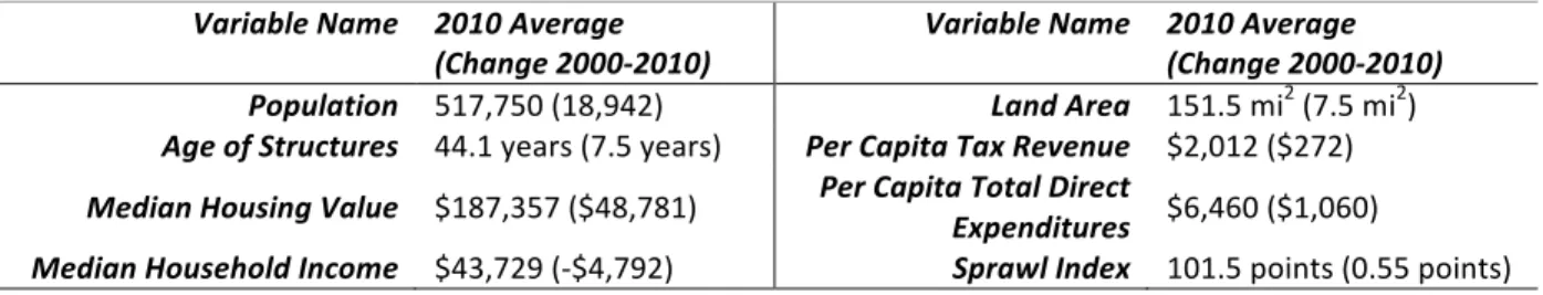
ONFOUNDINGF
ACTORSMany confounding factors could contribute to the relationship between sprawl and
municipal finances (Table 2). These include population growth, the age of the city and
infrastructure, house values, income, tax revenues, and the supply of land. Considering this,
several variables are included to control for these confounding factors, including population
change, change in the median age of structures, change in the median house value for all
owner-occupied units, change in median household income, difference in tax revenues, and change in
the total land area of the city. These data have been collected from the Lincoln Institute’s FiSC
database, the 2000 U.S. decennial census, and the American Community Survey 3-year estimates
(2008-2010). By analyzing the differences over time, inherent differences between cities will be
WELCH 19 accounted for, such as regional variations.
The data on sprawl is calculated at the geography of urbanized area, while the financial data is
calculated at the municipal level. The analysis is still appropriate, despite this misalignment in
geographies, as the overall sprawl/compactness measure for the urbanized area is representative
of the primary central city. Due to the fact that some urbanized areas encompass multiple cities
(consider the urbanized area around San Francisco that includes Oakland and San Jose), it was
necessary to remove cities from the study that fell into the same urbanized area. After removing
these anomalies, 82 large cities remained in unique urbanized areas that could be analyzed in
this study (see Figure 3).
Variable Name 2010 Average
(Change 2000-2010) Variable Name 2010 Average (Change 2000-2010) Population 517,750 (18,942) Land Area 151.5 mi2 (7.5 mi2)
Age of Structures 44.1 years (7.5 years) Per Capita Tax Revenue $2,012 ($272)
Median Housing Value $187,357 ($48,781) Per Capita Total Direct Expenditures $6,460 ($1,060)
Median Household Income $43,729 (-$4,792) Sprawl Index 101.5 points (0.55 points)
WELCH 20
FIGURE 4. THE 82 SELECTED CITIES INCLUDED IN STUDY.
R
EGRESSIONM
ODELSIn order to test the hypothesis, multivariate regression analyses were used to determine
the correlation between the explanatory variable (sprawl) and different municipal financial
variables (exp), controlling for confounding factors, represented by the following equation:
∆"#$ = & + () *$+,-. 01)1 − *$+,-. 0111 + (0 $3$01)1− $3$ 0111 + (4(,6"01)1− ,6"0111) + (8(ℎ:;,.:" 01)1− ℎ:;,.:"0111) + (<(=>?3@"01)1−
=>?3@"0111) + (A(*=B"01)1− *=B"0111) + (C(D,#+01)1− D,#+0111) + E,
where exp is one of the 23 measures of expenditure, sprawl is the calculated sprawl index
developed by Hamidi and Ewing, pop is the total population, age is the median age of structures,
huvalue is the median house value of owner-occupied units, income is the median household
WELCH 21 assessed tax revenue. Twenty-three separate regression models were used, one for each of the
WELCH 22
V.
R
ESULTSThe scatter plot in Figure 4 presents the relationship between the change in total
municipal expenditures and the change in sprawl/compactness between the years 2000 and
2010. As illustrated by the best-fit line, there appears to be a slightly positive linear relationship
between these two variables, although the statistical significance of this line is low (p = 0.32). It
is important to keep in mind that the higher the value in the Sprawl Index, the less sprawling the
city is. The upper-left quadrant of the scatterplot represents the cities that have become more
sprawling and also have increased their per capita total expenditures. Moving clockwise, the
cities in the upper-right quadrant are those that have become more compact while also seeing
an increase in expenditures. The bottom-right quadrant represents the cities that have become
more compact and have reduced their expenditures. This quadrant is the one most linked with
the hypothesis. The final quadrant, the bottom-left, represents the cities that have become more
sprawling and also reduced per capita total expenditures. While the best-fit line suggests a
slightly positive relationship, it is not statistically significant. As the scatterplot shows, cities exist
in all quadrants, showing that cities exist for every combination of spending and sprawl. It is
possible to become more compact and increase spending, or to become more sprawling and
decrease spending. The following regression models will further explore this relationship, as well
WELCH 23
FIGURE 5. SCATTERPLOT OF RELATIONSHIP BETWEEN SPRAWL INDEX AND PER CAPITA DIRECT EXPENDITURES (2000-2010)
Figure 5 presents the summarized regression results for select expenditure models. Of
the 23 regression models, 10 models were statistically insignificant and inconclusive, with very
low F-stat values (less than 1.68), and therefore not included in the summary. The sprawl index
variable was statistically significant and negative in one of the models, as a predictor of capital
outlay. More specifically, the coefficient of -17.18 signifies that for every one percent increase in
the sprawl/compactness index (the city is becoming less sprawling), per capita capital outlay
decreases by 17%. In all other models, the sprawl index had no statistically significant impact on
WELCH 24 Among the confounding variables, tax revenue was the most consistently significant
variable. In eight of the models (expenditures on total direct, education, highway, police, fire,
housing and community development, interest on debt, and debt outstanding) tax revenue was
significant and positive. Increases in tax revenue were associated with increases in spending.
Median house value for all owner-occupied units was significant and positive in seven of the
models (total direct, transportation, fire protection, housing and community development,
transit, and capital outlay expenditures). Population was significant and negative in four models
WELCH 25 (debt outstanding, interest on debt, housing and community development, and fire protection
expenditures), meaning that as population increases, per capita spending and debt decreases.
The median household income was also significant and negative in four models (fire protection,
interest on debt, transit and debt outstanding). As median household income increases,
expenditures in the four areas decreases. Total land area was significant and negative in two of
the models, transportation expenditures and capital outlay.
The remaining variable, median age of structure (a proxy of the age of the city), was
significant and positive for predicting education expenditures, but significant and negative in the
fire protection and parks and recreation models. This suggests that more aging cities spend more
WELCH 26
VI.
D
ISCUSSIONThe regression models found only one significant relationship between sprawl and
municipal expenditures, as a predictor of capital outlay. In line with what the literature and
theoretical models would suggest, as cities become less sprawling and more compact, their
capital outlay decreases. Capital outlay includes spending on the construction or purchase of any
fixed asset or asset upgrade. This can include the acquisition of property, the construction of
buildings and infrastructure, or the completion of any permanent public works or improvement
projects, such as street improvements. The magnitude of this relationship is important, as well.
For every one point increase in “compactness”, there is a 17% decrease in per capita capital
outlay. This can translate into significant savings when taken across the entire population,
especially considering the cities in this study have a median population of more than 295,000.
The other regression models found no significant relationship, positive or negative,
between sprawl and municipal finances, despite strong suggestions in the literature of a negative
relationship. However, most of the theoretical models that have been developed regarding this
issue focus on the general costs of sprawl compared to traditional development patterns. The
results of this research are not able to completely contradict this claim, as this paper only
examined the cost burden to the authority providing the service, such as the municipality, school
district, water board, etc. It is possible that the additional financial costs of sprawl are being
absorbed by another entity, such as developers or consumers. Additional research is needed to
determine if other parties are bearing additional financial burdens as a result of sprawl.
Tax revenue was one factor that did consistently predict spending across categories. Not
WELCH 27 influence tax revenues, including income, political affiliation, and even development. Further
research should be conducted to examine the relationship between development patterns and
tax revenues. It is also important to consider that this paper only examined the actual realized
financial costs (in spending or debt) of sprawl, and none of the environmental or social costs that
have been thoroughly documented in existing literature.
This research found the primary costs of sprawling development patterns to be
embedded in constructing new assets and infrastructure and improving existing infrastructure
(capital outlay). The results suggest that there is no significant difference in the costs of
administering and maintaining existing services between sprawling and compact cities, despite
what existing literature would suggest. However, cities of all kinds are building and acquiring new
assets regularly. Even after controlling for population growth, the age of the city, and total land
area, capital outlay in more sprawling areas is significantly higher. In other words, even as
compact cities build and acquire new assets and infrastructure, it costs significantly less.
These findings emphasize the importance of investing in compactness and accessibility.
While reversing the trend of low-density, poorly planned suburbanization is complex and will
require significant investments, they can be offset by savings in capital outlay over time. Urban
form and infrastructure are very rigid elements of any city. A typical freeway lifespan is in excess
of 50 years. Once a sprawling, poorly connected subdivision is built, it is very difficult to change.
Investments in infrastructure and urban form have the capability to “lock-in” cities for decades,
in terms of physical space, population, livability, carbon emissions, and financial obligations.
WELCH 28 considered. Cities that choose to invest in development that continues the process of urban
sprawl will be forced to live with the increased financial obligations of more costly capital outlay,
in addition to the numerous increased environmental and social costs, decades into the future.
However, cities that choose to invest in compact, accessible development can expect significantly
less capital outlay expenditures for decades to come, in addition to a healthier, more livable
community. At a time when municipal budgets are severely strained, potential savings of any
kind should be seriously considered, especially when the savings offer co-benefits of improved
accessibility, higher social capital, and increased environmental protection.
This research only begins to uncover the extreme complexity of municipal fiscal patterns.
The regression analysis shows that no one factor can explain municipal finances, rather many
variables influence spending, debt, and capital outlay of cities and other authorities responsible
for providing services; this analysis only scratched the surface. Exogenous factors such as natural
disasters, economic influencers, and failing infrastructure certainly play a role in municipal
finances, and may overshadow the costs inflicted by sprawl or compact development.
Furthermore, factors can influence various categories of spending in different, sometimes
opposing, ways. This research also focused broadly on general expenditures, that included the
administrative and daily functioning expenses. However, the one significant variable was capital
outlay – the actual construction or purchase of real assets across all categories – and did not
include any administrative costs. Future research should analyze the impacts of sprawl on
individual categories of capital outlay, such as sewerage, waste management, highways, and
WELCH 29 While this research does strongly support denser, mixed-use, more accessible
development, it does not advocate for any one kind of compact urban form that cities should
design and build. There is no one prescriptive compact urban form that is right for all cities.
Compactness and sustainable urban form looks different everywhere, depending on local context
and citizens’ desires and preferences. However, this research shows that it does matter
significantly to cities’ finances. Urban form and land use patterns have serious financial
WELCH 30
R
EFERENCESBurchell, R. W., Shad, N. A., Listokin, D., Phillips, H., Downs, A., Seskin, S., … Gall, M. (1998). The costs of sprawl--revisited. Transportation research board.
Carruthers, J. I., & Ulfarsson, G. F. (2003). Urban sprawl and the cost of public services. Environment and Planning B: Planning and Design, 30(4), 203–522.
http://doi.org/10.1068/b12847
Cox, W., & Utt, J. (2004). The Costs of Sprawl Reconsidered : What the Data Actually Show, 4999(1770), 20. Retrieved from http://www.heritage.org/research/reports/2004/06/the-costs-of-sprawl-reconsidered-what-the-data-really-show
Ewing, Reid, Pendall, Rolf, and Chen, D. (2000). Measuring Sprawl and Its Impact. Smart Growth America, I, 1–55.
http://www.smartgrowthamerica.org/documents/MeasuringSprawlTechnical.pdf
Frank, J.E. (1989) The costs of alternative development patterns: a review of the literature. Urban Land Institute, Washington, DC.
Glaeser, E. L., & Kahn, M. E. (2004). Chapter 56 Sprawl and urban growth. Handbook of Regional and Urban Economics (Vol. 4). Elsevier Inc. http://doi.org/10.1016/S1574-0080(04)80013-0
Gonter, N. H. (2008, July 18). “Residents fear housing density”. The Republican (Springfield, MA). Accessed via NewsBank, Inc. on February 16, 2017.
Hamidi, S., Ewing, R., Preuss, I., & Dodds, A. (2015). Measuring Sprawl and Its Impacts: An Update. Journal of Planning Education and Research, 35(1), 35–50.
http://doi.org/10.1177/0739456X14565247
Hortas-Rico, M., & Sole-Olle, a. (2010). Does Urban Sprawl Increase the Costs of Providing Local Public Services? Evidence from Spanish Municipalities. Urban Studies, 47(7), 1513–1540.
http://doi.org/10.1177/0042098009353620
Huang, J., Lu, X. X., & Sellers, J. M. (2007). A global comparative analysis of urban form: Applying spatial metrics and remote sensing. Landscape and Urban Planning, 82(4), 184– 197. http://doi.org/10.1016/j.landurbplan.2007.02.010
Kew, B., & Lee, B. D. (2013). Measuring sprawl across the urban rural continuum using an amalgamated sprawl index. Sustainability (Switzerland), 5(5), 1806–1828.
WELCH 31 Laidley, T. (2015). Measuring Sprawl: A New Index, Recent Trends, and Future Research. Urban
Affairs Review, 1–32. http://doi.org/10.1177/1078087414568812
Levenson, E. (2015, March 26). “Homeowners fear high-density zoning”. The Intelligencer (Doylestown, PA). Accessed via NewsBank, Inc. on February 16, 2017.
Lincoln Institute of Land Policy. Fiscally Standardized Cities database.
http://www.lincolninst.edu/subcenters/fiscally-standardized-cities/. Accessed on: September 28, 2016.
Pendall, R. (1999). Do land-use controls cause sprawl? Environment and Planning B: Planning and Design, 26(4), 555–571. http://doi.org/10.1068/b260555
Sholtis, B. (2016, December 17). “Residents fear ‘urban sprawl’ in Hellam Twp.”. The York Record (York, PA). Accessed via NewsBank, Inc. on February 16, 2017.
Slack, E. (2002). Municipal Finance and the Pattern of Urban Growth. Ottawa: C.D.Howe Institute, (160). Retrieved from
http://sfx.scholarsportal.info.ezproxy.library.yorku.ca/york?url_ver=Z39.88-2004&rft_val_fmt=info:ofi/fmt:kev:mtx:journal&genre=article&sid=ProQ:ProQ%3Aabiglob al&atitle=Municipal+Finance+and+the+Pattern+of+Urban+Growth&title=Commentary+-+C.D.+Howe+Insti
WELCH 32