A multi-objective model for the residential waste collection location-routing problem with time windows

(1)

227

A multi-objective model for the residential waste collection

location-routing problem with time windows

Masoud Rabbani

1*

, Neda Manavizadeh

2

, Abtin Boostani

1

, Soroush Aghamohamadi

1

1_{School of Industrial Engineering, College of Engineering, University of Tehran, Tehran, Iran} 2_{Department of Industrial Engineering, KHATAM University, Tehran, Iran}

mrabani@ut.ac.ir, n.manavi@khatam.ac.ir, a_boostani@ut.ac.ir, aghamohamadi.sor@ut.ac.ir

Abstract

This paper presents a novel multi-objective location arc-routing model in order to locate disposal facilities and to design optimal routes of residential waste taking into consideration many complicated real constraints such as a heterogeneous fleet of vehicles, time windows for customers, disposal facilities and the depot, capacities for vehicles and facilities. The first objective is the minimization of transportation costs, including service costs and fuel costs of vehicles. The second one minimizes total number of utilized vehicles. And finally, the third objective function is considered for minimizing total number of established disposal centers. Moreover, to come closer to reality the service time, amount of demands, capacities and cost parameters are considered as fuzzy ones. To solve the proposed model, a credibility-based fuzzy mathematical model and its interactive solution method with three recent approaches, are used and the results are compared with each other.

Keywords: Waste collection problem, multi-objective optimization, time

windows, interactive fuzzy programming, chance constraint programming

1-Introduction

A waste collection system generally involves the collection of waste residues and transportation of them to disposal facilities. This important service is getting more and more attention from many researchers because of its impact on the public interest in the growth of the environment and the population, especially in urban areas. Because the operational cost of this service is very high, researchers are attempting to improve vehicle routing of waste collection in order to reduce the cost, finding the most appropriate location of disposal facilities and the collection site of waste containers while minimizing the number of vehicles used. There are three classes of waste collection problems: residential (or household), commercial and industrial (or rollon-rolloff) (Golden et al., 2002).

In this paper, the Residential Waste Collection Location Arc-Routing Problem (RWCLARP) is developed on a mixed graph. A central depot with heterogeneous fleet of vehicles with limited capacity on the problem network is available. In proposed problem, the household wastes located on the arcs of the network (clients) are collected by available vehicles and transferred to the waste disposal centers. The number of established disposal centers, also the number of different used vehicles, will be determined so that the total costs of traveling and servicing, costs of utilizing vehicles and establishing disposal centers considering defined constraints are minimized.

The considered constraints are as follows; arcs with demand (required arcs) must be fully satisfied i.e. generated wastes that are ready to collect in the streets (arcs), must be fully collected. During each trip, the total collected loads must not exceed that vehicle capacity; also, the total amount of loads (wastes) delivered by different vehicles to any of the disposal centers must not to be greater than the capacity of that center. We define a minimum required demand for establishing disposal centers. *Corresponding author

Vol. 12, No. 4, pp. 227-241 Autumn (November) 2019

(2)

228

Most of researches ignore the role of timing in a supply chain system; however, in real word, timing plays an important role in different parts of a supply chain system including production and delivery parts (Rabbani et al., 2019; Manavizadeh et al., 2019). Delivery and Lack of timely collection of garbage in many cities of developing countries will lead to an unhealthy environment and prevalence of many diseases and many people suffering from those diseases. Thus, for our problem, time windows are considered. Time windows for costumers (required arcs) mean that each customer must be serviced in defined timeframe of the customer besides for central depot and disposal facilities, time windows represent that the vehicles are allowed to visit centers only when they are open.

In many real situations, the input parameters of supply chains and residential garbage collection problem, such as service times, demands, service costs and etc. can be uncertain (Aghamohammadi-Bosjin et al., 2019; Sabouhi and Jabalameli, 2019). For example, sometimes it is possible that the service time of a vehicle to be variable and non-constant, because of changing in traffic density of a certain arc (street) or possibility of occurring an accident and unforeseen repair for a vehicle on the arc. Similarly, the amount of the waste produced in the required arcs (arc's demand) can be different from primary assumed demand. So in this paper, we'll be able to reach the more realistic residential waste collection problem, by considering the uncertainties for service times for required arcs; demands of customers; disposal centers’ capacities and fixed opening costs; vehicles' capacities and fixed utilizing costs and service costs.

The remainder of this paper is organized as follows. The related literature is reviewed in section 2. The definition and mathematical formulation of the proposed problem are described in section 3. A solution methodology is presented in section 4. Finally, the computational results and conclusions are provided in sections 5 and 6 respectively.

2-Literature review

Waste collection problems were introduced as one of the applications of vehicle routing problem (VRP) by Golden et al. (2002). Tung and Pinnoi (2000) developed mathematical models for the residential waste collection problem also they presented a heuristic method and applied that to real practical problems. Miranda et al. (2015) introduced a novel modeling to take into account different aspects of household waste management system. their model includes a decision-making system to determine the waste collection sites, scheduling program for selected sites and assignment of best routs to each vehicle to minimize the costs. They assumed three different scenarios to deal with the problem, in two scenarios the main area divided to sub areas while in the last one they solved the problem on a unique area. Hoang son and Louati (2016 ( proposed a municipal solid waste collection problem including multiple transfer stations, gather sites and inhomogeneous vehicles in a specific period of time affected by waiting time and traffic stops. Rabbani et al. (2018) introduced a hazardous waste location routing problem with different types of collection vehicles and a distance constraint. The feature of this study is about incompatibility between some kinds of wastes that makes the problem more realistic and complicated. Asefi, Lim and Maghrebi (2015) also studied a municipal solid waste dealing with varied types of wastes for transportation and disposal process. Farrokhi-Asl et al. (2017) assumed a waste collection system as a reverse logistic system comprised of depots and disposal centers and formulated the problem as a bi objective problem aimed to optimize social and economic objectives and proved that NSGA-II achieves better results rather than MOPSO algorithm. Huang and Lin (2015) used a set covering problem to deal with location assignment of a municipal waste collection location routing problem by considering time constraint and split delivery which shows there is different ways to deal with a location routing problem and depends of researcher's point of view. Mourao and Almeida (2000) utilized a capacitated arc routing problem to model the problem of residential waste collection in a quarter of Lisbon, Portugal. Bautista et al. (2008) modeled problem of urban waste collection as an arc routing problem.

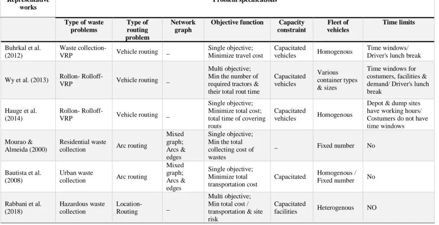
Reviewing the literature related to the waste location-routing problem, there are some works investigating location-routing problem about industrial hazardous wastes/ materials (hazmat). Some of main contributions are summarized in Table 1 which shows only two papers have modeled the waste collection problem as an arc routing one. Hence, location arc-routing approach is proposed for the first time to deal with waste collection problem in this study.

(3)

229

3-Problem definition and formulation

In this paper, we define a new residential waste collection location arc-routing problem (RWCLARP). Three objective functions are considered to the proposed problem. The first goal of our RWCLARP is the minimization of transportation costs, including service costs (removal, transportation and discharge costs of wastes) and fuel costs of vehicles (costs of passing arcs without picking wastes up). The second one minimizes total number of utilized vehicles. And finally, the third objective function is considered for minimizing total number of established disposal centers. The expressed objective functions must be optimized considering following constraints; required arcs must be fully met. During each trip, the total collected garbage must not exceed the vehicle capacity; also, the total amount of wastes delivered by different vehicles to any of the disposal centers must not to be greater than the capacity of the center.

It is noteworthy that because of the conflicting nature of assumed objective functions, the proposed problem considered as a multi-objective model. In this study, for each of required arc (customer) also for waste disposal centers and the central depot, time windows are assigned.

To deal with the issue of uncertainty in developed problem, we use a hybrid credibility-based chance constrained programming model was proposed by Pishvaee et al. (2012). The uncertain parameters are considered as independent trapezoidal fuzzy numbers. The main advantages of the hybrid credibility - based chance constrained programming method are stated as follows (Pishvaee et al., 2012):

 Generally, the credibility-based chance constrained programming is a computationally efficient fuzzy mathematical programming approach that relies on strong mathematical concepts and can support different kinds of fuzzy numbers such as triangular and trapezoidal forms as well as enabling the decision maker to satisfy some chance constraints in at least some given confidence levels.

 Despite the possibility measure that has no self-duality property, the credibility measure is a self-dual measure.

 this hybrid approach does not increase the number of constraints and do not need additional information for objective function such as confidence level or the ideal solution, and also is benefited from advantages of the chance constrained programming approach while dealing with the model constraints.

We used the expected value to model the objective functions and the chance constrained programming method to model the constraints with uncertain parameters.

(4)

230

Table 1. Summary of main contributions in waste collection problem

Representative works

Problem specifications

Type of waste problems

Type of routing problem

Network graph

Objective function Capacity constraint

Fleet of vehicles

Time limits

Buhrkal et al. (2012)

Waste collection-

VRP Vehicle routing _

Single objective; Minimize travel cost

Capacitated

vehicles Homogenous

Time windows/ Driver's lunch break

Wy et al. (2013) Rollon- Rolloff-

Multi objective; Min the number of required tractors & their total rout time

Capacitated vehicles

Various container types & sizes

Time windows for costumers, facilities & demand/ Driver's lunch break

Hauge et al. (2014)

Rollon- Rolloff-

Single objective; Minimize total cost; total time of covering routs

Capacitated

vehicles Homogenous

Depot & dump sites have working hours/ Costumers do not have time windows

Mourao & Almeida (2000)

Residential waste

collection Arc routing

Mixed graph; Arcs & edges

Single objective; Min the total collecting cost of wastes

_ Fixed number No

Bautista et al. (2008)

Urban waste

collection Arc routing

Mixed graph; Arcs & edges

Single objective; Minimize total transportation cost

Capacitated Homogenous / Fixed number No

Rabbani et al. (2018)

Hazardous waste collection

Location-

Routing _

Multi objective; Min total cost / transportation & site risk

Capacitated

(5)

231

3-1- Notation

Notations of the developed model are as follows:

Sets:

𝑉 Set of all network nodes

𝐾 Set of the vehicles at the central depot

𝐸 Set of network edges; ([𝑖, 𝑗])

𝐸𝑅 Set of edges with non-negative demand (required edges) 𝐴 Set of network arcs; (𝑖, 𝑗)

𝐴𝑅 Set of arcs with non-negative demand (required arcs)

𝐷 Set of potential sites for the construction of waste disposal centers

Parameters:

𝑐𝑖𝑗𝑘 Cost of servicing to arc (𝑖. 𝑗) by vehicle 𝑘

𝑐𝑖𝑗𝑘́ Passing cost of vehicle 𝑘 from arc (𝑖. 𝑗) without servicing (fuel cost) 𝑞𝑖𝑗 Demand of arc 𝑖 − 𝑗 (amount of generated waste on arc (𝑖. 𝑗)) 𝑓𝑣𝑘 Fixed cost of utilizing vehicle 𝑘

𝑓𝑑𝑖 Fixed cost of establishing garbage disposal center 𝑖

𝑣𝑐𝑘 Capacity of vehicle 𝑘 (Maximum permissible load capacity) 𝑑𝑐𝑖 Capacity of garbage disposal center𝑖

𝑑𝑐𝑖𝑚 The minimum amount of required waste for the establishment of disposal center 𝑖 𝑡𝑖𝑗𝑘 Passing time of vehicle 𝑘 from arc (𝑖. 𝑗)

𝑠𝑖𝑗𝑘 Servicing time of vehicle 𝑘 to arc (𝑖. 𝑗)

𝑀 A very large numberto be considered equal to the sum of all demands (𝑀 = ∑(𝑖.𝑗)𝜖𝐴𝑅𝑞𝑖𝑗).

𝑎𝑖𝑗 Earliest time to begin servicing arc (𝑖. 𝑗) 𝑏𝑖𝑗 Latest time to begin servicing arc (𝑖. 𝑗)

𝑔𝑗 Earliest time to enter the disposal center 𝑗 (when the center opens) ℎ𝑗 Latest time to enter the disposal center 𝑗 (when the center will be closed) 𝑚 Earliest time for vehicle transit from/to central depot (when the depot opens)

𝑛 Latest time for vehicle transit from/to central depot (when the depot will be closed)

Variables:

𝑙𝑖𝑗𝑘 is a binary variable;equal to 1 if vehicle 𝑘 serves [𝑖. 𝑗] from 𝑖 to 𝑗 and equal to 0, otherwise

𝑙𝑖𝑗𝑘́ is a binary variable; equal to 1 if vehicle 𝑘 passes arc 𝑖 − 𝑗 without servicing and equal to 0, otherwise

𝑣𝑘 is a binary variable; equal to 1 if vehicle 𝑘be used and equal to 0, otherwise 𝑤𝑖𝑗𝑘 The total amount of loads (garbage) that vehicle 𝑘 has collected while passing arc

𝑖 − 𝑗

𝑑𝑖 is a binary variable; equal to 1 if a waste disposal centeris established at the node of 𝑖 ∈ 𝐷and equal to 0, otherwise

𝑑𝑖𝑠𝑖 The amount of collected waste at the node of 𝑖 ∈ 𝐷 𝑢𝑖𝑗𝑘 Arrival time of vehicle 𝑘 to the beginning of the arc (𝑖. 𝑗) 𝑢𝑖𝑗𝑘́ Arrival time of vehicle 𝑘 to the end of the arc (𝑖. 𝑗)

Besides, assumed time windows for costumers, disposal centers and central depot are as follows:

(6)

232

[𝑔𝑗. ℎ𝑗] Allowed timeframe for visiting waste disposal center 𝑗 [𝑚. 𝑛] Allowed timeframe for visiting central depot

3-2- Mathematical model

The formulation of considered credibility-based fuzzy mathematical programming is as follows. 𝑀𝑖𝑛 𝐸[𝑓1] = ∑ ∑ 𝐸[𝑐̃𝑖𝑗𝑘]. 𝐸[𝑞̃𝑖𝑗]. 𝑙𝑖𝑗𝑘

(𝑖.𝑗)∈𝐴𝑅

𝑘∈𝐾

+ ∑ ∑ 𝑐𝑖𝑗𝑘́ . 𝑙𝑖𝑗𝑘́ (𝑖.𝑗)∈𝐴 𝑘∈𝐾

(1)

𝑀𝑖𝑛 𝐸[𝑓2] = ∑ 𝐸[𝑓𝑣̃𝑘]. 𝑣𝑘 𝑘∈𝐾 (2)

𝑀𝑖𝑛 𝐸[𝑓3] = ∑ 𝐸[𝑓𝑑̃𝑖]. 𝑑𝑖 𝑖∈𝐷 (3)

Subject to: ∑ 𝑙𝑖𝑗𝑘 𝑖 = ∑ 𝑙𝑗𝑖́𝑘 𝑖́ ∀𝑗 ∈ 𝑉. ∀𝑘 ∈ 𝐾. 𝑗 ≠ 1. (𝑖. 𝑖́ ≠ 𝑗) (4)

∑ 𝑙𝑖𝑗𝑘́ 𝑖 = ∑ 𝑙𝑗𝑖́𝑘́ 𝑖́ ∀𝑗 ∈ 𝑉. ∀𝑘 ∈ 𝐾. 𝑗 ≠ 1. (𝑖. 𝑖́ ≠ 𝑗) (5)

∑ 𝑙1𝑗𝑘 𝑗 = ∑ 𝑙𝑖1𝑘≤ 1 𝑖 ∀𝑘 ∈ 𝐾 (6)

∑ 𝑙1𝑗𝑘́ 𝑗 = ∑ 𝑙𝑖1𝑘́ ≤ 1 𝑖 ∀𝑘 ∈ 𝐾 (7)

𝑙𝑖𝑗𝑘≤ 𝑣𝑘 ∀𝑘 ∈ 𝐾. ∀(𝑖. 𝑗) ∈ 𝐴 (8)

𝑙𝑖𝑗𝑘́ ≤ 𝑣𝑘 ∀𝑘 ∈ 𝐾. ∀(𝑖. 𝑗) ∈ 𝐴 (9)

∑ 𝑙𝑖𝑗𝑘= 1 𝑘 ∀(𝑖. 𝑗) ∈ 𝐴𝑅. 𝑖 ≠ 𝑗 (10)

𝑤𝑖1𝑘= 0 ∀𝑖 ∈ 𝑉. ∀𝑘 ∈ 𝐾 (11)

𝑤1𝑗𝑘 = 0 ∀𝑗 ∈ 𝑉. ∀𝑘 ∈ 𝐾 (12)

𝐶𝑟{𝑣𝑐̃𝑘(𝑙𝑖𝑗𝑘− 1) ≤ 𝑤𝑖𝑗𝑘− 𝑤𝑡𝑖𝑘− 𝑞̃𝑖𝑗} ≥ 𝛼𝑘 ∀{(𝑖. 𝑗). (𝑡. 𝑖)}; (𝑖. 𝑗) ≠ (𝑡. 𝑖). ∀𝑘 ∈ 𝐾 (13)

𝐶𝑟{𝑞̃𝑖𝑗 ≤ 𝑤𝑖𝑗𝑘} ≥ 𝛽𝑖𝑗 ∀(𝑖. 𝑗) ∈ 𝐴. ∀𝑘 ∈ 𝐾 (14)

𝐶𝑟{𝑣𝑐̃𝑘≥ 𝑤𝑖𝑗𝑘} ≥ 𝛼𝑘 ∀(𝑖. 𝑗) ∈ 𝐴. ∀𝑘 ∈ 𝐾 (15)

∑ ∑ 𝑤𝑖𝑗𝑘 𝑘 𝑖 = 𝑑𝑖𝑠𝑗 ∀𝑗 ∈ 𝐷 (16)

𝐶𝑟 { ∑ 𝑞̃𝑖𝑗 (𝑖.𝑗)𝜖𝐴𝑅 ≤ ∑ 𝑑𝑖𝑠𝑡 𝑡∈𝐷 } ≥ 𝛽_𝑖𝑗 (17)

(7)

233 𝐶𝑟 { ∑ 𝑞̃𝑖𝑗

(𝑖.𝑗)𝜖𝐴_𝑅

≥ ∑ 𝑑𝑖𝑠𝑡 𝑡∈𝐷

} ≥ 𝛽𝑖𝑗 (18)

𝐶𝑟{𝑑𝑐̃𝑖. 𝑑𝑖≥ 𝑑𝑖𝑠𝑖} ≥ 𝛾𝑖 ∀𝑖 ∈ 𝐷 (19)

𝑑𝑖𝑠𝑖≥ 𝑑𝑐𝑖𝑚. 𝑑𝑖 ∀𝑖 ∈ 𝐷 (20)

𝑎𝑖𝑗 ≤ 𝑢𝑖𝑗𝑘≤ 𝑏𝑖𝑗 ∀(𝑖. 𝑗) ∈ 𝐴𝑅. ∀𝑘 ∈ 𝐾 (21)

𝐶𝑟{𝑠̃𝑖𝑗𝑘≤ 𝑢𝑗𝑡𝑘− 𝑢𝑖𝑗𝑘− 𝑡𝑖𝑗𝑘+ (1 − 𝑙𝑖𝑗𝑘). 𝑀} ≥ 𝜃𝑖𝑗𝑘 ∀(𝑖. 𝑗) ∈ 𝐴𝑅. ∀𝑡 ∈ 𝑉. ∀𝑘 ∈ 𝐾 (22)

𝑔𝑗≤ 𝑢𝑖𝑗𝑘́ ≤ ℎ𝑗 ∀𝑘 ∈ 𝐾. ∀𝑗 ∈ 𝐷 (23)

𝑚 ≤ 𝑢1𝑗𝑘≤ 𝑛 ∀𝑗 ∈ 𝑉. ∀𝑘 ∈ 𝐾 (24)

𝑚 ≤ 𝑢𝑖1𝑘́ ≤ 𝑛 ∀𝑖 ∈ 𝑉. ∀𝑘 ∈ 𝐾 (25)

𝐶𝑟{𝑠̃𝑖𝑗𝑘. 𝑙𝑖𝑗𝑘≥ 𝑢́𝑖𝑗𝑘− 𝑢𝑖𝑗𝑘− 𝑡𝑖𝑗𝑘} ≥ 𝜃𝑖𝑗𝑘 ∀(𝑖. 𝑗) ∈ 𝐴𝑅. ∀𝑡 ∈ 𝑉. ∀𝑘 ∈ 𝐾 (26)

𝐶𝑟{𝑠̃𝑖𝑗𝑘. 𝑙𝑖𝑗𝑘≤ 𝑢́𝑖𝑗𝑘− 𝑢𝑖𝑗𝑘− 𝑡𝑖𝑗𝑘} ≥ 𝜃𝑖𝑗𝑘 ∀(𝑖. 𝑗) ∈ 𝐴𝑅. ∀𝑡 ∈ 𝑉. ∀𝑘 ∈ 𝐾 (27)

𝑙𝑖𝑗𝑘 . 𝑙𝑖𝑗𝑘́ . 𝑣𝑘. 𝑑𝑡∈ {0.1} ∀(𝑖. 𝑗) ∈ 𝐴. ∀𝑘 ∈ 𝐾. ∀𝑡 ∈ 𝐷 (28)

𝑤𝑖𝑗𝑘≥ 0 ∀(𝑖. 𝑗) ∈ 𝐴. ∀𝑘 ∈ 𝐾 (29)

𝑑𝑖𝑠𝑖≥ 0 ∀𝑖 ∈ 𝐷 (30)

𝑢𝑖𝑗𝑘≥ 0 ∀(𝑖. 𝑗) ∈ 𝐴. ∀𝑘 ∈ 𝐾 (31)

𝑢𝑖𝑗𝑘́ ≥ 0 ∀(𝑖. 𝑗) ∈ 𝐴. ∀𝑘 ∈ 𝐾 (32)

Equations (1) to (3) are the expected value of three objection functions which expressed before. Set of constraints (4) and (5) guarantee the continuity of tour. Constraints (6) and (7) indicated that if a vehicle is used, it can only go in one direction starting from the depot and service to required arcs accordingly and by the end of its tour, it must return to the central depot. Constraints (8) and (9) guarantee that a vehicle is traveling along arc 𝑖 − 𝑗, only if it is used from the central depot. Constraints on relation (10) ensure that each required arc must be served with one vehicle. Constraints (11) and (12) indicate that each used vehicle must be empty while starting a route from the depot and when it returns to the central depot at the end of the route.

Constraints number (13) to (15) is fuzzy sub-tour elimination constraints which are introduced by Kara et al. (2004) for the capacitated vehicle routing problems. Constraints (16) represent the material balance limitations between the total collected wastes by different vehicles that have been transported to each disposal center and the total delivered loads to that center. Constraints (17) and (18) are the material flow balance limitations between the required arcs and the waste disposal centers. Constraints (19) ensure that the capacity of disposal centers must be respected and not violated. Constraints (20) determine the minimum amount of required waste to establish a disposal center. Constraints number (21) and (22) consider the time windows for servicing the required arcs. Constraints (23) determine the time windows for visiting the disposal centers, besides constraints number (24) and (25) are for considering time windows of outing from the depot and entering to it, respectively. Constraints (26) and (27) denote the relation between the "arrival time of vehicles to the beginning of the arc" and the "arrival time of vehicles to the end of the arc". Remaining constraints define the variables nature.

(8)

234

Then, we transform the presented model to the crisp equivalent MILP one considering the expected value of trapezoidal fuzzy numbers and using (33) and (34) relations (proved by Zhu and Zhang (2009));

𝐶𝑟{𝜉̃ ≤ 𝑘} ≥ 𝛼 ⇔ 𝑘 ≥ (2 − 2𝛼)𝜉₍₃₎+ (2𝛼 − 1)𝜉₍₄₎. (33) 𝐶𝑟{𝜉̃ ≤ 𝑘} ≥ 𝛼 ⇔ 𝑘 ≥ (2 − 2𝛼)𝜉(3)+ (2𝛼 − 1)𝜉(4). (34)

Thus, relations (1) to (3) are substituted by relations (35) to (37) and constraints number (13), (14), (15), (17), (18), (19), (22), (26) and (27) are substituted by constraints (38) to (46) respectively. 𝑀𝑖𝑛 𝐸[𝑓1] = ∑ ∑ (

𝑐𝑖𝑗𝑘(1)+ 𝑐𝑖𝑗𝑘(2)+ 𝑐𝑖𝑗𝑘(3)+ 𝑐𝑖𝑗𝑘(4)

4 )(

𝑞𝑖𝑗(1)+ 𝑞𝑖𝑗(2)+ 𝑞𝑖𝑗(3)+ 𝑞𝑖𝑗(4)

4 )𝑙𝑖𝑗𝑘

(𝑖.𝑗)∈𝐴𝑅

𝑘∈𝐾

+ ∑ ∑ 𝑐𝑖𝑗𝑘́ . 𝑙𝑖𝑗𝑘́ (𝑖.𝑗)∈𝐴 𝑘∈𝐾

(35)

𝑀𝑖𝑛 𝐸[𝑓2] = ∑(

𝑓𝑣𝑘(1)+ 𝑓𝑣𝑘(2)+ 𝑓𝑣𝑘(3)+ 𝑓𝑣𝑘(4)

4 )𝑣𝑘

𝑘∈𝐾

(36)

𝑀𝑖𝑛 𝐸[𝑓3] = ∑(

𝑓𝑑𝑖(1)+ 𝑓𝑑𝑖(2)+ 𝑓𝑑𝑖(3)+ 𝑓𝑑𝑖(4)

4 )𝑑𝑖

𝑖∈𝐷

(37)

𝑤𝑖𝑗𝑘− 𝑤𝑡𝑖𝑘≥ (𝑙𝑖𝑗𝑘− 1)[(2 − 2𝛼𝑘)𝑣𝑐𝑘(3)+ (2𝛼𝑘− 1)𝑣𝑐𝑘(4)] + [(2 − 2𝛽𝑖𝑗)𝑞𝑖𝑗(3)

+ (2𝛽𝑖𝑗− 1)𝑞𝑖𝑗(4)] ∀{(𝑖. 𝑗). (𝑡. 𝑖)}; (𝑖. 𝑗) ≠ (𝑡. 𝑖). ∀𝑘 ∈ 𝐾 (38)

𝑤𝑖𝑗𝑘≥ (2 − 2𝛽𝑖𝑗)𝑞𝑖𝑗(3)+ (2𝛽𝑖𝑗− 1)𝑞𝑖𝑗(4) ∀(𝑖. 𝑗) ∈ 𝐴. ∀𝑘 ∈ 𝐾 (39)

𝑤𝑖𝑗𝑘≤ (2𝛼𝑘− 1)𝑣𝑐𝑘(1)+ (2 − 2𝛼𝑘)𝑣𝑐𝑘(2) ∀(𝑖. 𝑗) ∈ 𝐴. ∀𝑘 ∈ 𝐾 (40)

∑ 𝑑𝑖𝑠_𝑡

𝑡∈𝐷

≥ ∑ [

(𝑖.𝑗)𝜖𝐴𝑅

(2 − 2𝛽_𝑖𝑗)𝑞_𝑖𝑗(3)+ (2𝛽𝑖𝑗− 1)𝑞𝑖𝑗(4)] (41)

∑ 𝑑𝑖𝑠𝑡 𝑡∈𝐷

≤ ∑ [

(𝑖.𝑗)𝜖𝐴𝑅

(2𝛽𝑖𝑗− 1)𝑞𝑖𝑗(1)+ (2 − 2𝛽𝑖𝑗)𝑞𝑖𝑗(2)] (42)

𝑑𝑖𝑠𝑖≤ 𝑑𝑖. [(2𝛾𝑖− 1)𝑑𝑐𝑖(1)+ (2 − 2𝛾𝑖)𝑑𝑐𝑖(2)] ∀𝑖 ∈ 𝐷 (43)

𝑢𝑗𝑡𝑘− 𝑢𝑖𝑗𝑘− 𝑡𝑖𝑗𝑘+ (1 − 𝑙𝑖𝑗𝑘). 𝑀 ≥ (2 − 2𝜃𝑖𝑗𝑘)𝑠𝑖𝑗𝑘(3)+ (2𝜃𝑖𝑗𝑘− 1)𝑠𝑖𝑗𝑘(4) ∀(𝑖. 𝑗) ∈ 𝐴𝑅. ∀𝑡 ∈ 𝑉. ∀𝑘

∈ 𝐾 (44)

4-The solution methodology

The above-mentioned crisp equivalent model is a multi-objective parametric mixed integer linear programming (MOPMILP) model. We apply a fuzzy interactive method to solve that. Using fuzzy interactive method, allows us to adjust the confidence level of each objective function according to the preferences of decision makers.

It should be noted that in this paper in order to convert the multi-objective model to an equivalent single objective one in the applied interactive method, we have used three different approaches including the TH aggregation function method developed by Torabi & Hassini (2008); SO aggregation function approach proposed by Selim and Ozkarahan (2008); and, fuzzy goal programming approach presented by Ghodratnama et al. (2013) and then compared their results.

4-1- Proposed interactive fuzzy programming solution method

(9)

235

Step 1: Determine proper trapezoidal membership functions for the uncertain parameters and formulate the MOPMILP model for the considered multi-objective RWCLARP-TW.

Step 2: Transform three fuzzy objective functions into their crisp ones using the expected value of uncertain parameters.

Step 3: Determine the minimum acceptable satisfaction level for each fuzzy constraint, i.e.,

𝛼𝑘; 𝛽𝑖𝑗; 𝛾𝑖; 𝜃𝑖𝑗𝑘, convert the fuzzy constraints into their equivalent crisp ones using equations. (33) and (34) and develop the equivalent auxiliary crisp MOPMILP model.

Step 4: Calculate the positive ideal solution (PIS) and negative ideal solution (NIS) for each objective function of proposed problem.

Step 5: Determine a linear membership function for each objective function using the following

relations: 𝜇1(𝑥) = {

1 𝑖𝑓 𝑓1< 𝑓1𝑃𝐼𝑆 𝑓1𝑁𝐼𝑆−𝑓1

𝑓₁𝑁𝐼𝑆_−𝑓 1𝑃𝐼𝑆

𝑖𝑓 𝑓1𝑃𝐼𝑆≤ 𝑓1≤ 0 𝑖𝑓 𝑓1> 𝑓1𝑁𝐼𝑆

𝑓1𝑁𝐼𝑆

𝜇2(𝑥) = {

1 𝑖𝑓 𝑓2< 𝑓2𝑃𝐼𝑆 𝑓2𝑁𝐼𝑆− 𝑓2

𝑓₂𝑁𝐼𝑆_{− 𝑓} 2𝑃𝐼𝑆

𝑖𝑓 𝑓₂𝑃𝐼𝑆_{≤ 𝑓} 2≤ 0 𝑖𝑓 𝑓2> 𝑓2𝑁𝐼𝑆

𝑓2𝑁𝐼𝑆

𝜇3(𝑥) = {

1 𝑖𝑓 𝑓3< 𝑓3𝑃𝐼𝑆 𝑓₃𝑁𝐼𝑆_{− 𝑓}

3 𝑓3𝑁𝐼𝑆− 𝑓3𝑃𝐼𝑆

𝑖𝑓 𝑓3𝑃𝐼𝑆 ≤ 𝑓3≤ 0 𝑖𝑓 𝑓3> 𝑓3𝑁𝐼𝑆

𝑓3𝑁𝐼𝑆

Where 𝜇ℎ(𝑥) is the confidence level of ℎ𝑡ℎ objective function when 𝑥 is the given solution vector.

Step 6: Transform the corresponding crisp MOPMILP model into a single-objective one using the

TH and SO aggregation function.

Step 7: Determine the value of the coefficient of compensation (𝜑) and the relative importance of the fuzzy objectives (𝜔ℎ), then solve the resulting single-objective crisp model. If the obtained solution convinces decision maker, then stop and consider the current solution as the optimal decision; otherwise, change the required parameters such as 𝛼𝑘. 𝛽𝑖𝑗. 𝛾𝑖. 𝜃𝑖𝑗𝑘, 𝜔ℎ and 𝜑 based on the new preferences of the decision maker and go to the step 3.

Notice: For Fuzzy goal programming approach, steps of the proposed algorithm are as follows:

Steps 1-5: As stated before.

Step 6: Formulate the corresponding crisp RWCLARP-TW goal programming model as follows:

max ∑ 𝜌ℎ ℎ𝜏ℎ 𝑠. 𝑡. 𝑥 ∈ 𝐹(𝑥).

𝜏 ∈ [0.1]

Where 𝜌ℎ represents the significance weight factor of theℎ𝑡ℎobjective function which is suggested by the decision maker such that ∑ 𝜌ℎ ℎ= 1.

Step 7: Solve the presented model in step 6. Considering the values of objective function (𝜏ℎ) and 𝑓_ℎ𝑃𝐼𝑆_{, solve the following formulation to obtain the new}_𝑓

ℎ𝑃𝐼𝑆 (𝑓ℎ𝑛𝑒𝑤) or the new 𝜏 (𝜏𝑛𝑒𝑤). max ∑ 𝜌ℎ

ℎ 𝜏ℎ 𝑠. 𝑡. 𝑓_ℎ𝑛𝑒𝑤 _{≤ 𝑓}

ℎ𝑃𝐼𝑆 𝑜𝑟 (𝜏𝑛𝑒𝑤 ≥ 𝜏) ℎ = 1.2.3 𝑥 ∈ 𝐹(𝑥).

𝜏 ∈ [0.1]

(10)

236

Step 8: Solve the presented model in step 7. Considering the obtained values of 𝑓ℎ𝑛𝑒𝑤 and adding the 𝑓_ℎ𝑛𝑒𝑤 ≤ 𝑓_ℎ𝑃𝐼𝑆 𝑜𝑟 (𝜏𝑛𝑒𝑤_{≥ 𝜏)}_{constraint for each}_ℎ_{, calculate different}_{satisfaction levels}₍_𝜏

ℎ).

Step 9: Choose the best values of 𝜏 and 𝑓_ℎ𝑃𝐼𝑆 based on the decision maker's opinion.

5-Computational experiments

To show that the proposed credibility-based fuzzy mathematical model and its interactive solution method are useful for the developed RWCLARP-TW, a real case study for one of Tehran municipality zones is provided here.

In the considered area, there is a network with 8 intersections and 10 required arcs. Three kinds of vehicles are located in the depot. It is possible to establish garbage disposal centers at the intersections number 3, 5 and 7. Open hours of the depot and disposal centers are between 8 pm and 6 am, also required customers could be visited and served between 9 pm and 5 am.

To determine the four prominent values used to specify the corresponding trapezoidal fuzzy numbers, the existing data and knowledge of experienced experts in the related field are utilized. So, data about the amount of generated garbage for required arcs are given in table 2.

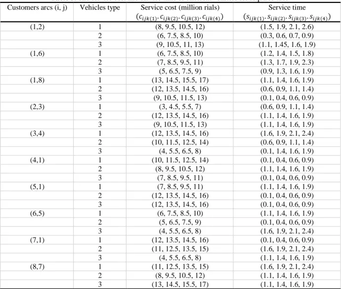
Similarly, for 3 different kinds of vehicles, the service cost and service time of each required arc are represented in Table 3. All monetary data are presented in the Iranian currency (Rial), also time data are presented in hours (hrs).

The fixed cost and capacity data for different vehicles and for disposal centers in any potential location are reported in tables 4 and 5, respectively.

To demonstrate the efficiency of the applied credibility-based fuzzy mathematical model and its interactive solution method according to TH approach, we code this model and methodology by GAMS optimization software and run GAMS code for all test problems on a Core2 Duo Processor 2.2 GHz computer with 3 GB RAM. Different feasibility degrees and importance weights of objective functions are considered for numerical examples (see the first and second columns of table 6). Also, in all cases, the compensation coefficient 𝜑 is set to 0.4.

Table 2. The demand of customers (required arcs) Demand (tons) Customer arcs (i, j)

(𝑞𝑖𝑗(1). 𝑞𝑖𝑗(2). 𝑞𝑖𝑗(3). 𝑞𝑖𝑗(4)) 0.07, 0.095, 0.105, 0.125) )

(1,2)

(0.37, 0.395, 0.405, 0.425) (1,6)

(0.37, 0.395, 0.405, 0.425) (1,8)

0.07, 0.095, 0.105, 0.125) )

(2,3)

(0.47, 0.497, 0.505, 0.525) (3,4)

0.07, 0.095, 0.105, 0.125) )

(4,1)

(0.47, 0.497, 0.505, 0.525) (5,1)

(0.17, 0.195, 0.205, 0.225) (6,5)

0.07, 0.095, 0.105, 0.125) )

(7,1)

(0.47, 0.497, 0.505, 0.525) (8,7)

(11)

237

Table 3. The service cost and service time of different vehicles for required arcs Service time

(𝑠𝑖𝑗𝑘(1). 𝑠𝑖𝑗𝑘(2). 𝑠𝑖𝑗𝑘(3). 𝑠𝑖𝑗𝑘(4))

Service cost (million rials)

(𝑐𝑖𝑗𝑘(1). 𝑐𝑖𝑗𝑘(2). 𝑐𝑖𝑗𝑘(3). 𝑐𝑖𝑗𝑘(4))

Vehicles type Customers arcs (i, j)

(1.5, 1.9, 2.1, 2.6) (8, 9.5, 10.5, 12)

1 (1,2)

(0.3, 0.6, 0.7, 0.9) (6, 7.5, 8.5, 10)

2

(1.1, 1.45, 1.6, 1.9) (9, 10.5, 11, 13)

3

(1.2, 1.4, 1.5, 1.8) (6, 7.5, 8.5, 10)

1 (1,6)

(1.3, 1.7, 1.9, 2.3) (7, 8.5, 9.5, 11)

2

(0.9, 1.3, 1.6, 1.9) (5, 6.5, 7.5, 9)

3

(1.1, 1.4, 1.6, 1.9) (13, 14.5, 15.5, 17)

1 (1,8)

(0.6, 0.9, 1.1, 1.4) (12, 13.5, 14.5, 16)

2

(0.1, 0.4, 0.6, 0.9) (9, 10.5, 11.5, 13)

3

(0.6, 0.9, 1.1, 1.4) (3, 4.5, 5.5, 7)

1 (2,3)

(1.1, 1.4, 1.6, 1.9) (12, 13.5, 14.5, 16)

2

(1.1, 1.4, 1.6, 1.9) (9, 10.5, 11.5, 13)

3

(1.6, 1.9, 2.1, 2.4) (12, 13.5, 14.5, 16)

1 (3,4)

(0.6, 0.9, 1.1, 1.4) (10, 11.5, 12.5, 14)

2

(0.1, 1.4, 1.6, 1.9) (4, 5.5, 6.5, 8)

3

(0.1, 0.4, 0.6, 0.9) (10, 11.5, 12.5, 14)

1 (4,1)

(1.1, 1.4, 1.6, 1.9) (8, 9.5, 10.5, 12)

2

(0.1, 0.4, 0.6, 0.9) (7, 8.5, 9.5, 11)

3

(1.1, 1.4, 1.6, 1.9) (7, 8.5, 9.5, 11)

1 (5,1)

(0.1, 0.4, 0.6, 0.9) (12, 13.5, 14.5, 16)

2

(0.1, 0.4, 0.6, 0.9) (12, 13.5, 14.5, 16)

3

(1.1, 1.4, 1.6, 1.9) (6, 7.5, 8.5, 10)

1 (6,5)

(0.1, 0.4, 0.6, 0.9) (5, 6.5, 7.5, 9)

2

(1.6, 1.9, 2.1, 2.4) (4, 5.5, 6.5, 8)

3

(0.1, 0.4, 0.6, 0.9) (12, 13.5, 14.5, 16)

1 (7,1)

(1.6, 1.9, 2.1, 2.4) (11, 12.5, 13.5, 15)

2

(1.1, 1.4, 1.6, 1.9) (4, 5.5, 6.5, 8)

3

(1.6, 1.9, 2.1, 2.4) (11, 12.5, 13.5, 15)

1 (8,7)

(1.1, 1.4, 1.6, 1.9) (8, 9.5, 10.5, 12)

2

(1.1, 1.4, 1.6, 1.9) (13, 14.5, 15.5, 17)

3

Table 4. The fixed cost and capacity data of different vehicles Vehicle capacity (tons)

(𝑣𝑘𝑘(1). 𝑣𝑘𝑘(2). 𝑣𝑘𝑘(3). 𝑣𝑘𝑘(4))

Fixed cost (million rials)

(𝑓𝑣𝑘(1). 𝑓𝑣𝑘(2). 𝑓𝑣𝑘(3). 𝑓𝑣𝑘(4))

Vehicle type

(0.7, 0.9, 1, 1.25) (35, 46, 50, 60)

1

(1.6, 1.95, 2.1, 2.6) (63, 72, 78, 89)

2

(2.5, 3, 3.1, 3.7) (90, 107, 112, 123)

3

Table 5. The fixed cost and capacity data of disposal facilities Capacity (tons)

(𝑑𝑐𝑖(1). 𝑑𝑐𝑖(2). 𝑑𝑐𝑖(3). 𝑑𝑐𝑖(4))

Fixed cost (million rials)

(𝑓𝑑𝑖(1). 𝑓𝑑𝑖(2). 𝑓𝑑𝑖(3). 𝑓𝑑𝑖(4))

Disposal location

(1.7, 1.95, 2, 2.3) (380, 470, 510, 590)

1

(2.2, 2.5, 2.55, 2.9) (540, 590, 605, 650)

2

(2.6, 2.9, 3.1, 3.4) (640, 685, 705, 770)

(12)

238

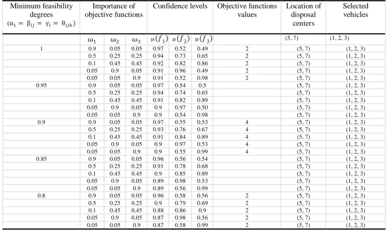
Table 6. The summary of results of TH method

As it can be noticed from table 6, the optimum locations for establishing disposal centers are intersections number 5 and 7. Moreover, when the minimum degree of feasibility is increased the value of the objective function increases, because to cover the demands and reduce the risk of infeasibility in the higher confidence levels, more resources are needed.

Additionally, as the results show, three objective functions divulge the conflicting nature when the importance weight of the first objective function is equal or greater than 0.9 (i.e., ω1= 0.9). On the

other hand, more reliable solutions are gained when 𝜔1varies between 0.5 and 0.05.

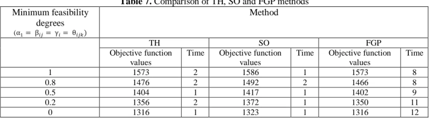
5-1- Comparison of three solution methods

In this section, we compare three concerned solution methods with each other in terms of the objective function values and computational times. To compare these methods, the compensation coefficient values of TH and SO methods are set to 0.4.

The results of FGP method exhibit the minimum objective function values among three considered solution methods; however, the FGP results have obtained in the longest computational time. On the other hand, the SO method requires the least computation time. The TH method produces results that have the objective function values close to the values of FGP method (when Minimum feasibility degrees are equal to 0 and 1, objective function values are the same) but in a much lower computational time (about the computational time of SO method). Thus, the TH method is an advantageous method that offers effective solutions. The comparison results are shown in table 7.

Selected vehicles Location of disposal centers Objective functions values Confidence levels Importance of objective functions Minimum feasibility degrees

(α1= β𝑖𝑗= γ𝑖 = θ𝑖𝑗𝑘)

(1, 2, 3) (5, 7)

(𝑓₃) (𝑓₂) (𝑓₁) ω3

ω2

ω1

(1, 2, 3) (5, 7) 2 0.49 0.52 0.97 0.05 0.05 0.9 1

(1, 2, 3) (5, 7) 2 0.65 0.73 0.94 0.25 0.25 0.5

(1, 2, 3) (5, 7) 2 0.86 0.82 0.92 0.45 0.45 0.1

(1, 2, 3) (5, 7) 2 0.49 0.96 0.91 0.05 0.9 0.05

(1, 2, 3) (5, 7) 2 0.98 0.52 0.91 0.9 0.05 0.05

(1, 2, 3) (5, 7) 0.5 0.54 0.97 0.05 0.05 0.9 0.95

(1, 2, 3) (5, 7) 0.65 0.74 0.94 0.25 0.25 0.5

(1, 2, 3) (5, 7) 0.89 0.82 0.91 0.45 0.45 0.1

(1, 2, 3) (5, 7) 0.50 0.97 0.9 0.05 0.9 0.05

(1, 2, 3) (5, 7) 0.98 0.54 0.9 0.9 0.05 0.05

(1, 2, 3) (5, 7) 4 0.53 0.55 0.97 0.05 0.05 0.9 0.9

(1, 2, 3) (5, 7) 4 0.67 0.76 0.93 0.25 0.25 0.5

(1, 2, 3) (5, 7) 4 0.89 0.84 0.91 0.45 0.45 0.1

(1, 2, 3) (5, 7) 4 0.53 0.97 0.9 0.05 0.9 0.05

(1, 2, 3) (5, 7) 4 0.99 0.55 0.9 0.9 0.05 0.05

(1, 2, 3) (5, 7) 0.54 0.56 0.96 0.05 0.05 0.9 0.85

(1, 2, 3) (5, 7) 0.68 0.78 0.91 0.25 0.25 0.5

(1, 2, 3) (5, 7) 0.89 0.85 0.9 0.45 0.45 0.1

(1, 2, 3) (5, 7) 0.53 0.98 0.89 0.05 0.9 0.05

(1, 2, 3) (5, 7) 0.99 0.56 0.89 0.9 0.05 0.05

(1, 2, 3) (5, 7) 2 0.56 0.58 0.96 0.05 0.05 0.9 0.8

(1, 2, 3) (5, 7) 2 0.69 0.79 0.9 0.25 0.25 0.5

(1, 2, 3) (5, 7) 2 0.9 0.86 0.88 0.45 0.45 0.1

(1, 2, 3) (5, 7) 2 0.56 0.98 0.87 0.05 0.9 0.05

(1, 2, 3) (5, 7) 2 0.99 0.58 0.87 0.9 0.05 0.05

(13)

239

Table 7. Comparison of TH, SO and FGP methods

Method Minimum feasibility

degrees

(α1= β𝑖𝑗= γ𝑖= θ𝑖𝑗𝑘)

FGP SO

TH

Time Objective function

values Time

Objective function values Time

Objective function values

8 1573

1 1586

2 1573

1

8 1466

2 1492

2 1476

0.8

9 1402

1 1417

1 1404

0.5

11 1350

1 1372

2 1356

0.2

12 1316

1 1323

1 1316

0

6-Conclusion

In this paper, we developed a new multi-objective Residential Waste Collection Location Arc-Routing model considering a single depot, disposal facilities, a heterogeneous fleet of vehicles, time windows for customers, disposal facilities and the depot, capacities for vehicles and facilities. The waste produced by homes that are located on the arcs of the network (clients) must be collected by available vehicles and transferred to the waste disposal centers. The collected wastes are discharged at disposal centers. Each utilized vehicle must be empty while starting a route from the central depot as well as at the end of its trip when it returns to the depot.

Three objective functions have been considered to the proposed problem. The first goal of our RWCLARP was the minimization of transportation costs. The second one minimized total number of utilized vehicles. And finally, the third objective function was considered for minimizing total number of established disposal centers. To come closer to real conditions, some parameters have been taken into account as fuzzy numbers with the trapezoidal membership function.

We used a credibility-based fuzzy mathematical model and its interactive solution method with three different approaches to solve the presented model. One practical test problem has been used to survey the habit of the model and to compare three concerned methods to each other. The results have shown that the fuzzy goal programming method yielded the results with the best objective function values but it needed much more time to reach the output rather than two other methods. In contrast, TH and SO methods could efficiently solve the proposed model in a reasonable time and are preferred to FGP method especially for large size test problems.

For Future Studies, some extra assumptions could be added to proposed problem such as considering penalty costs for violations from time windows, considering overtime costs for vehicles and disposal centers instead of utilizing the new ones. Also, for vehicles in RWCLARP-TW, some realistic constraints could be considered like the number of customers (required arcs) which could be visited by each vehicle on each route, the amount of total collected loads (wastes) by each vehicle (road capacity), the total operating time for a vehicle, the total traveled distance by a vehicle and driver rest period (lunch break).

References

Aghamohammadi-Bosjin, S., Rabbani, M., & Tavakkoli-Moghaddam, R. (2019). Agile two-stage lot-sizing and scheduling problem with reliability, customer satisfaction and behaviour under uncertainty: a hybrid metaheuristic algorithm. Engineering Optimization, 1-21.

Asefi, H., Lim, S., & Maghrebi, M. (2015). A mathematical model for the municipal solid waste location-routing problem with intermediate transfer stations. Australasian Journal of Information Systems, 19 .

Bautista J., Fernández E. & Pereira J. (2008) Solving an urban waste collection problem using ants heuristics. Computers & Operations Research 35 (9): 3020-3033.

Buhrkal K., Larsen A., & Ropke S. (2012) The waste collection vehicle routing problem with time windows in a city logistics context. Procedia-Social and Behavioral Sciences 39, 241-254.

(14)

240

Farrokhi-Asl, H., Tavakkoli-Moghaddam, R., Asgarian, B., & Sangari, E. (2017). Metaheuristics for a bi-objective location-routing-problem in waste collection management. Journal of Industrial and Production Engineering, 34(4), 239-252.

Ghodratnama., A., Tavakkoli-Moghaddam, R., & Azaron A. (2013) A fuzzy possibilistic bi-objective hub covering problem considering production facilities, time horizons and transporter vehicles. International Journal of Advanced Manufacturing Technology 66 (1-4), 187-206.

Golden BL., Assad AA., & Wasil EA. (2001) Routing vehicles in the real world: applications in the solid waste, beverage, food, dairy, and newspaper industries. In: Toth, P., Vigo, D. (Eds.), The Vehicle Routing Problem, pp. 245–286, SIAM, Philadelphia, PA.

Hauge, K., Larsen, J., Lusby, R. M., & Krapper, E. (2014). A hybrid column generation approach for an industrial waste collection routing problem. COMPUT IND ENG 71, 10-20.

Hoang son, L, & Louati, A. (2016). Modeling municipal solid waste collection: A generalized vehicle routing model with multiple transfer stations, gather sites and inhomogeneous vehicles in time windows. Waste Management, 52, 34-49.

Huang, S.-H., & Lin, P.-C. (2015). Vehicle routing–scheduling for municipal waste collection system under the “Keep Trash off the Ground” policy. Omega, 55, 24-37.

Manavizadeh, N., Shaabani, M., aghamohamadi, S. (2019). Designing a green location routing

inventory problem considering transportation risks and time window: a case study. Journal of

Industrial and Systems Engineering, 12(4), 27-56.

Miranda, P. A., Blazquez, C. A., Vergara, R., & Weitzler, S. (2015). A novel methodology for designing a household waste collection system for insular zones. Transportation Research Part E: Logistics and Transportation Review, 77, 227-247.

Mourao, MC., & Almeida, MT. (2000) Lower-bounding and heuristic methods for a refuse collection vehicle routing problem. European Journal of Operational Research 121:420–34.

Pishvaee, MS., Torabi, SA., & Razmi, J. (2012) Credibility-based fuzzy mathematical programming model for green logistics design under uncertainty. Computers & Industrial Engineering 62(2), 624-632.

Rabbani, M., Aghamohamadi-Bosjin, S., & Yazdanparast, R. (2019). Optimization of parallel machine scheduling problem with human resiliency engineering: A new hybrid meta-heuristics approach. Journal of Industrial and Systems Engineering, 12(2), 31-45.

Rabbani, M., Heidari, R., Farrokhi-Asl, H., & Rahimi, N. (2018). Using metaheuristic algorithms to solve a multi-objective industrial hazardous waste location-routing problem considering incompatible waste types. Journal of Cleaner Production, 170, 227-24.

Selim, H., & Ozkarahan, I. (2008) A supply chain distribution network design model: an interactive fuzzy goal programming-based solution approach. International Journal of Advanced Manufacturing Technology 36,401–418.

Sabouhi, F., & Jabalameli, M. S. (2019). A stochastic bi-objective multi-product programming model to supply chain network design under disruption risks. Journal of Industrial and Systems Engineering, 12(3), 196-209.

Torabi, SA., & Hassini, E. (2008) An interactive possibilistic programming approach for multiple objective supply chain master planning. Fuzzy Sets and Systems 159(2), 193-214.

(15)

241

Wy, J., Kim B.-I., & Kim, S. (2013) The rollon-rolloff waste collection vehicle routing problem with time windows. European Journal of Operational Research 224, 466 – 476.

Zhu, H. & Zhang, J. (2009) A credibility-based fuzzy programming model for APP problem. In International conference on artificial intelligence and computational intelligence, Shanghai, China,7-8 November.