pricelimit.pdf

The Effect of Price Limits on Price Discovery in

China's Stock Market

Yiping Xu

_{Yifang Guo}

_{Janet Hua Jiang}

May 4, 2010

Abstract

This paper studies the effect of price limits on price discovery process in China's stock market by examining whether the price limit strengthens the daily return auto-correlation. Using two conventional methods, OLS and GARCH, we nd that when the price hits the upper limit, the autocorrelation is strengthened. However, when the price hits the lower limit, the effect on autocorrelation is inconclusive. Since daily price limit may bias the conventional econometric methods, we also use GMM con-sistent estimators to estimate the models. Overall, the price limits effects obtained by the GMM method are stronger than those of the OLS and GARCH methods. Specif-ically, both upper limit hitting and lower limit hitting strengthen the autocorrelation signi cantly. We thus conclude that price limits do delay the price discovery process in China's stock market.

JEL Categories: G12; G18; C53

Keywords: Price limits; Price discovery process; GMM

The authors thank the funding of “211 Project of UIBE” and the Natural Science Foundation of China (grant number 70773019).

y_{Corresponding author. School of International Trade and Economics, University of International}

Busi-ness and Economics, Chaoyang District, Beijing 100029, China. Tel: 86-13521894350. Fax: 86-10-84726165. Email: [email protected].

1 Introduction

China's stock market includes two stock exchanges—Shanghai Stock Exchange and Shen-zhen Stock Exchange. Both stock exchanges imposes a 10% price limit on common

stocks.1 _{Price limits were introduced in July, 1990 with the birth of the Chinese stock}

market. Initially, trading on the stock market was very thin. In order to stimulate trading, the price limit was abandoned on May 12, 1992. From 1992 to 1995, the market

grad-ually became heated. To maintain the stability of China's stock market, the price limit was restored on December16, 1996to prevent excessive speculation. The policy remains

effective to date.

In China's stock market it is quite common to see consecutive price limit hitting. For example, stock No. 600477in Shanghai Stock Exchange kept hitting the upper limit for4

consecutive trading days since August29,2008. The record for Shanghai Stock Exchange

is42consecutive trading days, established by stock No. 600385beginning from February 28,2007.2

Price limits have been a topic for debates for many years. Those who oppose to the policy argue that it may hurt market ef ciency. For example, Fama (1989) proposed the

delayed price discovery hypothesis. According to the hypothesis, if the true equilibrium price falls outside the daily price limits, the price will continue to move in a direction towards equilibrium even in the presence of price limits. Price limits only prolong the number of trading days it will take for the market to adapt to a disturbance towards the new equilibrium. Following the hypothesis, we will observe price continuation after the price hits the limits. However, price limits are prevalent in many stock markets in the world, including China, Austria, Belgium, France, Italy, Japan, Korea, Malaysia, Mexico, the Netherlands, Spain, Switzerland, Taiwan and Thailand. The support for price limits is based on the overreaction hypothesis, which maintains that stock prices may often reach the limits due to investors' overreaction to new information. Imposing price limits gives market participants extra time to evaluate the information and reposition their investment. Price limits are helpful to prevent excessive volatility and to protect investors by limiting potential daily losses to a maximum. If this is the case, we may observe return reversals after the price hits the limits.

Empirical studies have offered mixed evidence about the two hypotheses. Ma, Rao and Sears (1989) nd both price continuation and reversal in the American futures markets.

Kim and Rhee (1997) compare the behavior of the stocks that reach a price limit to that of

stocks that come close to the limit, and nd evidence of price continuation in the Tokyo stock exchange. George et.al (2005) and Phylaktis et. al (1999) nd price continuation in

the Athen stock market. The overreaction hypothesis is supported by Huang et al. (2001)

and Al-Khouri and Ajlouni (2007).

In this paper, we explore whether price limits harm the price discovery process in the

1_{For special stocks whose codes begin with ST, the price limit is 5%. Since January 8th, 2007, the same}

rule also applies to the stocks that have not completed the non-tradable share reform. There are no price limits on the rst listing day.

2_{Actually, many market participants view the price limit hitting as a sigal to buy (if it is a up limit hit) or}

Chinese stock market. Wu and Xu (2002), Chen (2005), and Qu (2007) have done

exten-sive studies on the Chinese stock market. All three articles use the method similar to Kim and Rhee (1997) and nd evidence of price continuation in China's stock market [maybe

brie y talk about the method used by them]. We will explore this issue from a different perspective [what is the advantage of using this new approach?]. The basic idea is to study the effect of price limit on return predictability. If the delayed price discovery hy-pothesis holds, we expect the price limit to strengthen the return autocorrelation. On the other hand, if the overreaction hypothesis holds, the return autocorrelation will be weak-ened by the price limit. This approach was initially used by Shen and Wang (1998) to study

the impact of price limit on the return predictability in the Taiwan stock market.

It is well documented that both lagged return and turnover ratio are signi cant predic-tors of daily returns so we include them as two control variables. 3 _{Dummy variables are}

used to capture the effect of a price limit hit. We rst adopt the traditional OLS and GARCH methods to estimate the effects of price limit hitting on the price discovery process. Using traditional methods, we nd that the upper limit hitting strengthens the return autocorre-lation, but not for the lower limit hitting. Since the observed prices are truncated by the limits, we adopt the GMM approach proposed by Shen and Wang (1998) to treat the price

limit data. Estimation results by GMM report that both the upper limit hitting and the lower limit hitting have a signi cant effect on strengthening the return autocorrelation. Thus, our empirical studies show that price limits may delay the price discovery process in China's stock market.

2 Data Description

To study the effect of price limits, we pick33sample stocks of HuShen 300index, which

is considered to be a good representative for the whole Chinese stock market. We use the same industry structure as the Hushen 300Index to construct the sample. The sample

period covers from December 16, 1996 to June 10, 2009.4 The data are from the Resset

Database. Stock returns have been adjusted for dividend payments. For stock000100, the

name was changed from TCL to STTCL from May 28, 2007 to March27, 2008 and the

price limit of5%applies. 5 Otherwise, the10%price limit applies.

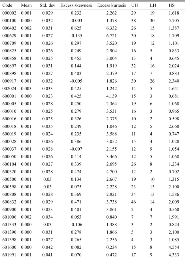
Table1presents the descriptive statistics of stock returns. From table1, we can see that

most series of stock returns have a positive mean and a large standard deviation. Sample means are insigni cantly different from zero, which is a common feature of stock returns across the world. In general, stock returns exhibit skewness to the right and large kurtosis. For all 33 stocks, the number of up price limit hitting is larger than that of down price

limit hit. The percentage of hit days ranges from0.598%to5.705%. Therefore, price limit

hitting is quite frequent for these stocks and is non-trivial. The imposition of price limits is

3_{Poterba and Summers (1988), Conrad et al. (1991) and Lehmann (1990) show signi cant positive}

auto-correlation in daily returns. Campbell et al. (1993) show that trading volume can forcast future returns.

4_{Both Shenzhen Stock Exchange and Shanghai Stock Exchange resumed price limits on December16,}

1996.

5_{ST is a short for "special treatment". It indicats that the company has suffered operating losses for 2}

expected to affect the behavior of stock returns. [ Table1]

3 Model Speci cations

Following Shen and Wang (1998), we employ the following models to investigate the

ef-fects of price limits on the price discovery process:

r_t = ₀+ ₁r_{t 1}+"t; (1)

r_t = ₀+ ( ₂ + ₃T Ot 1)rt 1+"t; (2)

r_t = ₀+ ( ₄ + ₅P LUt 1+ 6P LLt 1)rt 1 +"t; (3)

r_t = ₀+ ( ₇ + ₈T Ot 1+ 9P LUt 1+ 10P LLt 1+)rt 1+"t; (4)

where r_t is the equilibrium stock return that clears the market, T Ot is the turnover at

timet, andP LUt andP LLtare the price limit dummy variables for the upper and lower

price limit hitting, respectively. The dummy variables are equal to 1if the observed price

hits the price limit and0otherwise. Since it is well documented that the stock returns are

characterized by positive autocorrelation over a short interval (Poterba and Summers,1988;

Boudoukh et al.,1994), the autocorrelation coef cients ₁, ₂, ₄, and ₇are expected to be

positive. Previous theoretical studies and empirical evidence suggest that the volume effect is negative (Campbell et al.,1993; Blume et al.,1994; Boudoukh et al.,1994), so we expect

autocorrelation is lower on high-volume days than on low-volume days. Speci cally, we expect ₃ to be negative. If this is true, the daily rst autocorrelation of stock returns decreases when the volume increases, and may even become negative when the trading volume is suf ciently large (see equation2).

Autocorrelation can catch the trend of daily return in the short term. Here we want to investigate whether limit hits intensify the autocorrelation. When the price hits the limit, there are two possibilities. First, if the movement is caused by big news, and the new equilibrium value of the stock is outside the daily price limit range, the stock price will be pushed to the daily price limit. In this case, on the next day, the stock price may continue to move in the same direction, and as a result, the return autocorrelation will be enhanced. On the other hand, the price limit hit may be caused by investors' overreaction. For example, suppose that the fair price of the stock should increase by5%. However, investors overreact

to the news and push the stock price to hit the 10% upper limit. In this case, on the next

day, the stock price may reverse and move in the opposite direction. As a result, the return autocorrelation is weakened. If the delayed price discovery hypothesis holds, ₅, ₆, ₉, and 10are expected to be positive. If the overreaction hypothesis holds, these coef cients are expected to be negative.

In models (1) to (4), the equilibrium returns are required. Note that equilibrium returns

cannot be observed during the price limit hitting days because price limits restrict the range of the price movement. We will rst present the estimation results of OLS and GARCH where the observed prices are treated as if they were the equilibrium prices.6 _{However, as}

pointed out by Chiang and Wei (1995) and Chou (1997), this treatment of data may produce

spurious results because the true relationship among stock returns is distorted. To correct for this problem, we also present estimation results based on the GMM approach proposed by Wei and Chiang (2004) and Shen and Wang (1998). The GMM approach is designed

speci cally to deal with data that are censored by the price limit. It will yield consistent estimates of the true parameters under the assumption that the generating process of stock returns are invariant with price limits. Although the estimations by OLS and GARCH may be biased, they still have some merits and can be complementary to the GMM estimations. OLS can serve as a benchmark, while GARCH considers conditional heteroscedasticity.

4.1 Results of OLS Estimation

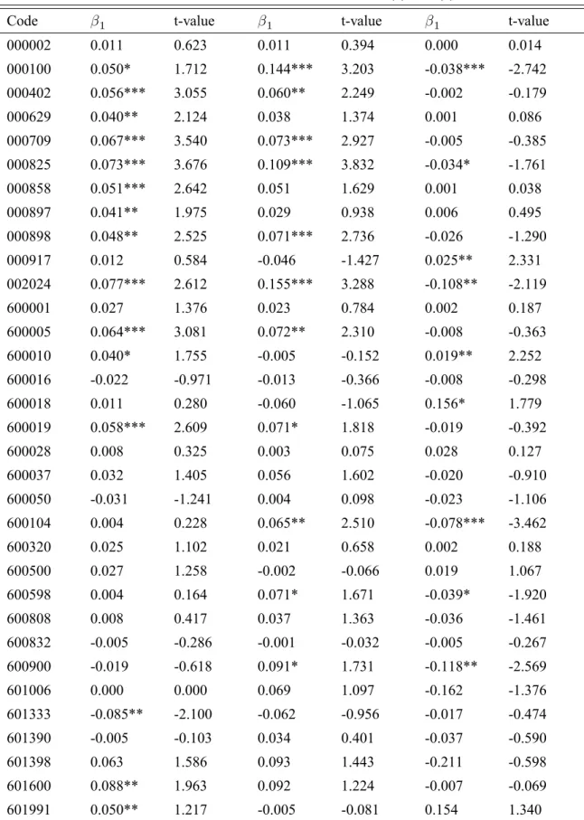
Table 2 reports the OLS estimation results of models (1) and (2). The estimated coef

-cients in model (1) are positive for27out of the33stocks, in which12are signi cant at the 5% level. When the interaction termT Ot 1rt 1 is added, 25 autocorrelation coef cients are positive, in which 8 are signi cant at the 5% level. The autocorrelation coef cients

thus have the expected sign. Furthermore, among the 33 stocks, 21 have negative

coef-cients on the interaction term, T Ot 1rt 1, which suggests that the autocorrelation coef-cient declines when the turnover increases; this is consistent with the negative volume effect reported by previous literature.

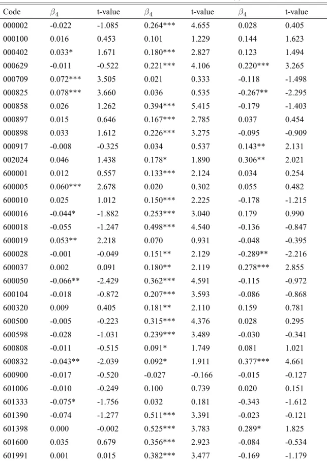
Table3reports the OLS estimation results of model (3), which only considers the price

limits hitting and its effects on the autocorrelation. The coef cients for the autocorrelation,

4, is only positive for 15stocks. However, the upper limit hitting-interaction term, 4; is positive32 out of the33 stocks, and is signi cant for24stocks; this means that when

the price hits the upper limit, the autocorrelation coef cient tends to increase. On the other hand, the coef cient for the lower limit hitting-interacting term is negative for 17

stocks (and signi cantly negative for2stocks), and positive for16stocks (and signi cantly

positive for 6stocks). The OLS estimation results of model (3) suggest that the effect of

the lower limit hitting on the autocorrelation is somewhat inconclusive.

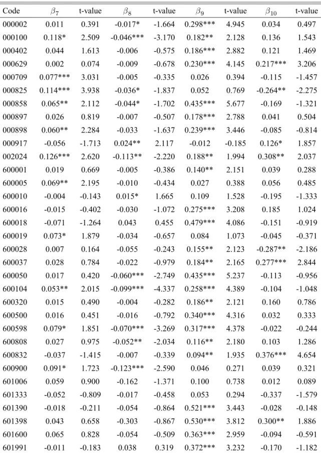
Table4reports the OLS estimation results of model (4). The estimated coef cients, ₇,

is positive for25 out of the33stocks. The turnover reduces the autocorrelation for most

stocks since 8is negative for29stocks, and signi cantly negative for14stocks. Moreover, the coef cient forP LUt 1 is positive except for1 stock, and signi cantly positive for24 stocks. The coef cient of P LLt 1 is positive for20stocks (and signi cantly positive for

6stocks) and negative for13stocks (and signi cantly negative for2stocks). Hence, when

the price hits the upper limit, the autocorrelation tends to increase, while when the price hits the lower limit, the relationship becomes somewhat ambiguous.

Overall, OLS estimation results are consistent with the positive autocorrelation phe-nomenon for short horizons and the common[ly?] testi ed negative volume effect. For the

price limits effect, when price hits the upper limit, the autocorrelation tends to increase; when lower limit hitting happens, the effect is somewhat ambiguous.

[ Table2]

[ Table3]

[ Table4]

4.2 Results of GARCH Estimation

Since asset price typically displays heteroscedasticity, OLS may be inef cient in estimating the autocorrelation coef cient. This section uses the GARCH (1, 1) model to estimate.

Thus the errors are assumed to follow a GARCH (1,1) process as

"tj t 1 N(0; ht);

ht = 0+ 1ht 1+ 2"2t 1:

where t 1 is the information set up to time t 1, ht is the conditional variance, and i

(i= 0;1;2)are unknown positive coef cients.

Since the results of GARCH (1,1) estimation in general agree with the OLS estimation,

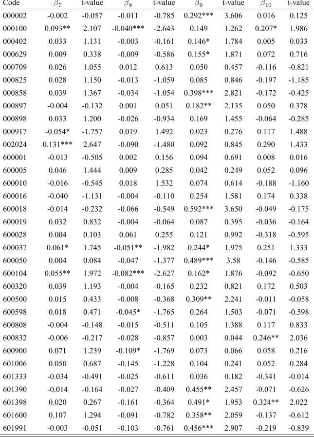
we only report the estimation results of model (4), which are shown in table 5. The 20

out of33estimated coef cients, ₇, are positive. 26out of33coef cients ₈ are negative,

however only 5of them are signi cant. All coef cients onP LUt 1, 9, are positive and

12of them are signi cant. Among33coef cients forP LLt 1,17are positive and16are negative. Among those,3positive ones are signi cant and no negative ones are signi cant.

Therefore, compared to the OLS estimation results, conclusions do not change much except thatGARCH(1;1)estimation results are less signi cant on average.

[table5]

4.3 Results of GMM Estimation

[There should be at least a sentence between a section title and a subsection title]In this section, we present the results from GMM estimation.

4.3.1 Methodology

The OLS and GARCH estimation assumes that the equilibrium returns are equal to the observed returns; this may not be true, especially when the stock price hits the limits. Wei and Chiang (2004) and Shen and Wang (1998) propose the following GMM approach to

deal with this problem..

Assume that the price limits do not affect the true price generating process of the asset. Denote the equilibrium price as P_i;t, and the observed price as Pi;t [what does the

sub-script istand for?, stock i?]. The generating function of the observed return, ri;t, is as

ri;t = 8 > > < > > :

lu if logPi;t=Pi;t >lu,

logP_i;t=Pi;t ifld<logPi;t=Pi;t < lu,

ld if logPi;t=Pi;t ld,

wherelu andld are the upper and lower price limits, respectively. Obviously, whether the

price hits limit depends on whether the equilibrium returnr_i;tlies within the limit range or

not, but not on the magnitude ofr_i;t. Ifr_i;t lies outside the limit range, it is truncated at lu

orld. This truncated data problem can be eliminated by converting the original time series

(sampled daily) into an irregularly observed or unequally spaced time series. Speci cally, for those days when the price limit is hit, we can aggregate returns across consecutive days and treat the multi-day return as a single unit, instead of using the “price-limited” returns on individual days. In the following, we will suppress the subscriptito simplify the notations.

Assuming that the stock price hits the price limit at timet, but it does not for timet 1and

t+ 1, namely,P_{t 6}=Pt,Pt 1 =Pt 1,Pt+1 =Pt+1, thus

rt+1+rt= logPt+1=Pt+ logPt=Pt 1 = logPt+1=Pt 1 =rt+1+rt zt;2:

The two-day true returns,zt;2, can be evaluated even when the daily true returnsrt+1andrt

are not observed. The subscript2inzt;2means thatzt;2is a sum of two terms. The expected value ofzt;2 is2 , which is the mean ofrt. Similarly, for the case where the prices reach

the limits in two consecutive days,tandt+ 1, we have

rt+2+rt+1+rt=rt+2+rt+1+rt zt;3:

The expected value ofzt;3is3 . The analysis is easily extended to thenlimits case. Based on this feature of price limit hitting, Shen and Wang (1998) derived the following four

GMM estimators:

Theory1. Assuming thatr_t is subject to the price limit, andr_t iid N( ; 2), then

the GMM estimators of and 2 _{are given by:}

b =

P

t2S1z

r t;1+

P

t2S2z

r

t;2+ + P

t2Sn+1z

r t;n+1 N1+ 2N2+ + (n+ 1)Nn+1

=

P

t2S1z

r t;1+

P

t2S2z

r

t;2+ + P

t2Sn+1z

r t;n+1

T ;

b2 =

P

t2S1(z

r

t;1 b)2 + P

t2S2(z

r

t;2 2b)2+ + P

t2Sn+1(z

r

t;n+1 (n+ 1)b)2

T ;

wherez_tr_+n =Pn_k=1rt+k 1, Sk+1(k = 1;2; ; n)is the set of rst days ofkconsecutive hitting sequences,n is the maximum number of consecutive price limit hitting in the

sam-ple, Sis the set of all non-limit days,S0 _{is the set of days such that each day of this set is}

is the number of observations in the setSk:

Theory2. Assuming thatr_t is subject to the price limit but xtis not, then the GMM

estimator of covariance ofr_t andxtis

c

cov(r_t; xt) =

1

T X

t2S1

(zr_{t;1 b})(z_t;x_{1 bx})

+1

T X

t2S2

(z_t;r₂ 2_b)(zx_t;2 2_bx)

+

+1

T X

t2Sn+1

(zr_t;n+1 (n+ 1)_b)(z_t;nx ₊₁ (n+ 1)_bx)

wherezx t+n=

Pn

k=1xt+k 1 andbxis the estimated mean ofxt.

Theory3. Assuming that bothr_t andx_t are subject to the price limits, then the

GMM-based estimator of covariance is[I don't quite understand what is going on here).

c

cov(r_t; x_t) = 1

T

X

t2(S1[S1x)

(z_t;r_{1 b})(z_t;x_{1 bx})

+1

T

X

t2(S2[S2x)

(z_t;r₂ 2_b)(z_t;x₂ 2_bx)

+ X

t2S3or t2Sx3; or; t2S2and t+12S2x; or; t+12S2and t2S2x

(z_t;r₃ 3_b)(z_t;x₃ 3_bx) + ]=T

Theory4. Ifr_t is rst-order autocorrelated, then the GMM estimator of variance and

are

b2 =

P

t2S1(z

r

t;1 b)2+ P

t2S2(z

r

t;2 2b)2+ + P

t2Sn+1(z

r

t;n+1 (n+ 1)b)2 N1+ (2 + 2b)N2+ (3 + 4b)N2 + (n+ 1 + 2nb)Nn+1

b = cov_c(r_t; r_t+1)=_b2

Based on these four GMM estimators, we use model (2) to illustrate the GMM

ap-proach. The demeaned equation of model (2) can be written as:

r_t = ₂(r_{t 1} ) + ₃(rto_{t 1 rto}) +"t;

whererto_{t 1} =T Ot 1 rt 1, or in matrix form

e

r_t =x_et0 +"t;

wherere_t =r_t ,x_et = (rt 1 ; rtot 1 rto)0and = ( 2; 3)0. Then

b = (x_etxe0t)

1

(x_etert),

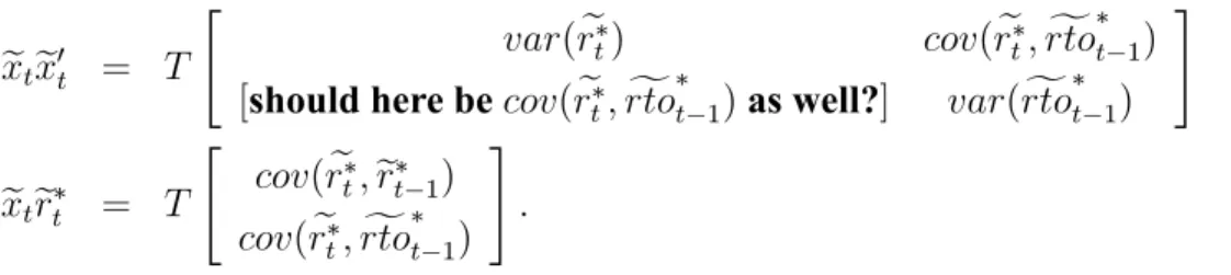
These formulae are the same as the OLS estimators. However, when _ext and ret are

subject to the price limit, the conventional OLS estimators are biased. We can writex_etex0t

andx_etert in the form of variance and covariance:

e

xtex0t = T

"

var(re_t) cov(re_t;rtof_{t 1})

[should here becov(re_t;rtof_{t 1})as well?] var(rtof_{t 1})

#

e

xtret = T

"

cov(re_t;_er_{t 1})

cov(re_t;rtof_{t 1})

# :

These variances and covariances can be calculated based on the previous four theorems. Once the variance and covariance terms are determined, we can obtain consistent estimates bfollowing b= (_extex0t) 1(extert).

4.3.2 GMM estimation results

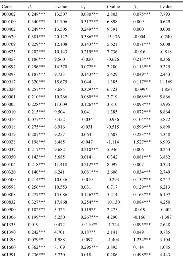
Table 6 reports the GMM estimation results of model (1) and (2). All stocks show

posi-tive autocorrelation (i.e., ₁ > 0), and ₁ is signi cant for all but one stock. For all34

[should be 33?]stocks, ₁is larger than those obtained from OLS or GARCH estimation. Therefore, OLS or GARCH estimation underestimates ₁. When the turnover-interacted variables are considered, the autocorrelation coef cient, ₂;remains positive for25stocks

(and signi cant for 20stocks). Among the 7 cases with a negative ₂, only one is

sig-ni cant. The coef cients of turnover-interacted variables, ₃, are positive for 28 stocks,

and signi cant for22stocks. The coef cient ₃ is negative for5stocks and is signi cant

at the 10% level for one stock. These results are inconsistent with the OLS and GARCH

estimation which suggests negative volume effect. As shown later, this inconsistence is signi cantly weakened if model (4) is used.

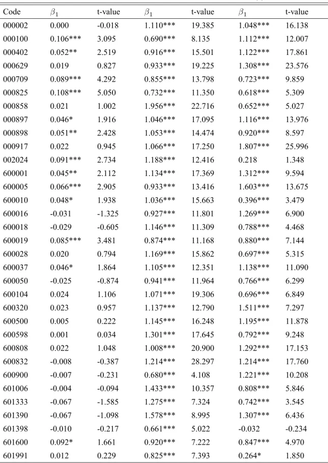
Table7reports the results for model (3) where only the price limit hitting dummies are

considered. The coef cient of the upper price limit hitting, ₅, is positive and signi cant at the1% level for all stocks. The coef cient of the lower price limit hitting, ₆, are positive

and signi cant at the1%level for30stocks (the coef cient is insigni cant for the remaining 3stocks and negative for1stock).

The estimation results for model (4) ares shown in table 8. When we consider both

the turnover-interacted[sometimes I see interacting, sometimes interacted, sometimes interaction; we need to make the term consistent]variable and price limit hitting. The coef cient of the turnover-interacted term, ₆, becomes negative for 17stocks and

signif-icant for4stocks. For16stocks, ₆ remains positive, but is only signi cant for 2stocks.

Therefore, the volume effect is not very strong in China's stock markets. Similar to the ndings for model (3), the coef cient of the upper price limit hitting, ₉, is positive and

signi cant at 1% level for all stocks. The coef cient for lower price limit hitting, ₁₀, is

positive and signi cant at the1%level for30stocks. For3stocks, ₁₀is insigni cant and

negative for one stock. [table6]

[table7]

5 Conclusion

This paper studies the effect of price limits on price discovery process in China's stock market by examining whether the price limit strengthens the daily return autocorrelation or not. Using two conventional methods, OLS and GARCH, we nd the positive autocorre-lation in the short horizon and the negative volume effect as in previous literature. When the price hits the upper limit, the autocorrelation is strengthened. When the price hits the lower limit, the effect on autocorrelation is inconclusive. The result seems to suggest that the delayed price discovery hypothesis holds for the upper price limit, however, both the overreaction hypothesis and the delayed price discovery hypothesis are reasonable for the lower price limit.

References

Al-Khouri, R., S., M., M., Ajlouni, “Narrow Price Limit and Stock Price Volatil-ity: Empirical Evidence from Amman Stock Exchange”, International Research Journal of Finance and Economics8,2007, p.163-180.

Blume, L., D., Easley, M., O'Hara, “Market Statistics and Technical Analysis: The Role of Volume”, The Journal of Finance, March,1994, p.153-181.

Boudoukh, J., M., P., Richardson, R., F., Whitelaw, “A Tale of Three Schools: Insights on Autocorrelations of Short-horizon Stock Returns”, The Review of Financial Studies7, 1994, p. 539-573.

Campbell, J., Y., S., J., Grossman, J., Wang, “Trading Volume and Serial Correlation in Stock Returns”, The Quarterly Journal of Economics, November,1993, p.905-940.

Chen, G., O., M., Rui, S., S., Wang, “The Effectiveness of Price Limits and Stock Char-acteristics: Evidence from Shanghai and Shenzhen Stock Exchange”, Review of Quantita-tive Finance and Accounting25,2005, p.159-182.

Chou, P., H., A Gibbs Sampling Approach to The Estimation of Linear Regression Models Under Price Limits”, Paci c-Basin Finance Journal5,1997, p.39-62.

Chou, P., H., “Modeling Daily Price Limits”, International Review of Financial Analy-sis8:3,1999, p.283-301.

Conrad, J., S., G., Kaul, M., Numalendran, “Components of Short-horizon Individual Security Returns”, Journal of Financial Economics29,1991, p.365-384.

George P.D, N., Patsalis, N., V., Tsangarakis, E., D., Tsiritakis, “Price Limits and Over-reaction in Athens Stock Exchange”, Applied Financial Economics15,2005, p.53-61.

Fama, E., “Perspectives on October 1987, or, What Did We Learn from The Crash?”

Black Monday and the Future of Financial Markets,1989, p.71-82.

Feng, L., “The Effect of10% Price Limits on the Chinese Stock Market”, Asian-Paci c

Journal of Economics and Business6, June,2002, p.26-41.

George P.D, N., Patsalis, N., V., Tsangarakis, E., D., Tsiritakis, “Price Limits and Over-reaction in Athens Stock Exchange”, Applied Financial Economics15,2005, p.53-61.

Hsieh, P., H., J., J., Yang, “A Censored Stochastic Volatility Approach to The Estima-tion of Price Limit Moves”, Journal of Empirical Finance16,2009, p.337-351.

Huang, Y., T., Fu, M., Ke, “Daily Price Limits and Stock Price Behavior: Evidence from The Taiwan Stock Exchange”, International Review of Economics and Finance 10, 2001, p.263-288.

Kim, K., A. and S., G., Rhee, “Price Limit Performance: Evidence from The Tokyo Stock Exchange”, The Journal of Finance52, No.2,1997, p.885-901.

Lauterbach,B. and U.Ben-Zion, “Stock Market Crashes and the performance of Circuit Breakers: Empirical Evidence.”, Journal of Finance48,1993,1909-1925.

Lehmann, B., N., “Fads, Martingales, and Market Ef ciency”, The Quarterly Journal of Economics, February,1990, p.1-28.

Ma, C., R.Rao and R.Sears “Commentary: Volatility, Price Resolution, and The Effec-tiveness of Price Limits”, Journal of Financial Services Research3,1989, p. 205-209.

Phylaktis, K.M Kavusannos and G Manalis, “Price Limit and Stock Market Volatility in the Athens Stock Exchange”, European Financial Management5,1999, p. 33-59.

Qu W.2007, "Effect of Market Institution on the Ef ciency of China's Stock Markets",

Journal of Xianmen University (in Chinese), issue3, p40-47.

Shen, C. and L., Wang, “Daily Serial Correlation, Trading Volume and Price Limits: Evidence from Taiwan Stock Market”, Paci c-Basin Finance Journal6,1998, p.251-273.

Wei, K., C., J., R., Chiang, “A GMM Approach for Estimation of Volatility and Re-gression Models When Daily Prices Are Subject to Price Limits”, Paci c-Basin Finance Journal12,2004, p.445-461.

Wei, S., X., “A Censored-GARCH Model of Asset Returns With Price Limits”, Journal of Empirical Finance9,2002, p.197-223.

Wu L. and L.Xu, 2002, “Doe Price limit Distort the Behavior of Stcok Price”, China

Accounting and Finance Review (in Chinese), issue2, p.1-42.

Table 1: Descriptive statistics of stocks returns

Code Mean Std. dev Excess skewness Excess kurtosis UH LH HS

000002 0.001 0.029 0.232 2.262 29 19 1.618

000100 0.000 0.032 -0.003 1.378 38 30 5.705

000402 0.002 0.031 0.625 6.332 26 15 1.387

000629 0.001 0.027 -0.135 6.721 30 18 1.709

000709 0.001 0.026 0.297 3.520 19 12 1.101

000825 0.001 0.026 0.249 2.904 16 5 0.833

000858 0.001 0.025 0.455 3.004 13 4 0.645

000897 0.001 0.031 0.144 1.919 32 16 2.024

000898 0.001 0.027 0.403 2.379 17 7 0.883

000917 0.001 0.032 -0.005 1.826 30 26 2.340

002024 0.003 0.033 0.425 1.242 14 5 1.641

600001 0.000 0.023 0.425 4.139 15 3 0.681

600005 0.001 0.028 0.250 2.364 19 6 1.068

600010 0.001 0.025 0.279 3.531 16 3 0.965

600016 0.001 0.025 0.326 2.375 10 2 0.598

600018 0.001 0.035 0.249 1.046 12 5 2.660

600019 0.001 0.024 0.235 3.588 11 4 0.747

600028 0.001 0.026 0.386 3.052 15 4 1.028

600037 0.001 0.028 -0.007 2.155 12 9 1.054

600050 0.001 0.026 0.414 3.466 12 5 1.068

600104 0.001 0.027 0.339 2.695 26 8 1.234

600320 0.001 0.028 0.474 4.700 12 2 0.702

600500 0.001 0.03 0.134 2.667 19 10 1.315

600598 0.001 0.03 0.075 2.228 23 13 2.100

600808 0.001 0.028 0.369 2.821 34 13 1.586

600832 0.001 0.029 0.471 3.738 46 14 2.009

600900 0.001 0.023 0.401 3.861 2 4 0.560

601006 0.002 0.034 0.053 0.840 7 7 1.991

601333 0.000 0.03 -0.106 1.388 3 2 0.824

601390 0.000 0.031 0.278 1.866 5 3 2.100

601398 0.001 0.027 0.265 2.256 4 3 1.085

601600 0.000 0.042 0.082 0.234 15 8 4.554

601991 0.001 0.041 0.070 0.472 17 9 4.333

Notes:

Table 2: OLS estimation results of model (1) and (2)

Code ₁ t-value ₁ t-value ₁ t-value

000002 0.011 0.623 0.011 0.394 0.000 0.014

000100 0.050* 1.712 0.144*** 3.203 -0.038*** -2.742

000402 0.056*** 3.055 0.060** 2.249 -0.002 -0.179

000629 0.040** 2.124 0.038 1.374 0.001 0.086

000709 0.067*** 3.540 0.073*** 2.927 -0.005 -0.385

000825 0.073*** 3.676 0.109*** 3.832 -0.034* -1.761

000858 0.051*** 2.642 0.051 1.629 0.001 0.038

000897 0.041** 1.975 0.029 0.938 0.006 0.495

000898 0.048** 2.525 0.071*** 2.736 -0.026 -1.290

000917 0.012 0.584 -0.046 -1.427 0.025** 2.331

002024 0.077*** 2.612 0.155*** 3.288 -0.108** -2.119

600001 0.027 1.376 0.023 0.784 0.002 0.187

600005 0.064*** 3.081 0.072** 2.310 -0.008 -0.363

600010 0.040* 1.755 -0.005 -0.152 0.019** 2.252

600016 -0.022 -0.971 -0.013 -0.366 -0.008 -0.298

600018 0.011 0.280 -0.060 -1.065 0.156* 1.779

600019 0.058*** 2.609 0.071* 1.818 -0.019 -0.392

600028 0.008 0.325 0.003 0.075 0.028 0.127

600037 0.032 1.405 0.056 1.602 -0.020 -0.910

600050 -0.031 -1.241 0.004 0.098 -0.023 -1.106

600104 0.004 0.228 0.065** 2.510 -0.078*** -3.462

600320 0.025 1.102 0.021 0.658 0.002 0.188

600500 0.027 1.258 -0.002 -0.066 0.019 1.067

600598 0.004 0.164 0.071* 1.671 -0.039* -1.920

600808 0.008 0.417 0.037 1.363 -0.036 -1.461

600832 -0.005 -0.286 -0.001 -0.032 -0.005 -0.267

600900 -0.019 -0.618 0.091* 1.731 -0.118** -2.569

601006 0.000 0.000 0.069 1.097 -0.162 -1.376

601333 -0.085** -2.100 -0.062 -0.956 -0.017 -0.474

601390 -0.005 -0.103 0.034 0.401 -0.037 -0.590

601398 0.063 1.586 0.093 1.443 -0.211 -0.598

601600 0.088** 1.963 0.092 1.224 -0.007 -0.069

601991 0.050** 1.217 -0.005 -0.081 0.154 1.340

Notes:

Table 3: OLS estimation results of model (3)

Code ₄ t-value ₄ t-value ₄ t-value

000002 -0.022 -1.085 0.264*** 4.655 0.028 0.405

000100 0.016 0.453 0.101 1.229 0.144 1.623

000402 0.033* 1.671 0.180*** 2.827 0.123 1.494

000629 -0.011 -0.522 0.221*** 4.106 0.220*** 3.265

000709 0.072*** 3.505 0.021 0.333 -0.118 -1.498

000825 0.078*** 3.660 0.036 0.535 -0.267** -2.295

000858 0.026 1.262 0.394*** 5.415 -0.179 -1.403

000897 0.015 0.646 0.167*** 2.785 0.037 0.454

000898 0.033 1.612 0.226*** 3.275 -0.095 -0.909

000917 -0.008 -0.325 0.034 0.537 0.143** 2.131

002024 0.046 1.438 0.178* 1.890 0.306** 2.021

600001 0.012 0.557 0.133*** 2.124 0.034 0.254

600005 0.060*** 2.678 0.020 0.302 0.055 0.482

600010 0.025 1.012 0.150*** 2.225 -0.178 -1.215

600016 -0.044* -1.882 0.253*** 3.040 0.179 0.990

600018 -0.055 -1.247 0.498*** 4.540 -0.136 -0.847

600019 0.053** 2.218 0.070 0.931 -0.048 -0.395

600028 -0.001 -0.049 0.151** 2.129 -0.289** -2.216

600037 0.002 0.091 0.180** 2.119 0.278*** 2.855

600050 -0.066** -2.429 0.362*** 4.591 -0.115 -0.972

600104 -0.018 -0.872 0.207*** 3.593 -0.086 -0.868

600320 0.009 0.405 0.181** 2.110 0.159 0.781

600500 -0.005 -0.223 0.315*** 4.376 0.028 0.295

600598 -0.028 -1.031 0.239*** 3.489 -0.030 -0.341

600808 -0.011 -0.515 0.091* 1.749 0.081 1.021

600832 -0.043** -2.039 0.092* 1.911 0.377*** 4.661

600900 -0.017 -0.520 -0.027 -0.166 -0.015 -0.127

601006 -0.010 -0.249 0.100 0.739 0.020 0.151

601333 -0.075* -1.756 0.032 0.181 -0.343 -1.612

601390 -0.074 -1.277 0.511*** 3.391 -0.023 -0.121

601398 0.000 -0.002 0.525*** 3.783 0.289* 1.825

601600 0.035 0.679 0.356*** 2.923 -0.084 -0.534

601991 0.001 0.015 0.382*** 3.477 -0.169 -1.179

Notes:

Table 4: OLS estimation results of model (4)

Code ₇ t-value ₈ t-value ₉ t-value ₁₀ t-value

000002 0.011 0.391 -0.017* -1.664 0.298*** 4.945 0.034 0.497 000100 0.118* 2.509 -0.046*** -3.170 0.182** 2.128 0.136 1.543 000402 0.044 1.613 -0.006 -0.575 0.186*** 2.882 0.121 1.469 000629 0.002 0.074 -0.009 -0.678 0.230*** 4.145 0.217*** 3.206 000709 0.077*** 3.031 -0.005 -0.335 0.026 0.394 -0.115 -1.457 000825 0.114*** 3.938 -0.036* -1.837 0.052 0.769 -0.264** -2.275 000858 0.065** 2.112 -0.044* -1.702 0.435*** 5.677 -0.169 -1.321 000897 0.026 0.819 -0.007 -0.507 0.178*** 2.788 0.041 0.504 000898 0.060** 2.284 -0.033 -1.637 0.239*** 3.446 -0.085 -0.814 000917 -0.056 -1.713 0.024** 2.117 -0.012 -0.185 0.126* 1.857 002024 0.126*** 2.620 -0.113** -2.220 0.188** 1.994 0.308** 2.037 600001 0.019 0.669 -0.005 -0.386 0.140** 2.151 0.039 0.288 600005 0.069** 2.195 -0.010 -0.434 0.027 0.388 0.056 0.485 600010 -0.004 -0.143 0.015* 1.665 0.109 1.528 -0.195 -1.333 600016 -0.015 -0.402 -0.030 -1.072 0.275*** 3.208 0.185 1.024 600018 -0.071 -1.264 0.043 0.455 0.479*** 4.086 -0.151 -0.919 600019 0.073* 1.879 -0.034 -0.657 0.084 1.073 -0.045 -0.371 600028 0.007 0.164 -0.055 -0.243 0.155** 2.123 -0.287** -2.186 600037 0.028 0.784 -0.022 -0.979 0.184** 2.165 0.277*** 2.844 600050 0.017 0.420 -0.060*** -2.749 0.435*** 5.237 -0.113 -0.956 600104 0.053** 2.015 -0.099*** -4.337 0.258*** 4.389 -0.104 -1.048 600320 0.015 0.490 -0.004 -0.282 0.186** 2.121 0.160 0.786 600500 0.016 0.451 -0.016 -0.792 0.340*** 4.316 0.032 0.333 600598 0.079* 1.851 -0.070*** -3.269 0.317*** 4.378 -0.022 -0.244 600808 0.027 0.975 -0.052** -2.034 0.116** 2.180 0.103 1.286 600832 -0.037 -1.415 -0.007 -0.339 0.094** 1.935 0.376*** 4.654 600900 0.091* 1.723 -0.123*** -2.590 0.046 0.271 0.039 0.321 601006 0.059 0.900 -0.162 -1.371 0.100 0.738 0.012 0.089 601333 -0.052 -0.809 -0.017 -0.458 0.053 0.294 -0.337 -1.579 601390 -0.018 -0.211 -0.054 -0.864 0.521*** 3.443 -0.028 -0.148 601398 0.043 0.658 -0.303 -0.867 0.530*** 3.812 0.300** 1.886 601600 0.065 0.828 -0.054 -0.509 0.363*** 2.959 -0.094 -0.591 601991 -0.011 -0.183 0.038 0.319 0.372*** 3.232 -0.170 -1.182

Notes:

Table 5: GARCH (1,1) estimation results of model (4)

Code ₇ t-value ₈ t-value ₉ t-value ₁₀ t-value

000002 -0.002 -0.057 -0.011 -0.785 0.292*** 3.606 0.016 0.125 000100 0.093** 2.107 -0.040*** -2.643 0.149 1.262 0.207* 1.986 000402 0.033 1.131 -0.003 -0.161 0.146* 1.784 0.005 0.033 000629 0.009 0.338 -0.009 -0.586 0.155* 1.871 0.072 0.716 000709 0.026 1.055 0.012 0.613 0.050 0.457 -0.116 -0.821 000825 0.028 1.150 -0.013 -1.059 0.085 0.846 -0.197 -1.185 000858 0.039 1.367 -0.034 -1.054 0.398*** 2.821 -0.172 -0.425 000897 -0.004 -0.132 0.001 0.051 0.182** 2.135 0.050 0.378 000898 0.033 1.200 -0.026 -0.934 0.169 1.455 -0.064 -0.285 000917 -0.054* -1.757 0.019 1.492 0.023 0.276 0.117 1.488 002024 0.131*** 2.647 -0.090 -1.480 0.092 0.845 0.290 1.433 600001 -0.013 -0.505 0.002 0.156 0.094 0.691 0.008 0.016 600005 0.046 1.444 0.009 0.285 0.042 0.249 0.052 0.096 600010 -0.016 -0.545 0.018 1.532 0.074 0.614 -0.188 -1.160 600016 -0.040 -1.131 -0.004 -0.110 0.254 1.581 0.174 0.338 600018 -0.014 -0.232 -0.066 -0.549 0.592*** 3.650 -0.049 -0.175 600019 0.032 0.832 -0.004 -0.064 0.087 0.395 -0.036 -0.164 600028 0.004 0.103 0.061 0.255 0.121 0.992 -0.318 -0.595 600037 0.061* 1.745 -0.051** -1.982 0.244* 1.975 0.251 1.333 600050 0.004 0.084 -0.047 -1.377 0.489*** 3.58 -0.146 -0.585 600104 0.055** 1.972 -0.082*** -2.627 0.162* 1.876 -0.092 -0.650 600320 0.039 1.193 -0.004 -0.165 0.232 0.821 0.172 0.503 600500 0.015 0.433 -0.008 -0.368 0.309** 2.241 -0.011 -0.058 600598 0.018 0.471 -0.045* -1.765 0.264 1.503 -0.071 -0.598 600808 -0.004 -0.148 -0.015 -0.511 0.105 1.388 0.117 0.833 600832 -0.006 -0.217 -0.028 -0.857 0.003 0.044 0.246** 2.036 600900 0.071 1.239 -0.109* -1.769 0.073 0.066 0.058 0.216 601006 0.050 0.687 -0.145 -1.228 0.104 0.241 0.052 0.284 601333 -0.034 -0.491 -0.025 -0.611 0.036 0.182 -0.341 -0.014 601390 -0.014 -0.164 -0.027 -0.409 0.455** 2.457 -0.071 -0.626 601398 0.020 0.267 -0.161 -0.364 0.491* 1.953 0.324** 2.022 601600 0.107 1.294 -0.091 -0.782 0.358** 2.059 -0.137 -0.612 601991 -0.003 -0.051 -0.103 -0.761 0.456*** 2.907 -0.219 -0.839

Notes:

Table 6: GMM-Price limit estimation results of model (1) and (2)

Code ₁ t-value ₁ t-value ₁ t-value

000002 0.248*** 13.507 0.080*** 2.803 0.075*** 7.793

000100 0.340*** 11.706 0.317*** 6.898 0.009 0.629

000402 0.249*** 13.505 0.249*** 9.391 0.000 0.000

000629 0.381*** 20.127 0.386*** 13.176 -0.004 -0.240 000709 0.229*** 12.108 0.143*** 5.621 0.071*** 5.008 000825 0.202*** 10.143 0.219*** 7.736 -0.016 -0.818 000858 0.186*** 9.560 -0.020 -0.626 0.213*** 8.366 000897 0.296*** 14.370 0.072** 2.280 0.113*** 9.325 000898 0.187*** 9.733 0.143*** 5.429 0.049** 2.443

000917 0.320*** 15.675 0.044 1.385 0.117*** 11.169

002024 0.257*** 8.685 0.329*** 6.723 -0.099* -1.850 600001 0.210*** 10.766 0.080*** 2.719 0.068*** 5.866 600005 0.228*** 11.009 0.126*** 3.810 0.098*** 3.995

600010 0.215*** 9.504 0.041 1.385 0.072*** 8.864

600016 0.077*** 3.452 -0.034 -0.936 0.104*** 3.872 600018 0.275*** 6.916 -0.031 -0.515 0.596*** 6.890

600019 0.207*** 9.257 0.064 1.607 0.223*** 4.348

600028 0.198*** 8.485 -0.047 -1.114 1.527*** 6.993

600037 0.217*** 9.682 0.210*** 5.946 0.006 0.254

600050 0.143*** 5.685 0.014 0.342 0.081*** 3.882

600104 0.218*** 11.418 0.212*** 8.097 0.007 0.323

600320 0.140*** 6.241 0.081*** 2.606 0.034*** 2.749 600500 0.214*** 10.036 -0.010 -0.293 0.137*** 8.247

600598 0.256*** 10.553 0.031 0.717 0.129*** 6.213

600808 0.277*** 15.086 0.146*** 5.214 0.163*** 6.197 600832 0.327*** 17.868 0.254*** 10.130 0.084*** 4.250

600900 0.102*** 3.325 0.119** 2.275 -0.019 -0.402

601006 0.199*** 5.250 0.267*** 4.290 -0.166 -1.387

601333 0.019 0.472 -0.110** -1.724 0.095*** 2.648

601390 0.242*** 4.701 0.187** 2.141 0.049 0.785

601398 0.079** 1.988 -0.097 -1.404 1.234*** 3.104

601600 0.362*** 8.109 0.295*** 3.895 0.114 1.085

601991 0.236*** 5.730 0.018 0.286 0.498*** 4.443

Notes:

Table 7: GMM-Price limit estimation results of model (3)

Code ₁ t-value ₁ t-value ₁ t-value

000002 0.000 -0.018 1.110*** 19.385 1.048*** 16.138 000100 0.106*** 3.095 0.690*** 8.135 1.112*** 12.007 000402 0.052** 2.519 0.916*** 15.501 1.122*** 17.861

000629 0.019 0.827 0.933*** 19.225 1.308*** 23.576

000709 0.089*** 4.292 0.855*** 13.798 0.723*** 9.859 000825 0.108*** 5.050 0.732*** 11.350 0.618*** 5.309

000858 0.021 1.002 1.956*** 22.716 0.652*** 5.027

000897 0.046* 1.916 1.046*** 17.095 1.116*** 13.976 000898 0.051** 2.428 1.053*** 14.474 0.920*** 8.597

000917 0.022 0.945 1.066*** 17.250 1.807*** 25.996

002024 0.091*** 2.734 1.188*** 12.416 0.218 1.348

600001 0.045** 2.112 1.134*** 17.369 1.312*** 9.594 600005 0.066*** 2.905 0.933*** 13.416 1.603*** 13.675 600010 0.048* 1.938 1.036*** 15.663 0.396*** 3.479 600016 -0.031 -1.325 0.927*** 11.801 1.269*** 6.900 600018 -0.029 -0.605 1.146*** 11.309 0.788*** 4.468 600019 0.085*** 3.481 0.874*** 11.168 0.880*** 7.144

600028 0.020 0.794 1.169*** 15.862 0.697*** 5.315

600037 0.046* 1.864 1.105*** 12.351 1.138*** 11.090 600050 -0.025 -0.874 0.941*** 11.964 0.766*** 6.299

600104 0.024 1.106 1.071*** 19.306 0.696*** 6.849

600320 0.023 0.957 1.137*** 12.790 1.511*** 7.297

600500 0.005 0.222 1.145*** 16.248 1.195*** 11.878

600598 0.001 0.034 1.301*** 17.645 0.792*** 9.248

600808 0.022 1.048 1.008*** 20.900 1.292*** 17.153

600832 -0.008 -0.387 1.214*** 28.297 1.214*** 17.760 600900 -0.007 -0.231 0.680*** 4.108 1.221*** 10.208 601006 -0.004 -0.094 1.433*** 10.357 0.808*** 5.846 601333 -0.067 -1.585 1.275*** 7.324 0.742*** 3.545 601390 -0.067 -1.098 1.578*** 8.995 1.307*** 6.436

601398 -0.010 -0.217 0.661*** 5.022 -0.032 -0.234

601600 0.092* 1.661 0.920*** 7.222 0.847*** 4.970

601991 0.012 0.229 0.825*** 7.393 0.264* 1.850

Notes:

Table 8: GMM-Price limit estimation results of model (4)

Code ₇ t-value ₈ t-value ₉ t-value ₁₀ t-value

000002 -0.002 -0.052 0.001 0.057 1.109*** 17.514 1.048*** 16.136 000100 0.142*** 2.952 -0.017 -1.067 0.719*** 8.077 1.109*** 11.973 000402 0.056** 2.007 -0.003 -0.240 0.919*** 15.342 1.120*** 17.711 000629 0.037 1.159 -0.013 -0.813 0.941*** 18.990 1.302*** 23.293 000709 0.084*** 3.260 0.005 0.325 0.850*** 13.260 0.719*** 9.684 000825 0.166*** 5.814 -0.060*** -3.073 0.772*** 11.733 0.617*** 5.300 000858 0.016 0.510 0.005 0.199 1.949*** 21.136 0.651*** 5.021 000897 0.006 0.179 0.025* 1.894 0.993*** 14.756 1.099*** 13.681 000898 0.069** 2.569 -0.022 -1.075 1.070*** 14.367 0.928*** 8.646 000917 -0.070** -2.165 0.046*** 4.042 0.967*** 14.555 1.776*** 25.384 002024 0.195*** 3.865 -0.147*** -2.743 1.207*** 12.579 0.231 1.427 600001 0.046 1.540 0.000 -0.027 1.134*** 16.613 1.312*** 9.534 600005 0.048 1.451 0.018 0.709 0.921*** 12.853 1.601*** 13.657 600010 0.004 0.140 0.023*** 2.617 0.958*** 13.201 0.387*** 3.399 600016 -0.044 -1.209 0.013 0.457 0.916*** 11.166 1.267*** 6.893 600018 -0.064 -1.064 0.098 0.965 1.085*** 9.111 0.755*** 4.206 600019 0.063 1.571 0.037 0.680 0.856*** 10.360 0.877*** 7.113 600028 -0.035 -0.837 0.387* 1.665 1.124*** 14.357 0.691*** 5.269 600037 0.068* 1.856 -0.018 -0.801 1.112*** 12.370 1.137*** 11.083 600050 0.010 0.246 -0.026 -1.121 0.983*** 11.311 0.765*** 6.295 600104 0.087*** 3.216 -0.089*** -3.829 1.120*** 19.672 0.681*** 6.697 600320 0.028 0.889 -0.003 -0.247 1.142*** 12.467 1.511*** 7.295 600500 0.033 0.919 -0.021 -1.042 1.194*** 14.141 1.203*** 11.923 600598 0.034 0.762 -0.022 -0.955 1.333*** 16.401 0.795*** 9.281 600808 0.024 0.853 -0.003 -0.123 1.010*** 20.413 1.293*** 17.010 600832 -0.026 -0.959 0.021 1.072 1.207*** 27.885 1.216*** 17.783 600900 0.101* 1.931 -0.125*** -2.638 0.755*** 4.494 1.271*** 10.494 601006 0.051 0.777 -0.131 -1.091 1.433*** 10.358 0.799*** 5.768 601333 -0.096 -1.508 0.023 0.610 1.248*** 6.948 0.731*** 3.479 601390 -0.005 -0.051 -0.060 -0.945 1.609*** 9.018 1.325*** 6.496 601398 -0.155*** -2.162 1.056*** 2.643 0.627*** 4.741 -0.043 -0.314 601600 0.066 0.811 0.047 0.437 0.911*** 7.049 0.855*** 4.988 601991 -0.020 -0.305 0.105 0.810 0.773*** 5.971 0.248 1.724

Notes: