The Effect of Superstar Firms on
College Major Choice
*Darwin Choi
Chinese University of Hong Kong [email protected]
Dong Lou
London School of Economics and CEPR [email protected]
Abhiroop Mukherjee
Hong Kong University of Science and Technology [email protected]
This Draft: October 2017
* We thank Ashwini Agrawal, Nick Barberis, James Choi, Xavier Gabaix, Robin Greenwood, David
The Effect of Superstar Firms on
College Major Choice
Abstract
We study the effect of superstar firms on an important human capital decision – college students’ choice of major. Past salient, extreme events in an industry, as proxied by cross-sectional skewness in stock returns (or in favorable news coverage), are associated with a disproportionately larger number of college students choosing to major in related fields, even after controlling for the average industry return. This tendency to follow the superstars, however, results in a temporary over-supply of human capital. Specifically, we provide evidence that the additional labor supply due to salient, extreme events lowers the average wage earned by entry-level employees when students enter the job market. At the same time, employment size and employee turnover stay roughly constant in related industries, consistent with the view that labor demand is relatively inelastic in the short run. In the longer term, firms cope with the supply increase by gradually expanding the number of positions that require prior experience.
JEL Classification: G11, G12, G14, G20
1. Introduction
It has long been of interest to economists the effect of salient, extreme events on human
decision making. For example, there is a recent, fast-growing literature that examines
the role of salient, extreme events in driving agents’ financial decisions (e.g., Barberis
and Huang, 2008; Bordalo, Gennaioli, and Shleifer, 2012). There is, however, much less
work on the impact of such events on other, potentially more important, aspects of
human decision making. In this paper, we shed new light on this issue by focusing on
one of the most irreversible investment decisions an individual ever has to make – her
education and human capital investment.
Our paper studies the effect of superstar firms on college students’ major choice.
There is plenty of anecdotal evidence that links extreme success (or failure) episodes in
an industry to variations in the number of graduates in related fields. For example, as
reported by Stanford Daily, the number of graduates with a Computer Science major in
2013 was nearly four times that in 2006, potentially attributable to the extreme
successes of a handful of mobile app and social media companies (a prominent example
of which is Facebook). A New York Times article on June 15, 2011 indeed argues that
“students are flocking to computer science because they dream of being the next Mark
Zuckerberg.”
The objective of our paper is to bring to the data the casual claim that college
students’ attention is drawn to – and their expectations and decisions shaped by – the
occurrences of superstar (and similarly super-loser) firms in related industries.
Intuitively, superstar firms can affect college students’ major choice through two related
channels. First, the occurrences of superstar firms often involve extreme payoffs – Mark
Facebook went public. A long-standing literature in labor economics, dating back to at
least Rosen (1997), argues that individuals have a preference for skewed payoffs,
possibly due to the complementarity between taste and income (i.e., state-dependent
utility). Second, extreme success stories garner disproportionate media coverage and
social attention: the story of Mark Zuckerberg, who dropped out of college to work
full-time on his Facebook project, has been a constant talking point on college campus.
Consequently, salient extreme events play a disproportionate large role in shaping
student’s expectations and decisions, especially in the presence of substantial search
costs faced by college students.
To operationalize our empirical analyses, we take the following steps. First, we
focus solely on the set of science and engineering majors (e.g., computer science vs.
chemical engineering) that can be mapped relatively cleanly to one or more industry
sectors (e.g., information technology vs. pharmaceutical). Second, to quantify salient,
extreme events in every industry in each period, we resort to stock returns as a
capture-it-all measure of value-relevant events. Specifically, we measure the occurrence of
superstars (or super-losers) in each industry by the cross-sectional return skewness in
that industry (a similar measure is also employed by Zhang, 2006 and Green and
Hwang, 2012). Positive cross-sectional skewness indicates that, holding the industry’s
average return and return volatility constant, a small number of firms in the industry
perform exceptionally well; these salient, extreme examples then draw college students
to the related majors. Negative cross-sectional skewness, on the other hand, indicates
that a small number of firms in the industry have done exceptionally poorly, which is
likely to drive students away from the related majors. Third, since college students
to graduation), we focus on industry return skewness measured in years t-7 to t-3 prior
to the graduation year (i.e., from their junior year in high school to the end of
sophomore year in college) to explain major enrollment in year t.1
Our empirical results strongly support the view that salient, extreme events
affect college major choice and, in turn, labor supply in related industries. Using college
enrollment data compiled by the National Science Foundation (NSF), we show that a
one-standard-deviation increase in within-industry (cross-sectional) return skewness in
years t-7 to t-3 is associated with a statistically significant 10.6% increase in the number
of students graduating in related majors in year t. This result is robust to controlling for
the average industry return and return volatility measured over the same period, as well
as time and major fixed effects.
A potential concern with our supply-side interpretation is that the increase in
major enrollment associated with industry skewness may also be consistent with a
demand-side explanation. That is, college students rationally anticipate that some
industries will prosper in the near future and choose to invest their human capital in
these industries by studying related subjects. First, it is unclear why cross-sectional
return skewness should forecast future industry prospects after controlling for the
average industry return and return volatility. Indeed, in simple linear regressions, we
show that industry return skewness is uncorrelated with future industry operating
performance, as measured by the return on equity (ROE), profit margin, and
earnings/sales growth.
Nonetheless, to tease out the labor-demand channel from our supply-side
explanation (i.e., labor supply being driven by salient, extreme events in the industry),
we examine the wage and number of employees in these related industries in subsequent
years. By examining both the price and quantity in the labor market, we can then
distinguish relative shifts in the supply curve vs. demand curve.2
Moreover, the
granularity of the industry employment data from Bureau of Labor Statistics (BLS)
allows us to separately examine the wage and number of employees with college degrees
for entry-level positions vs. advanced positions that require prior experience.
Our results are most consistent with a relatively larger shift in labor supply that
is induced by extreme, salient industry events. A one-standard-deviation increase in
industry return skewness in years t7 to t3 is associated with a 1.9% (tstatistic =
-3.39) drop in the average wage earned by entry-level employees in related industries in
year t. To put this number in perspective, a one-standard-deviation increase in the
industry average return is associated with a much lower 0.47% increase in wages.
Moreover, the effect of industry return skewness on the average entry-level wage
decreases with the extent to which an industry overlaps with other industries in terms
of absorbing students from a particular major. This is because for industries with close
substitutes, an increase in student supply is shared among all similar industries and thus
leads to a smaller wage decline.
Meanwhile, the effect of industry return skewness in years t-7 to t-3 on the
number of entry-level employees (as well as employee turnover) in year t is
indistinguishable from zero. This is consistent with the view that labor demand is
2 While both the demand and supply curves may shift, the price-quantity pair can inform us which curve
relatively inelastic in the short run; a sudden increase in labor supply thus lowers the
average wage earned by entry-level employees without changing the size of employment.
(This is not to say that the additional student supply is not absorbed by the labor
market; e.g., the additional graduates may compete with job-seekers without a college
degree, whom we do not have data on.)
To understand the long-term impact of labor supply shocks on subsequent
industry wage and employment, we extend our analysis to year t+5. But rather than
looking at entry-level positions, we now focus on advanced positions that require 5+
years of experience. Our results indicate that a one-standard-deviation in industry
return skewness in years t-7 to t-3 is associated with a 0.6% (t-statistic = -2.75) drop in
the average wage earned by these advanced positions; it is also associated with a 1.2%
(t-statistic = 2.33) increase in the number of employees in these advanced positions in
year t+5. These results thus suggest that in the longer term, firms in these affected
industries gradually adjust their operations and absorb the labor supply increase
induced by salient, extreme events that take place nearly a decade earlier.
An important premise in our empirical design is that the cross-sectional return
skewness of an industry reflects/captures salient, extreme events (i.e., the occurrences of
superstars and super-losers) in that industry. We verify this assumption by correlating
industry return skewness with a more direct, quantifiable measures of extreme events –
the skewness in media coverage. To this end, we obtain news sentiment data from
Ravenpack and calculate a News-tone score for each firm in every year. News salience of
an industry is then defined as the cross-sectional skewness of News-tone across all firms
Intuitively, a positive (negative) news skewness measure indicates that, all else
equal, a few firms in the industry receive a disproportionate amount of positive
(negative) media coverage. Not surprisingly, the news skewness measure is strongly and
positively correlated with contemporaneous within-industry return skewness. Moreover,
when we repeat our analysis to forecast future major enrollment, we find that a
one-standard-deviation increase in news salience in years t-7 to t-3 is associated with a
13.47% (t-statistic = 5.18) increase in the number of students graduating in related
majors in year t. This news-based skewness measure also negatively forecasts future
industry wages; yet, it has no significant predictive power for the number of entry-level
employees in related industries.3
The remainder of the paper is organized as follows. Section 2 provides a
background and literature review. Section 3 describes the data we use. Section 4 reports
the main results of our empirical analyses. Finally, Section 5 concludes.
2. Background and Literature Review
Our results contribute to the vast literature on student’s education choice and career
outcomes.4 At the college level, differences by field of study have received much less
attention than the average return to an extra year of post-secondary education, despite
the substantial variation in returns to different college majors. Most prior studies (in a
relatively small literature) on college major choice uses a rational expectations
3 In robustness checks, we also show that the number of IPOs or firm defaults in an industry (both of
which are direct measures of extreme, salient events) strongly forecasts the number of graduates in related fields.
4 Among others, see Altonji (1993), Altonji, Kahn, and Speer (2014), Arcidiacono (2005), Arcidiacono,
framework in which students’ form their expectations of future earnings using statically
modelling and Bayesian updating. Berger (1988) is an early example of this. Subsequent
research complements this approach (e.g., Altonji, 1993; Arcidiacono, 2004) by
incorporating uncertainties (e.g., uncertainties about ability, preference and academic
progress) to the baseline model. Our paper contributes to and deviates from this
literature by examining the role of salient extreme events in determining college
student’s earnings expectations and major choice. More broadly, our results speak to the
literature on human capital investment. Given the near irreversibility of human capital
investment at the college level, our results suggest that salient extreme events have a
large, permanent impact on student’s lifetime income.
Our paper also relates to the literature on the effect of superstars on other
market participants. Rosen (1981) popularized the idea, and many other papers have
documented various types of attraction and allocation effects of superstars (e.g.,
Hausman and Leonard (1997), Brown (2011), among others). Superstar effects on
education choice of the type we examine here, however, have not received any attention.
Our result that high industry skewness – which attracts students to major in
related fields – is consequently followed by worse job opportunities in the labor market
for fresh graduates can be consistent with both preference- and belief-based
explanations. On the preference side, this is consistent with a preference for skewness.
Such a preference can arise in models of standard or non-standard utility. Rosen (1997)
presents a model of preference for skewness, where rational risk-averse individuals with
state-dependent utility can choose monetary gambles. In our context, the idea can be
loosely translated as follows. A college student can choose, rationally, to major in a field
better, job opportunities than the average firm (skewness in job opportunity). Once he
graduates, the student tries to get hired by the target firm. If he does manage to, he
stays in the field. If he fails, he might think that he can switch fields later (get an MBA
after a computer science degree).
A preference for skewness is also a central theme in the non-standard utility, e.g.,
prospect theory, literature. Barberis and Huang (2008) study asset prices in a setting
where investors derive prospect theory utility from the change in their wealth, and show
that a security’s expected future idiosyncratic skewness will be priced in this setting.
Several papers have presented evidence in support of this prediction using various
measures of expected skewness (Kumar, 2009; Boyer, Mitton, and Vorkink, 2010; Bali,
Cakici, and Whitelaw, 2011; Conrad, Dittmar, and Ghysels, 2013)5. Moreover, the
probability weighting component of prospect theory (which drives a preference for
skewness), in particular, has also been directly shown to have predictive power in the
cross-section of equity returns (Barberis, Mukherjee, and Wang, 2016).
A different explanation for worse job prospect results associated with
skewness-driven labor supply increases is that it reflects students’ mistaken beliefs. Seeing a few
firms do really well, students might erroneously believe that average job opportunities in
related fields would be great. This error can arise out of a simplification: students who
do not have time or resources to go through detailed industry wage records might
estimate how an industry is performing using data on firms in that industry
prominently featured in the media or other discussions. Since the type of firms that
feature in such discussions are likely to be those that have witnessed surprising, extreme
5 See also Mitton and Vorkink, 2007; Boyer, Mitton, and Vorkink, 2010; Boyer and Vorkink, 2013; and
events, such an estimate will overweight the tails of the distribution. Theory and
evidence on such mistaken beliefs leading to oversupply can be found as far back as in
Kaldor (1934), or more recently, in Greenwood and Hanson (2015), although in contexts
very different from our paper.
Finally, our paper provides evidence for a growing theoretical literature on the
impact of salience on human decision making. A series of recent papers have emphasized
the idea that people do not fully take into account all available information, and instead
over-emphasize information that their minds focus on (Gennaioli and Shleifer, 2010; and
Bordalo, Gennaioli, and Shleifer, 2012). The core idea of salience has been used to
explain decisions in the context of consumer choice (Bordalo, Gennaioli, and Shleifer,
2013a), asset prices (Bordalo, Gennaioli, and Shleifer, 2013b), judicial decisions
(Bordalo, Gennaioli, and Shleifer, 2013c), and tax effects (Chetty, Looney, and Kroft,
2009). On the neuroeconomics side, Fehr and Rangel (2011) show that subjects evaluate
goods by aggregating information about different attributes, with decision weights
influenced by attention. While none of these papers have examined the role played by
salience on educational choice decisions, like we do here, it is perhaps a natural
application; given the complexity of the search process for information on future job
prospects (Stigler (1961,1962)).
3. Data
Our data on college enrollment are obtained from the National Science Foundation
(NSF). NSF uses the Integrated Postsecondary Education Data System (IPEDS)
Completions Survey conducted by the National Center for Education Statistics (NCES)
engineering fields. A list of the fields is presented in Table A1. These degrees were
conferred between 1966 and 2014 by accredited institutions of higher education in the
U.S., which includes the 50 states, the District of Columbia, and the U.S. territories and
outlying areas.
We map a subset of the science and engineering degrees to 3-digit NAICS
industry codes, as shown in Table A2. Each industry code can be mapped to several
degree fields. For example, Petroleum and Coal Products Manufacturing (NAICS =
324) is associated with degrees in Chemical Engineering, Industrial and Manufacturing
Engineering, Materials Science, and Mechanical Engineering. Each degree field can also
correspond to different industries: e.g., A degree in Health is linked to Ambulatory
Health Care Services (NAICS = 621), Hospitals (NAICS = 622), Nursing and
Residential Care Facilities (NAICS = 623), and Social Assistance (NAICS = 624). Wage
and employment data at the industry level are available from the Bureau of Labor
Statistics (BLS) through the Occupational Employment Statistics (OES) program.
Wage is defined as straight-time, gross pay, exclusive of premium pay. In each industry,
wage and employment data are also reported at the Standard Occupational
Classification (SOC) code level. BLS provides projections of the job requirement
(degrees and approximate number of years of experience required) of many SOC codes.
News sentiment data are obtained from RavenPack News Analytics, which
quantifies positive and negative perceptions of news reports. We focus on the Composite
Sentiment Score (CSS) constructed by RavenPack. CSS is calculated based on the
number of positive and negative words in news articles, earnings evaluations, short
announcements. It ranges between 0 and 100 and typically hovers between 40 and 60,
where 50 represents neutral sentiment).
We obtain the data on IPOs and their first day returns from Green and Hwang
(2012). Other data on stock returns, firm characteristics, and bond ratings are available
from CRSP and Compustat. We identify a default event as one in which the firm’s long
-term issuer credit rating, for the first time, drops to “D,” “SD,” “N.M.” A firm is
delisted when the delisting code in CRSP is between 400 and 490, or equal to 572 or
574.
We present summary statistics for our variables of interest in Table 1. Panel A
presents the mean, standard deviation, and percentiles for our variables, while Panel B
shows their pair-wise (Pearson) correlations. The median number of bachelors in each
major is 6112 students per year, with males contributing approximately 70% of that
number. We define industries at the 3-digit NAICS level. On average, our industry
returns are positively skewed in the cross-section, with a mean annual skewness of 1.2.
Approximately 2.2 firms do an IPO in an industry, while 0.1% of firms with a credit
rating go into default or are delisted. The employee-weighted industry average wage for
workers with a bachelor degree in science and engineering and less than 5 years of
experience is $50,000 (in 1997 dollars). This figure goes up to $81,000 for people with a
bachelor’s in science and engineering and more than 5 years of experience. From Panel
B, we can see that our proxies for salient, extreme events are positively correlated with
one another. These correlations are mostly significant at the 1% level.
In this section, we test our main hypotheses. We start by examining the relationship
between superstar firms and major choice decisions.
4.1 Number of graduates in different major categories
In order to estimate the effect of our skewness measures on major choice decisions, we
estimate the following regression equation:
Log_bachelori,t = α + β*Skew,t-3 to t-7 + γ*Xi,t-3 + μi + τt + εi,t (1)
where Log_bachelori,tis the number of graduates in major category i in year t, Skewi,t-3 to
t-7 is our measure of salient, attention-grabbing events affecting firms in industries
associated with that major category, Xi,t-3 is a vector of controls, and μi and τt are major
and time (year) fixed effects, respectively. Our vector of controls includes the average
performance of firms in related industries between t-7 and t-3, a measure of volatility of
firm performance again computed between t-7 and t-3, the average firm age and size in
that industry, and the average industry valuation ratio (Book-to-market, B/M). The
inclusion of major fixed effects ensures that our identification of the coefficient of
interest, β, comes from annual changes in the number of graduates, not its level.
Inclusion of time fixed effects purges out any market-wide events from our estimate.
Two aspects of our test design are noteworthy. First, our skewness measures are
always lagged sufficiently such that we are measuring them at least 3 years before
graduation. This is to reflect that salient events can only affect major choice if they
occurred before the time the major was most likely decided, which for most people is, at
the latest, their sophomore year in college. Second, as mentioned before, many of our
matriculate in a particular major does not necessarily limit the student to work in the
industry most closely related to it. We do not claim that Computer Science graduates
can never work as librarians. All we assume for our analysis is that at the time the
student chose to major in Computer Science, he was much more interested in a career in
the Computing or Tech industry than he was interested in librarianship.
Our main hypothesis is that while deciding upon a major, students get
disproportionately attracted to those fields that are related to industries where salient
events have occurred. For example, when Google is ‘hot’ in the headlines, maybe due to
its decision to acquire youtube.com, or due to a move to a state-of-the-art new
headquarter building, there is a general increase in excitement on the prospect of
working for the company, drawing more and more students toward a Computer Science
major. In order to proxy for such attention-grabbing salient events about companies, we
rely on various different measures of skewness. The idea is that when a few firms in the
industry do exceptionally well, these firms usually prominently feature in the media and
capture people’s attention. Given the difficulty in gathering and analyzing data on the
actual distribution of work opportunities in different industries, people’s expectations
about these opportunities – and hence, major choices – are disproportionately influenced
by these salient, easy to recall events.
If this hypothesis is indeed true in the data, we expect to see various measures of
industry skewness positively predict number of graduates in related major fields in the
future. That is, the coefficient on the Skew measure in the major choice regression, β,
should be positive.
We present these results in Table 2. In column (1), we measure salient events
firms in that industry, averaged over the years t-7 to t-3 (Skewi,t-3 to t-7, referred to as
Skew in the following), where t is the cohort graduation year. As we can see from the
table, Skew predicts major choice strongly, even after controlling for the average return
in the industry and its cross-sectional dispersion. A one standard deviation increase in
Skew of a particular industry increases the number of students majoring in related fields
by 10.6% (all explanatory variables in (1) are standardized for ease of comparison). This
coefficient is statistically significant at the 5% level. In comparison, a one standard
deviation increase in the mean return to firms in that industry is associated with an
increase in major popularity by 11.5%; while a one standard deviation increase in
cross-sectional dispersion (measured by the coefficient of variation of returns) reduces related
major popularity by 7.7%; and a one standard deviation change in industry growth
valuation (measured as log of the industry-average B/M ratio) is associated with an
increase major popularity by 7.2%. So, at the very least, our measure of salient events
at related industries seems to have similar, if not stronger, predictive power for major
choice decisions than other well-known determinants.
In column (2) of the same table, we measure return skewness using mean minus
median return to firms in that industry. Results are similar, with a one standard
deviation increase in skewness corresponding to a 7.6% increase in the number of
graduating students in related majors. In columns (3) and (4), we change our measure of
return skewness to the average of daily and monthly cross-sectional return skewness
within industry in years t-7 to t-3, and continue to find similar, if not stronger, results.
Finally, we examine whether the relationship we document is stronger for less
‘versatile’ majors, that is, majors that usually lead to a few industries where graduates
and ocean sciences majors, have less leeway in terms of the industries they join post
graduation, as compared to, for example, economics majors. As a result, the presence of
a superstar employer in the aeronautical industry might have a more pronounced effect
on a student choosing to major in Aeronautics, than would the presence of a superstar
investment bank on Economics majors. This is because, for the latter major, it is harder
for the econometrician to figure out whether a student is drawn by a superstar
investment bank, or a superstar hedge fund, or a superstar consulting company – all of
which are feasible career options after Economics – making our skewness measure
potentially noisier.
We define industry ‘versatility’ as follows. For each year for each major, we
calculate the number of people employed in related industries, scaled by the total
number of employees. This gives us a measure of how ‘broad’ are employment
opportunities for each of these majors. Versatility is 1 when this ratio is in the top
quartile during that year. Our results in column (5) of the table are consistent with this
hypothesis.
4.2 Effects on related-industry wages and employment
Is cross-sectional return skewness actually a reasonable proxy for work opportunities? In
order to understand this, we first look at the labor market for fresh graduates directly.
We estimate the effect of our skewness measures on future wages and employment.
Wages and employment are measured at the within-industry-job-category level
granularity. A job category within an industry is defined jointly by the typical
example, one of our job categories is “bachelor degree required, with no prior
experience” within each of the industries we examine.
4.2.1 Short-term effects
We first examine what happens to work opportunities at the time of graduation of our
year t cohort in industries where a few firms have performed saliently well in years t-7
to t-3, resulting in a significantly larger number of college graduates in related fields.
Here, we estimate the following regression equation:
Log_annual_wagej,c,t = α + β*Skew j,t-3 to t-7 + γ*Xj,t-1 + φj + τt + εj,c,t (2)
where Log_annual_wagej,c,tis the average annual wage in industry j for job category c
in year t, Skew j,t-3 to t-7 is our measure of salient, attention-grabbing events affecting firms
in industry j, Xj,t-1 is a vector of controls, and φj and τt are industry and time (year)
fixed effects respectively. We use the same vector of controls as in Table 2, but in some
specifications, we add to this list (the log of) the average number of bachelors
graduating in related majors in years t-1 to t-2. This inclusion of the number of
bachelors is to account for the effect of delayed absorption of the previous years’
graduates in that industry. The inclusion of industry fixed effects ensures that our
identification of the coefficient of interest, β, comes from annual changes in industry
wages, not its level. Inclusion of time fixed effects purges out the effect of any
market-wide event from our estimate.
Table 3 reports these results. In panel A, column (1), we examine wages in job
categories requiring no experience but a bachelor’s degree, the most likely entry-level job
we examine the change in (log) number of employees (year-on-year change in number of
employees in industry j for job category c in year t), and in column (3), we look at labor
market turnover. Turnover is defined as net separations (total separations - total hires)
scaled by total employment.
First, notice from column (2) that there is evidence of some rationality in major
choices. Higher wages at graduation indeed seem to be associated with more students to
choosing to major in related fields, as seen by the positive coefficient on the
Log_Number_of_Bachelors variable. Moreover, industries that have done well in years
t-7 to t-3 have higher wages at time t, as evidenced from the coefficient on Mean
Return, so it does seem worthwhile to decide major choice based on industry average
returns, as we saw students doing in Table 2. But controlling for these two covariates,
Skew is negatively associated with future graduate-entry-level wages in both column (1),
where we do not control for delayed absorption of the previous years’ graduates, and
column (2), where we do. In terms of economic magnitude, an industry which has a
skewness one standard deviation above average pays a 1.9% lower wage for entry-level
jobs requiring a bachelor’s degree.
Wages by themselves do not paint a complete picture of job opportunities at the
industry level, much like changes in equilibrium prices do not pin down supply/demand
curve shifts. But examining price and quantities together will; so here, in addition to
wages, we also measure changes in the number of people employed in these industries in
columns (3) and (4).
Note that we use the change in the number of employees, rather than its level, to
“flow” of new graduates as the dependent variable (rather than the “stock” of every
working age individual who ever graduated in that field).
Like in columns (1) and (2), we examine employment in job categories requiring
no experience but a bachelor’s degree, the most likely entry-level job category for fresh
college graduates. Here, we find no significant association with anything other than
Mean Return (which is again consistent with students’ decision to take average industry
return into account while choosing majors being a reasonable one). This suggests that
even though salient events drive more people to major in fields related to certain
industries, entry-level graduate job positions do not immediately expand to absorb these
extra graduates.
Finally, it is possible that while the number of jobs or pay does not show any
support for the influence of skewness on major choice, another possibility is that job
security changes. That is, once there is a match, there are less job separations. We
examine this hypothesis in columns (5) and (6) of the same Table. Our results paint a
similar picture – while higher industry mean return and lower volatility in the past
predict lower separations, skewness has no meaningful relation.
So, overall, salient events at the industry level do not forecast any additional
graduate-entry-level jobs or changes in job separation, and forecast lower wages in the
future. At least at the entry level, then, students’ decision to choose majors based on
attention-grabbing events in related industries does not seem to benefit them; if
anything, it costs them in terms of getting a lower entry-level salary.
In Table 3 Panel B, we carefully examine the notion that the fungibility of
employment opportunities varies across majors. The idea is that if an industry has a
the excess labor supply due to the presence of superstars can get absorbed in that
substitute industry, reducing supply pressure. As a result, the effect of having a
superstar firm will be more muted for industries with close substitute employment
opportunities. For example, many NAICS industries in the healthcare sector lack close
substitute industries where graduates can find employment, but many industries in the
manufacturing sector (employing, for example, Mechanical engineering, or Industrial
engineering and manufacturing majors) have such substitute opportunities.
To calculate ‘closeness’, we look at the overlap in majors (i.e., overlap = 1 when
two industries have one or more common majors) for each pair of industries. Then for
each industry, we calculate the average overlap across all other industries. Closeness is
1 when this number is in the top quartile of the distribution.
In Column (1) of Table 3 Panel B, we find consistent evidence: skewness affects
wages negatively mostly in sectors that lack close substitutes to absorb the excess labor
supply. We do not find statistically significant differences in employment numbers or
turnover in columns (2) and (3), although the signs of the coefficients on
Skew*Closeness are also consistent with this hypothesis.
4.2.2 Medium- and longer-term effects
One possible concern is that although results from immediate work opportunities
do not seem to indicate the response to superstars is demand-driven, industry prospects
may rise in the longer term. In order to understand whether this is the case, we examine
what happens to the same industry 5 years after our cohort graduates from a related
major.
Here we use regressions similar to those in Equations (2) and (3), but lag the
using data from years t-12 to t-8 (i.e., we use Skew j,t-8 to t-12 in this section,compared to
Skew j,t-3 to t-7 elsewhere; we still refer to this variable as Skew for short), with the
intention of capturing major choice decisions of people graduating in t-5, and then
measuring their employment opportunities at year t, which is 5 years after graduation.
Table 4 reports these results. It is most helpful to think of Panel A of this table
as a version of Table 3 where the dependent variables are moved 5 more years out in
the future. In Panel B, we conduct a placebo test by examining wages in job categories
requiring no experience but a bachelor’s degree, which is unlikely to be the relevant job
category for college graduates who have 5 years of experience by now.
In Panel A, columns (1) and (2), we examine wages in job categories requiring 5
years of relevant experience and a bachelor’s degree, the most likely job category for
people who graduated from related fields 5 years ago. Our results show that Skew is still
negatively associated with wages, which suggests that even 5 years later, people who
chose majors attracted by salient positive events in certain industries earn lower wages.
The economic magnitude, reassuringly, is lower. An industry with skewness
one-standard-deviation above average pays approximately a 0.55% lower annual wage. To
put the economic magnitude of this result in perspective, note that the data here are
aggregated at the level of all workers in that industry with 5 years or more experience,
i.e., also including those with 15 or 20 years of experience. So, if indeed the wage
depression is a result of labor over-supply 5 years back, the magnitude should be more
muted here than when we examine entry-level jobs.
In columns (3) and (4) of the same panel, we examine the year-on-year change in
number of employees, similar to Table 3 columns (3) and (4), but 5 years further out.
degree, the most likely job category for people who graduated from related fields 5 years
ago. Here, interestingly, we find a positive and significant coefficient on Skew. A one
standard deviation increase in Skew is associated with a 1.2% increase in job
opportunities for majors in related fields 5 years later. This suggests that even though
entry-level graduate job positions do not immediately expand to absorb extra graduates
in related fields attracted by salient events, there is a gradual and partial
accommodation of the excess supply, which we can capture in the data 5 years later.
Finally, in Panel A columns (5) and (6), we examine job turnover rates, and find
that skewness is not related to any differences in job turnover rates five years out. Note
that we do not have turnover data separately for different job category/experience
levels, so this is the turnover rate for the whole industry five years after graduation.
In our placebo test in Panel B, Skew does not forecast any difference in wages, as
expected, in columns (1) or (2). This is important, because it makes it less likely that
skewness is forecasting some type of industry dynamic that matters for wages, and
therefore, should matter for major choice. Notice that on the other hand, high industry
mean return at the time of major choice does forecast higher wages 5 years later even
for job categories not occupied typically by graduates with experience, and is thus more
likely to reflect industry dynamics. For completeness, we conduct a similar placebo test
using the change in employment for job categories requiring no experience but a
bachelor’s degree in columns (3) and (4) of Panel B, and find no evidence of any
relationship between Skew and future employment.
Overall, even after 5 years from graduation, we fail to uncover any economically
meaningful effect of our skewness measures on job market opportunities, and certainly
where we examine the impact of these salient events on major choice. In fact, our
evidence here is consistent with the view that the additional graduates who choose
majors attracted by superstar firms lead to a labor over-supply in related industries, and
this pushes down short- to medium-term wages. Employment does seem to expand in
response, but slowly, and the economic magnitude of the response is limited even 5
years out.
4.2.3 The Role of Timing in Measuring the Impact of Skew
One concern with our results until this point could be that Skew is measuring some
stable characteristic of industries, and it is that characteristic which directly captures
major choice and industry wage dynamics: Skew is just a correlate.
This is unlikely to be the case if Skew only matters when measured at the time
students are choosing their majors, that is, before their junior years (in years 7) to
(t-2) before graduation), rather than in the last two years of college by which time most
students have already selected majors. On the other hand, if Skew measured between
years (t-2) and (t-1) before graduation also turns out to predict major choices and/or
wage dynamics at graduation just as strongly, then our main results are more likely to
be capturing the effect of some stable correlate, as in the alternative explanation.
We present these results in Table 6. Skew measured in the last two years of
college does not predict major choice, lending support to our interpretation of earlier
results. It is negatively related to entry level wages, but the economic magnitude is
approximately a third of our main results, also suggesting that the entry-level labor
supply effect through major choice is the likely reason behind the lower entry-level
that the labor market forecasts higher future supply in the following years as well,
seeing the presence of superstar firms in a particular industry, and responds by taking
this into account in setting wages.
4.3 Effect on future firm performance
While wages and employment do not seem to indicate that the major choice response to
Skew reflects rational anticipation of better job opportunities, it may be the case that
Skew is still related to some sort of unobserved industry-level performance dynamic, one
which a career aspirant should indeed care about in choosing majors. Here we examine
what happens to the average overall operating performance of firms in industries at the
time of graduation of our year t cohort, and 5 years later, and relate it to cross-sectional
return skewness. We use panel regressions similar to (2) above, with
Industry_avg_performancej,t, the average operating performance measure for all firms
in industry j in year t, as our dependent variable.
We report these results in Table 6, Panels A, B, and C. Columns (1) and (2) look
at Return on Equity (RoE) and Return on Assets (RoA) as measures of performance.
RoE is measured as 𝐸𝑎𝑟𝑛𝑖𝑛𝑔𝑠
𝐵𝑜𝑜𝑘 𝐸𝑞𝑢𝑖𝑡𝑦 while RoA is measured as
𝐸𝑎𝑟𝑛𝑖𝑛𝑔𝑠
𝐴𝑠𝑠𝑒𝑡𝑠 . Columns (3) and (4)
examine Net Profit Margin (NPM, measured as 𝐸𝑎𝑟𝑛𝑖𝑛𝑔𝑠
𝑆𝑎𝑙𝑒𝑠 ), and Sales Growth (measured
as 𝑆𝑎𝑙𝑒𝑠𝑡−𝑆𝑎𝑙𝑒𝑠𝑡−1
𝑆𝑎𝑙𝑒𝑠𝑡−1 ). Panel A examines industry performance at the time of graduation
(analogous to Table 3), Panel B examines industry performance 5 years after graduation
(analogous to Table 4), and Panel C examines industry performance at an even longer
As we see from the table, Skew does not predict any of our future industry
performance measures in any specification. This makes it extremely unlikely that our
skewness measure is picking up some metric that is related to future industry
performance. When viewed together with our results in Tables 3 and 4, these results
suggest that Skew is unlikely to be related to any average firm or labor-market dynamic
that should be accounted for in the major choice decision.
4.4 The major choice decision: role of the media
While we show strong evidence that Skew predicts major choice, it seems unlikely that
high school students, or for that matter first and second year college students, follow the
stock market performance of all firms on a regular basis, to be able to calculate or be
affected by stock return skewness. Note, however, that this is not what we claim
anywhere in this paper. Indeed, we think of Skew, or any of our other return skewness
measures in Table 2, as nothing other than a capture-it-all proxy for the object we are
truly interested in: salient events taking place in related industries that draw students’
attention, and shape their expectations and decisions.
While there could be many prominent events that affect a few firms but affect
them substantially, contributing to Skew, one overarching outcome of any such event
must be media attention. Skew then could be proxying for the cross-sectional skewness
in media coverage received by firms in an industry. In other words, very positive and
substantial media coverage on a few firms within an industry makes the industry ‘hot’
and attracts students to related majors (“I want to do computer science because I think
it will be exciting to work for Apple”). In order to measure media skewness, we first
assigned a score -1 to 1 depending on the positivity or negativity of the article (rescaling
RavenPack scores of 0 to 100) following Dang, Moshirian, and Zhang (2015)6. For every
firm in each year, we calculate the sum of all news scores. Then we calculate the first
three moments of this firm-level news tone measure for each industry for each year. The
cross-sectional skewness of net coverage tone in an industry is our measure News_Skew.
As can be seen from Table 1, Panel B, this measure of news salience is strongly
correlated with different measures of return skewness (Skew). The correlations are
economically substantial – for example, the correlation between Skew and our measure
of media skewness is around 0.24, significant at the 1% level.
To provide further evidence, we run regressions similar to equation (1), but
replace Skew with the media skew measure discussed above, controlling for the average
media tone (industry average net coverage positivity score, to be precise), and its
dispersion, about firms in an industry. We report these results in Table 7. In Panel A,
we find that media skewness also predicts major choice, with substantial economic
magnitudes. A one-standard-deviation higher News_Skew is associated with 13.5% more
students choosing a related major. This estimate is also highly statistically significant, in
spite of the fact that here our sample size goes down substantially due to the lack of
availability of media coverage data in the earlier part of the sample (Ravenpack starts
in 2000).
In Panels B and C, we examine the relation between media skewness measured in
years (t-3) to (t-7) and labor market outcomes for fresh graduates at time t. Panels B
and C examine entry-level wages and employment respectively. Similar to our results in
6Also following their paper, only news articles with relevance = 100 (articles which can be definitely
Table 3, even here we find that an industry with one standard deviation higher media
skew is associated with a 1.55% lower entry-level wage, while there is no significant
relationship with change in employment.
Since the time series of media data is very short, we cannot examine what
happens in the labor market five years later with this measure; this is one reason we do
our main tests with Skew.
4.5 Salience: the firm visibility link
We have previously proposed that one reason why Skew might predict major choice is
because skewed industries have very well (or very poorly) performing, salient firms. Here
we examine the hypothesis in more detail, exploiting a crucial feature of salience:
visibility. Extreme good or bad performance is much more salient if it happens with a
larger firm, or a firm covered more prominently in the media. Larger firms typically
employ more people, are held by more shareholders, and have larger advertising budgets
and analyst following. So when a large firm performs saliently well, this news is much
more likely to reach the general public. Similarly, the news of a firm doing extremely
well within an industry is more likely to reach a student choosing a major if it is a large
firm that enjoys significant media coverage.
In this section, we check whether this is true in our data. Specifically, we create
two measures of visibility here. The first measure, which we call Size_visibility takes a
value of one for an industry where most firms that have extremely good return
firms, and zero otherwise.7 The second measure, which we call Media_visibility, takes a
value of one for an industry where most firms that have extremely good return
performance (above the 90th percentile) and are hence responsible for Skew, are firms
covered by the media, and zero otherwise.
We estimate regression equation (1) with two additional variables in each
specification: our visibility measure, and its interaction with Skew. The interaction
effect is of interest here – it singles out those industries whose high skewness comes from
large firms or firms that are highly visible in the media. Our hypothesis is that very
good return performance is more salient when the underlying firm is more visible, so we
expect this interaction term to affect major choice positively.
Our results, presented in Table 8, are consistent with this hypothesis. Using
either measure, Skew is predictive of returns only in industries where more visible firms
contribute to this skewness.
4.6 Attention-grabbing events in the equity market
In this section, we examine two salient events in equity markets, which can generate
discussion and/or disproportionate news coverage: first, companies coming into public
equity markets for the first time in an IPO. During this time, there is disproportionate
advertising and media coverage on these companies, and some of the larger IPOs
generate considerable public discourse. IPOs are especially prominently discussed in the
media when they yield a high first-day return. Similarly, firm defaults also receive
significant, but this time negative, coverage. So this is the second variable we examine.
We run regressions similar to equation (1), but replacing Skew with these
candidate underlying measures discussed in this section. We report these results in
Table 8. In column (1), we look at the average return to all IPOs in related industries,
in column (2) we examine the (log of) first day dollar return on all IPOs, in column (3)
we look at the total number of firm defaults, and in column (4) we examine the number
of delistings and defaults in each industry. While IPOs are associated with large positive
returns, likely drawing more students to related majors, defaults are negative events,
and should repel students instead.
We find consistent evidence with this hypothesis throughout Table 9. Note that
here we do not examine wages or employment, since we do not think that IPOs or
defaults are unrelated to industry fundamentals directly.
4.7 Pecuniary expectations in major choice and the role of gender
Recent research (e.g. Zafar, 2013) suggests that males and females differ in their
preferences in the workplace while choosing majors, with males caring about pecuniary
outcomes in the workplace much more than females. Under this view, if the
industry-level stock return moments affect major choice through their effect on pecuniary
expectations like we hypothesize, then we might observe a stronger effect for males than
females.
In order to examine this, we run our major choice regression (1) separately for
males and females. In results reported in Table 10, we find evidence consistent with the
view above. Almost all of our observed effect comes from male students, with all three
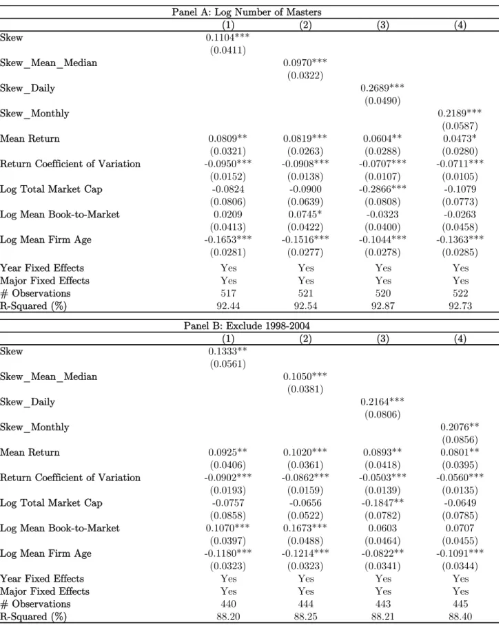
4.8 Robustness Tests
In this section we examine the robustness of our main results in Table 2. We present
these results in Table 11. In Panel A columns (1) – (4), we examine the number of
master’s degree graduates, instead of bachelors. Our results here are very similar to
those in Table 2. In particular, a one-standard-deviation increase in Skew is associated
with a 11% increase in the number of students graduating with a master’s degree in a
related field (column (1)). In columns (2) through (4), we repeat the results presented in
columns (2) through (4) of table 2, but using Master’s degrees, and continue to find
similar results. In unreported results, we have also verified that results remain very
similar if we use data from t-3 to t-6 or from t-3 to t-5. Overall, our result is not specific
to field choice for the bachelor’s degree.
In Panel B, we examine equation (1) again, but we add an additional explanatory
variable, the industry returns moments measured in years (t-1) to (t-2), that is, after
most people have already declared majors. Therefore, it should not have any effect on
major choice. This is what we find, both for Bachelor’s and Master’s degrees. In Panel
C, we continue with this analysis, but now examine entry-level wages and employment.
In the wage regression, we find that higher Skew in years (t-1) to (t-2) is statistically
associated with slightly lower wages, but the economic magnitude of the coefficient is
one-third of that on Skewt-3 to t-7. This possibly reflects that while this skewness is too
recent to elicit major choice decision changes (as shown in columns (5) and (6)), it can
still attract a few graduates from other fields into the entry-level job-market, depressing
wages further. There is no significant association between Skew and entry-level
Finally, in Panel D, we leave out the Tech boom years (1998-2004) from our
analysis, and find similar results, showing that our results do not come solely from
major choices in tech in these periods.
5. Conclusion
This paper examines the effect of superstar firms on an important human capital
decision – college students’ major choice. Intuitively, superstars may play an important
role in shaping college students’ expectations and major choice through two related
channels. First, the occurrences of superstar firms often involve extreme payoffs to the
founders and top executives. Most individuals, in the meanwhile, have a preference for
skewed payoffs, possibly due to the complementarity between taste and income. Second,
superstar firms garner a disproportionate amount of media coverage and social
attention. Given the substantial search frictions faced by college students in choosing
their fields of study, their effort is likely directed by superstar firms.
Using cross-sectional skewness in stock returns or favorable news coverage as
proxies for salient extreme events in an industry, we find that these events are
associated with a disproportionately larger number of college students choosing to major
in related fields. Students’ tendency to follow superstars, however, results in a
temporary over-supply of human capital. In particular, we find that upon entering the
job market, the additional student supply due to salient extreme events lowers the
average wage earned by entry-level employees. Coupled with the finding that the
number of entry-level employees (as well as employee turnover) stays roughly constant,
short run; a sudden increase in labor supply thus lowers the average wage earned by
entry-level employees without affecting the employment size.
In the longer term, firms appear to better cope with the increase in labor supply
by gradually expanding their operations. For example, focusing on positions that require
some prior experience, we find that five years after the extra supply reaching the job
market, there is a significant increase in the number of employees in these advanced
positions in related industries, however at a still depressed wage level.
In sum, our paper is the first to examine the role of salient, extreme events in
determining how people make perhaps the most important and irreversible decision in
their lives – the choice of investment in career skills. Our results have implications for
both labor economists who study the substantial variation in individuals’ education
choice, as well as micro-economists who emphasize the role of salience and skewed
References
Altonji, J. G., 1993, The demand for and return to education when education outcomes are uncertain, Journal of Labor Economics 11, 48-83.
Altonji, J.G., Arcidiacono, P. and Maurel, A., 2015, “The analysis of field choice in college and graduate school: Determinants and wage effects,” National Bureau of Economic Research Working Paper No. 21655.
Altonji, J., Kahn, L. & Speer, J., 2014, “Cashier or consultant? Entry labor market conditions, field of study, and career success,” NBER Working Paper No. 20531.
Altonji, J., Kahn, L. & Speer, J., 2014, “Trends in earnings differentials across college majors and the changing task composition of jobs,” American Economic Review 104(5), 387-93.
Altonji, J., Blom, E. & Meghir, C., 2012, “Heterogeneity in human capital investments: High school curriculum, college major, and careers,” Annual Review of Economics 4, 185-223.
Arcidiacono, P., Hotz, V. J. & Kang, S., 2012, “Modeling college major choices using elicited measures of expectations and counterfactuals,” Journal of Econometrics
166, 3-16.
Arcidiacono, P., Hotz, V., Maurel, A. & Romano, T., 2014, “Recovering ex ante returns and preferences for occupations using subjective expectations data,” NBER Working Paper No. 20626.
Bali, T., N. Cakici, and R. Whitelaw, 2011, “Maxing Out: Stocks as Lotteries and the Cross-section of Expected Returns,” Journal of Financial Economics 99, 427-446.
Beffy, M., Fougere, D. & Maurel, A., 2012, “Choosing the field of studies in postsecondary education: Do expected earnings matter?”'Review of Economics and Statistics 94, 334-347.
Barberis, N. and M. Huang, 2008, “Stocks as Lotteries: The Implications of Probability Weighting for Security Prices,” American Economic Review 98, 2066-2100.
Barberis, N., A. Mukherjee, and B. Wang, 2016, “Prospect theory and stock returns: an empirical test,” Review of Financial Studies, forthcoming.
Berger, M.C., 1988, “Predicted future earnings and choice of college major,” Industrial & Labor Relations Review, 41(3), 418-429.
Bhattacharya, J., 2005, Specialty selection and lifetime returns to specialization', Journal of Human Resources 15, 115-143.
Blom, E., 2012, Labor market determinants of college major, Yale University Working Paper.
Bordon, P., Fu, C., 2015, College-major choice to college-then-major choice, Review of Economic Studies.
Bordalo, P., Gennaioli, N. and Shleifer, A., 2012. “Salience theory of choice under risk,”
Quarterly Journal of Economics 127 (3): 1243 – 1285.
Bordalo, P., Gennaioli, N. and Shleifer, A., 2013a, “Salience and consumer choice,”
Journal of Political Economy 121(5): 803 – 843.
Bordalo, P., Gennaioli, N. and Shleifer, A., 2013b, “Salience and asset prices,” American
Economic Review 103(3), 623-628.
Bordalo, P., Gennaioli, N. and Shleifer, A., 2013c, “Salience theory of judicial decisions,” The Journal of Legal Studies vol. 44(S1), S7 - S33.
Boyer, B., T. Mitton, and K. Vorkink, 2010, “Expected idiosyncratic skewness,” Review of Financial Studies 23, 169-202.
Boyer, B. and K. Vorkink, 2013, “Stock Options as Lotteries,” Journal of Finance, forthcoming.
Chetty, Raj, Adam Looney, and Kory Kroft, 2009, “Salience and Taxation: Theory and Evidence,” American Economic Review 99(4): 1145–77.
Conrad, J., R. Dittmar, and E. Ghysels, 2013, “Ex-Ante Skewness and Expected Stock Returns,” Journal of Finance 68, 85-124.
Dang, T.L., Moshirian, F. and Zhang, B., 2015, “Commonality in News Around the World,” Journal of Financial Economics 116(1), 82-110.
Dickson, L., 2010, “Race and gender differences in college major choice,” The Annals of the American Academy of Political and Social Sciences, 627, 108-124.
Fricke, H., Grogger, J., Steinmayr, A., 2015, Does exposure to economics bring new majors to the field? Evidence from a natural experiment, NBER Working Paper.
Fehr, Ernst, and Antonio Rangel, 2011, “Neuroeconomic Foundations of Economic
Choice — Recent Advances,” Journal of Economic Perspectives 25(4): 3-30.
Gennaioli, N. and Shleifer, A., 2009, “What comes to mind,” Quarterly Journal of Economics 125(4): 1399–1433.
Goldin, C., 2014, “A grand gender convergence: Its last chapter”, American Economic Review 104, 1-30.
Green, T. Clifton, and Byoung-Hyoun Hwang, 2012, “Initial Public Offerings as Lotteries: Skewness Preference and First-Day Returns,” Management Science, 58,
432-444.
Greenwood, R. and Hanson, S.G., 2015, “Waves in ship prices and investment,” The Quarterly Journal of Economics, 55, p.109.
Hastings, J., Neilson, C., Ramirez, A. & Zimmerman, S., “(Un)informed college and major choice: evidence from linked survey and administrative data,” Economics of Education Review, forthcoming.
Hausman, Jerry A., and Gregory K. Leonard, 1997, “Superstars in the National Basketball Association: Economic value and policy,” Journal of Labor Economics 15, no. 4: 586-624.
James, E., Alsalam, N., Conaty, J. C., To, D. L., 1989, “College quality and future earnings: Where should you send your child to college?” American Economic Review 79, 247-252.
Kaldor, Nicholas, 1934, ‘‘A Classificatory Note on the Determination of Equilibrium,’’
Review of Economic Studies, 1, 122–136.
Kumar, A., 2009, “Who Gambles in the Stock Market?” Journal of Finance, 1889-1933.
Lazear, E. P., and Sherwin Rosen, 1981, “Rank-Order Tournaments as Optimum Labor Contracts,” The Journal of Political Economy 89, no. 5: 841-864.
Lemieux, T., 2014, “Occupations, fields of study and returns to education,” Canadian Journal of Economics 47(4), 1-31.
Mitton, T. and K. Vorkink, 2007, “Equilibrium Underdiversification and the Preference for Skewness,” Review of Financial Studies 20, 1255-88.
Pallais, A., 2015, “Small differences that matter: Mistakes in applying to college,”
Rosen, S., 1981, “The economics of superstars,” The American economic review, 71(5), pp.845-858.
Rosen, S, 1997, “Manufactured Inequality,” Journal of Labor Economics 15, no. 2 (1997): 189-196.
Sacerdote, B., 2001, Peer effects with random assignment: Results for Dartmouth roommates, Quarterly Journal of Economics 116, 681-704.
Stigler, George J., 1961, “The economics of information,” Journal of Political Economy. 69 (3): 213–225.
Stigler, George J., 1962, “Information in the labor market,” Journal of Political Economy. 70 (5): 94–105.
Stinebrickner, T. & Stinebrickner, R., 2014, “A major in science? Initial beliefs and final outcomes for college major and dropout,” Review of Economic Studies 81, 426-472.
Taylor, S.E. and Thompson, S.C., 1982, “Stalking the elusive “vividness” effect,”
Psychological review, 89(2), p.155.
Wiswall, M. & Zafar, B., “Determinants of college major choice: identification using an information experiment,”'Review of Economic Studies, forthcoming.
Yuen, J., 2010, “Job-education match and mismatch: Wage differentials,” Perspective on Labour and Income 11, 1-26.