Purely Functional Data Structures - Free Computer, Programming, Mathematics, Technical Books, Lecture Notes and Tutorials

Chris Okasaki

September 1996

CMU-CS-96-177

School of Computer Science Carnegie Mellon University

Pittsburgh, PA 15213

Submitted in partial fulfillment of the requirements for the degree of Doctor of Philosophy.

Thesis Committee: Peter Lee, Chair

Robert Harper Daniel Sleator

Robert Tarjan, Princeton University

Copyright c1996 Chris Okasaki

This research was sponsored by the Advanced Research Projects Agency (ARPA) under Contract No. F19628-95-C-0050.

When a C programmer needs an efficient data structure for a particular prob-lem, he or she can often simply look one up in any of a number of good text-books or handtext-books. Unfortunately, programmers in functional languages such as Standard ML or Haskell do not have this luxury. Although some data struc-tures designed for imperative languages such as C can be quite easily adapted to a functional setting, most cannot, usually because they depend in crucial ways on as-signments, which are disallowed, or at least discouraged, in functional languages. To address this imbalance, we describe several techniques for designing functional data structures, and numerous original data structures based on these techniques, including multiple variations of lists, queues, double-ended queues, and heaps, many supporting more exotic features such as random access or efficient catena-tion.

In addition, we expose the fundamental role of lazy evaluation in amortized functional data structures. Traditional methods of amortization break down when old versions of a data structure, not just the most recent, are available for further processing. This property is known as persistence, and is taken for granted in functional languages. On the surface, persistence and amortization appear to be incompatible, but we show how lazy evaluation can be used to resolve this conflict, yielding amortized data structures that are efficient even when used persistently. Turning this relationship between lazy evaluation and amortization around, the notion of amortization also provides the first practical techniques for analyzing the time requirements of non-trivial lazy programs.

Without the faith and support of my advisor, Peter Lee, I probably wouldn’t even be a graduate student, much less a graduate student on the eve of finishing. Thanks for giving me the freedom to turn my hobby into a thesis.

I am continually amazed by the global nature of modern research and how e-mail allows me to interact as easily with colleagues in Aarhus, Denmark and York, England as with fellow students down the hall. In the case of one such colleague, Gerth Brodal, we have co-authored a paper without ever having met. In fact, sorry Gerth, but I don’t even know how to pronounce your name!

I was extremely fortunate to have had excellent English teachers in high school. Lori Huenink deserves special recognition; her writing and public speaking classes are undoubtedly the most valuable classes I have ever taken, in any subject. In the same vein, I was lucky enough to read my wife’s copy of Lyn Dupr´e’s BUGS in Writing just as I was starting my thesis. If your career involves writing in any form, you owe it to yourself to buy a copy of this book.

Thanks to Maria and Colin for always reminding me that there is more to life than grad school. And to Amy and Mark, for uncountable dinners and other out-ings. We’ll miss you. Special thanks to Amy for reading a draft of this thesis.

Abstract v

Acknowledgments vii

1 Introduction 1

1.1 Functional vs. Imperative Data Structures . . . 1

1.2 Strict vs. Lazy Evaluation . . . 2

1.3 Contributions . . . 3

1.4 Source Language . . . 4

1.5 Terminology . . . 4

1.6 Overview . . . 5

2 Lazy Evaluation and $-Notation 7 2.1 Streams . . . 9

2.2 Historical Notes . . . 10

3 Amortization and Persistence via Lazy Evaluation 13 3.1 Traditional Amortization . . . 13

3.1.1 Example: Queues . . . 15

3.2 Persistence: The Problem of Multiple Futures . . . 19

3.2.1 Execution Traces and Logical Time . . . 19

3.3 Reconciling Amortization and Persistence . . . 20

3.3.1 The Role of Lazy Evaluation . . . 20

3.4 The Banker’s Method . . . 23

3.4.1 Justifying the Banker’s Method . . . 23

3.4.2 Example: Queues . . . 25

3.5 The Physicist’s Method . . . 28

3.5.1 Example: Queues . . . 30

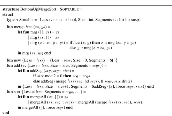
3.5.2 Example: Bottom-Up Mergesort with Sharing . . . 32

3.6 Related Work . . . 37

4 Eliminating Amortization 39 4.1 Scheduling . . . 40

4.2 Real-Time Queues . . . 41

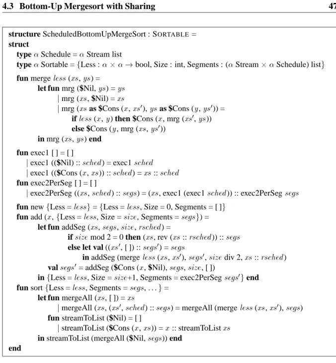
4.3 Bottom-Up Mergesort with Sharing . . . 44

4.4 Related Work . . . 48

5 Lazy Rebuilding 49 5.1 Batched Rebuilding . . . 49

5.2 Global Rebuilding . . . 51

5.3 Lazy Rebuilding . . . 51

5.4 Double-Ended Queues . . . 52

5.4.1 Output-restricted Deques . . . 53

5.4.2 Banker’s Deques . . . 54

5.4.3 Real-Time Deques . . . 57

5.5 Related Work . . . 58

6 Numerical Representations 61 6.1 Positional Number Systems . . . 62

6.2 Binary Representations . . . 64

6.2.1 Binary Random-Access Lists . . . 66

6.2.2 Binomial Heaps . . . 68

6.3 Segmented Binary Numbers . . . 72

6.4 Skew Binary Numbers . . . 76

6.4.1 Skew Binary Random-Access Lists . . . 77

6.4.2 Skew Binomial Heaps . . . 80

6.5 Discussion . . . 82

6.6 Related Work . . . 82

7 Data-Structural Bootstrapping 85 7.1 Structural Decomposition . . . 86

7.1.1 Non-Uniform Recursion and Standard ML . . . 86

7.1.2 Queues Revisited . . . 87

7.2 Structural Abstraction . . . 91

7.2.1 Lists With Efficient Catenation . . . 93

7.2.2 Heaps With Efficient Merging . . . 99

7.3 Related Work . . . 101

8 Implicit Recursive Slowdown 105 8.1 Recursive Slowdown . . . 105

8.2 Implicit Recursive Slowdown . . . 107

8.3 Supporting a Decrement Function . . . 110

8.4 Queues and Deques . . . 112

8.5 Catenable Double-Ended Queues . . . 115

8.6 Related Work . . . 124

9 Conclusions 127 9.1 Functional Programming . . . 127

9.2 Persistent Data Structures . . . 128

9.3 Programming Language Design . . . 128

9.4 Open Problems . . . 130

A The Definition of Lazy Evaluation in Standard ML 131 A.1 Syntax . . . 131

A.2 Static Semantics . . . 132

A.3 Dynamic Semantics . . . 133

Bibliography 137

Introduction

Efficient data structures have been studied extensively for over thirty years, resulting in a vast literature from which the knowledgeable programmer can extract efficient solutions to a stun-ning variety of problems. Much of this literature purports to be language-independent, but unfortunately it is language-independent only in the sense of Henry Ford: Programmers can use any language they want, as long as it’s imperative.1 _{Only a small fraction of existing} data structures are suitable for implementation in functional languages, such as Standard ML or Haskell. This thesis addresses this imbalance by specifically considering the design and analysis of functional data structures.

1.1

Functional vs. Imperative Data Structures

The methodological benefits of functional languages are well known [Bac78, Hug89, HJ94], but still the vast majority of programs are written in imperative languages such as C. This apparent contradiction is easily explained by the fact that functional languages have historically been slower than their more traditional cousins, but this gap is narrowing. Impressive advances have been made across a wide front, from basic compiler technology to sophisticated analyses and optimizations. However, there is one aspect of functional programming that no amount of cleverness on the part of the compiler writer is likely to mitigate — the use of inferior or inappropriate data structures. Unfortunately, the existing literature has relatively little advice to offer on this subject.

Why should functional data structures be any more difficult to design and implement than imperative ones? There are two basic problems. First, from the point of view of designing and implementing efficient data structures, functional programming’s stricture against destructive

1_{Henry Ford once said of the available colors for his Model T automobile, “[Customers] can have any color}

updates (assignments) is a staggering handicap, tantamount to confiscating a master chef’s knives. Like knives, destructive updates can be dangerous when misused, but tremendously effective when used properly. Imperative data structures often rely on assignments in crucial ways, and so different solutions must be found for functional programs.

The second difficulty is that functional data structures are expected to be more flexible than their imperative counterparts. In particular, when we update an imperative data structure we typically accept that the old version of the data structure will no longer be available, but, when we update a functional data structure, we expect that both the old and new versions of the data structure will be available for further processing. A data structure that supports multiple versions is called persistent while a data structure that allows only a single version at a time is called ephemeral [DSST89]. Functional programming languages have the curious property that all data structures are automatically persistent. Imperative data structures are typically ephemeral, but when a persistent data structure is required, imperative programmers are not surprised if the persistent data structure is more complicated and perhaps even asymptotically less efficient than an equivalent ephemeral data structure.

Furthermore, theoreticians have established lower bounds suggesting that functional pro-gramming languages may be fundamentally less efficient than imperative languages in some situations [BAG92, Pip96]. In spite of all these points, this thesis shows that it is often possible to devise functional data structures that are asymptotically as efficient as the best imperative solutions.

1.2

Strict vs. Lazy Evaluation

Most (sequential) functional programming languages can be classified as either strict or lazy, according to their order of evaluation. Which is superior is a topic debated with religious fervor by functional programmers. The difference between the two evaluation orders is most apparent in their treatment of arguments to functions. In strict languages, the arguments to a function are evaluated before the body of the function. In lazy languages, arguments are evaluated in a demand-driven fashion; they are initially passed in unevaluated form and are evaluated only when (and if!) the computation needs the results to continue. Furthermore, once a given argument is evaluated, the value of that argument is cached so that if it is ever needed again, it can be looked up rather than recomputed. This caching is known as memoization [Mic68].

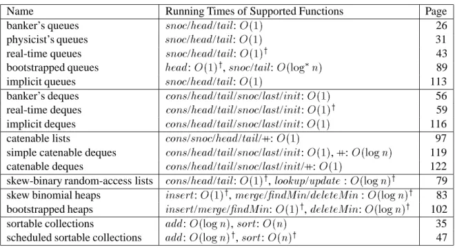
Name Running Times of Supported Functions Page

banker’s queues

snoc

/

head

/

tail

:O (1) 26

physicist’s queues

snoc

/

head

/

tail

:O (1) 31

real-time queues

snoc

/

head

/

tail

:O (1) y

43 bootstrapped queues

head

:O (1)

y

,

snoc

/

tail

:O (log

n) 89

implicit queues

snoc

/

head

/

tail

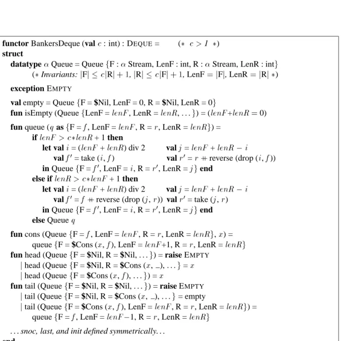
:O (1) 113

banker’s deques

cons

/

head

/

tail

/

snoc

/

last

/

init

:O (1) 56 real-time deques

cons

/

head

/

tail

/

snoc

/

last

/

init

:O (1)

y

59 implicit deques

cons

/

head

/

tail

/

snoc

/

last

/

init

:O (1) 116 catenable lists

cons

/

snoc

/

head

/

tail

/++:O (1) 97 simple catenable deques

cons

/

head

/

tail

/

snoc

/

last

/

init

:O (1), ++:O (logn) 119 catenable deques

cons

/

head

/

tail

/

snoc

/

last

/

init

/++:O (1) 122 skew-binary random-access lists

cons

/

head

/

tail

:O (1)

y

,

lookup

/

update

:O (logn) y

79 skew binomial heaps

insert

:O (1)

y

,

merge

/

ndMin

/

deleteMin

:O (logn) y

83 bootstrapped heaps

insert

/

merge

/

ndMin

:O (1)

y

,

deleteMin

:O (logn) y

102 sortable collections

add

:O (logn),

sort

:O (n) 35 scheduled sortable collections

add

:O (logn)

y

,

sort

:O (n) y

47 Worst-case running times marked withy. All other running times are amortized.

Table 1.1: Summary of Implementations

are often reduced to pretending the language is actually strict to make even gross estimates of running time!

Both evaluation orders have implications for the design and analysis of data structures. As we will see in Chapters 3 and 4, strict languages can describe worst-case data structures, but not amortized ones, and lazy languages can describe amortized data structures, but not worst-case ones. To be able to describe both kinds of data structures, we need a programming language that supports both evaluation orders. Fortunately, combining strict and lazy evaluation in a single language is not difficult. Chapter 2 describes $-notation — a convenient way of adding lazy evaluation to an otherwise strict language (in this case, Standard ML).

1.3

Contributions

This thesis makes contributions in three major areas:

Functional programming. Besides developing a suite of efficient data structures that

designing and analyzing functional data structures, including powerful new techniques for reasoning about the running time of lazy programs.

Persistent data structures. Until this research, it was widely believed that amortization

was incompatible with persistence [DST94, Ram92]. However, we show that memoiza-tion, in the form of lazy evaluamemoiza-tion, is the key to reconciling the two. Furthermore, as noted by Kaplan and Tarjan [KT96b], functional programming is a convenient medium for developing new persistent data structures, even when the data structure will eventu-ally be implemented in an imperative language. The data structures and techniques in this thesis can easily be adapted to imperative languages for those situations when an imperative programmer needs a persistent data structure.

Programming language design. Functional programmers have long debated the relative

merits of strict and lazy evaluation. This thesis shows that both are algorithmically im-portant and suggests that the ideal functional language should seamlessly integrate both. As a modest step in this direction, we propose $-notation, which allows the use of lazy evaluation in a strict language with a minimum of syntactic overhead.

1.4

Source Language

All source code will be presented in Standard ML [MTH90], extended with primitives for lazy evaluation. However, the algorithms can all easily be translated into any other functional language supporting both strict and lazy evaluation. Programmers in functional languages that are either entirely strict or entirely lazy will be able to use some, but not all, of the data structures in this thesis.

In Chapters 7 and 8, we will encounter several recursive data structures that are difficult to describe cleanly in Standard ML because of the language’s restrictions against certain sophisti-cated and difficult-to-implement forms of recursion, such as polymorphic recursion and recur-sive modules. When this occurs, we will first sacrifice executability for clarity and describe the data structures using ML-like pseudo-code incorporating the desired forms of recursion. Then, we will show how to convert the given implementations to legal Standard ML. These examples should be regarded as challenges to the language design community to provide a programming language capable of economically describing the appropriate abstractions.

1.5

Terminology

An abstract data type (that is, a type and a collection of functions on that type). We will

refer to this as an abstraction.

A concrete realization of an abstract data type. We will refer to this as an

implementa-tion, but note that an implementation need not be actualized as code — a concrete design is sufficient.

An instance of a data type, such as a particular list or tree. We will refer to such an

instance generically as an object or a version. However, particular data types typically have their own nomenclature. For example, we will refer to stack or queue objects simply as stacks or queues.

A unique identity that is invariant under updates. For example, in a stack-based

in-terpreter, we often speak informally about “the stack” as if there were only one stack, rather than different versions at different times. We will refer to this identity as a persis-tent identity. This issue mainly arises in the context of persispersis-tent data structures; when we speak of different versions of the same data structure, we mean that the different versions share a common persistent identity.

Roughly speaking, abstractions correspond to signatures in Standard ML, implementations to structures or functors, and objects or versions to values. There is no good analogue for persistent identities in Standard ML.2

The term operation is similarly overloaded, meaning both the functions supplied by an abstract data type and applications of those functions. We reserve the term operation for the latter meaning, and use the terms operator or function for the former.

1.6

Overview

This thesis is structured in two parts. The first part (Chapters 2–4) concerns algorithmic aspects of lazy evaluation. Chapter 2 sets the stage by briefly reviewing the basic concepts of lazy evaluation and introducing $-notation.

Chapter 3 is the foundation upon which the rest of the thesis is built. It describes the mediating role lazy evaluation plays in combining amortization and persistence, and gives two methods for analyzing the amortized cost of data structures implemented with lazy evaluation. Chapter 4 illustrates the power of combining strict and lazy evaluation in a single language. It describes how one can often derive a worst-case data structure from an amortized data struc-ture by systematically scheduling the premastruc-ture execution of lazy components.

2_{The persistent identity of an ephemeral data structure can be reified as a reference cell, but this is insufficient}

The second part of the thesis (Chapters 5–8) concerns the design of functional data struc-tures. Rather than cataloguing efficient data structures for every purpose (a hopeless task!), we instead concentrate on a handful of general techniques for designing efficient functional data structures and illustrate each technique with one or more implementations of fundamental ab-stractions such as priority queues, random-access structures, and various flavors of sequences. Chapter 5 describes lazy rebuilding, a lazy variant of global rebuilding [Ove83]. Lazy re-building is significantly simpler than global rere-building, but yields amortized rather than worst-case bounds. By combining lazy rebuilding with the scheduling techniques of Chapter 4, the worst-case bounds can be recovered.

Chapter 6 explores numerical representations, implementations designed in analogy to rep-resentations of numbers (typically binary numbers). In this model, designing efficient insertion and deletion routines corresponds to choosing variants of binary numbers in which adding or subtracting one take constant time.

Chapter 7 examines data-structural bootstrapping [Buc93]. Data-structural bootstrapping comes in two flavors: structural decomposition, in which unbounded solutions are bootstrapped from bounded solutions, and structural abstraction, in which efficient solutions are boot-strapped from inefficient solutions.

Chapter 8 describes implicit recursive slowdown, a lazy variant of the recursive-slowdown technique of Kaplan and Tarjan [KT95]. As with lazy rebuilding, implicit recursive slowdown is significantly simpler than recursive slowdown, but yields amortized rather than worst-case bounds. Again, we can recover the worst-case bounds using scheduling.

Lazy Evaluation and $-Notation

Lazy evaluation is an evaluation strategy employed by many purely functional programming languages, such as Haskell [H+

92]. This strategy has two essential properties. First, the evalu-ation of a given expression is delayed, or suspended, until its result is needed. Second, the first time a suspended expression is evaluated, the result is memoized (i.e., cached) so that the next time it is needed, it can be looked up rather than recomputed.

Supporting lazy evaluation in a strict language such as Standard ML requires two primi-tives: one to suspend the evaluation of an expression and one to resume the evaluation of a suspended expression (and memoize the result). These primitives are often called

delay

and

force

. For example, Standard ML of New Jersey offers the following primitives for lazy eval-uation:

type

susp

val delay : (unit!

)!

susp

val force :

susp!

These primitives are sufficient to encode all the algorithms in this thesis. However, program-ming with these primitives can be rather inconvenient. For instance, to suspend the evaluation of some expression

e

, one writes

delay

(

fn

())

e

). Depending on the use of whitespace, this

introduces an overhead of 13–17 characters! Although acceptable when only a few expressions are to be suspended, this overhead quickly becomes intolerable when many expressions must be delayed.

If

s

is a suspension of type

susp

, then

force

s

evaluates and memoizes the contents of

s

and returns the resulting value of type

. However, explicitly forcing a suspension with a

force

operation can also be inconvenient. In particular, it often interacts poorly with pattern matching, requiring a single

case

expression to be broken into two or more nested

case

ex-pressions, interspersed with

force

operations. To avoid this problem, we integrate $-notation with pattern matching. Matching a suspension against a pattern of the form $

p

first forces the suspension and then matches the result against

p

. At times, an explicit

force

operator is still useful. However, it can now be defined in terms of $ patterns.

fun force ($

x

) =

x

To compare the two notations, consider the standard

take

function, which extracts the first

n

elements of a stream. Streams are defined as follows:

datatype

StreamCell = NiljCons of

Stream

withtype

Stream =

StreamCell susp Using

delay

and

force

,

take

would be written

fun take (

n

,

s

) =

delay (fn ())case

n

of

0)Nil

j )case force

s

of

Nil)Nil jCons (

x

,

s

0

))Cons (

x

, take (

n

;1,

s

0

))) In contrast, using $-notation,

take

can be written more concisely as

fun take (

n

,

s

) = $case (

n

,

s

) of (0, ))Nil j( , $Nil))Nil j( , $Cons (

x

,

s

0

)))Cons (

x

, take (

n

;1,

s

0

)) In fact, it is tempting to write

take

even more concisely as

fun take (0, ) = $Nil

jtake ( , $Nil) = $Nil

jtake (

n

, $Cons (

x

,

s

)) = $Cons (

x

, take (

n

;1,

s

))

However, this third implementation is not equivalent to the first two. In particular, it forces its second argument when

take

is applied, rather than when the resulting stream is forced.

2.1

Streams

As an extended example of lazy evaluation and $-notation in Standard ML, we next develop a small streams package. These streams will also be used by several of the data structures in subsequent chapters.

Streams (also known as lazy lists) are very similar to ordinary lists, except that every cell is systematically suspended. The type of streams is

datatype

StreamCell = NiljCons of

Stream

withtype

Stream =

StreamCell susp

A simple stream containing the elements 1, 2, and 3 could be written $Cons (1, $Cons (2, $Cons (3, $Nil)))

It is illuminating to contrast streams with simple suspended lists of type

list susp

. The computations represented by the latter type are inherently monolithic — once begun by forcing the suspended list, they run to completion. The computations represented by streams, on the other hand, are often incremental — forcing a stream executes only enough of the computation to produce the outermost cell and suspends the rest. This behavior is common among datatypes such as streams that contain nested suspensions.

To see this difference in behavior more clearly, consider the append function, written

s

++

t

. On suspended lists, this function might be written fun

s

++

t

= $(force

s

@ force

t

)

Once begun, this function forces both its arguments and then appends the two lists, producing the entire result. Hence, this function is monolithic. On streams, the append function is written

fun

s

++

t

= $case

s

of

$Nil)force

t

j$Cons (

x

,

s

0

))Cons (

x

,

s

0

++

t

)

Once begun, this function forces the first cell of

s

(by matching against a $ pattern). If this cell is

Nil

, then the first cell of the result is the first cell of

t

, so the function forces

t

. Otherwise, the function constructs the first cell of the result from the first element of

s

and — this is the key point — the suspension that will eventually calculate the rest of the appended list. Hence, this function is incremental. The

take

function described earlier is similarly incremental.

However, consider the function to drop the first

n

elements of a stream. fun drop (

n

,

s

) = let fun drop0

(0,

s

0

) = force

s

0 jdrop

0

jdrop 0

(

n

, $Cons (

x

,

s

0

)) = drop0

(

n

;1,

s

0

) in $drop0

(

n

,

s

) end

This function is monolithic because the recursive calls to

drop

0

are never delayed — calcu-lating the first cell of the result requires executing the entire drop function. Another common monolithic stream function is

reverse

.

fun reverse

s

= let fun reverse0

($Nil,

r

) =

r

jreverse 0

($Cons (

x

,

s

),

r

) = reverse0

(

s

, Cons (

x

, $

r

)) in $reverse0

(

s

, Nil) end Here the recursive calls to

reverse

0

are never delayed, but note that each recursive call creates a new suspension of the form $

r

. It might seem then that

reverse

does not in fact do all of its work at once. However, suspensions such as these, whose bodies are manifestly values (i.e., composed entirely of constructors and variables, with no function applications), are called trivial. A good compiler would create these suspensions in already-memoized form, but even if the compiler does not perform this optimization, trivial suspensions always evaluate in

O(1)

time.

Although monolithic stream functions such as

drop

and

reverse

are common, incremental functions such as ++ and

take

are the raison d’ˆetre of streams. Each suspension carries a small but significant overhead, so for maximum efficiency laziness should be used only when there is a good reason to do so. If the only uses of lazy lists in a given application are monolithic, then that application should use simple suspended lists rather than streams.

Figure 2.1 summarizes these stream functions as a Standard ML module. Note that the type of streams is defined using Standard ML’s

withtype

construction, but that older versions of Standard ML do not allow

withtype

declarations in signatures. This feature will be sup-ported in future versions of Standard ML, but if your compiler does not allow it, then a sim-ple workaround is to delete the

Stream

type and replace every occurrence of

Stream

with

StreamCell susp

. By including the

StreamCell

datatype in the signature, we have delib-erately chosen to expose the internal representation in order to support pattern matching on streams.

2.2

Historical Notes

Lazy Evaluation Wadsworth [Wad71] first proposed lazy evaluation as an optimization of normal-order reduction in the lambda calculus. Vuillemin [Vui74] later showed that, under certain restricted conditions, lazy evaluation is an optimal evaluation strategy. The formal semantics of lazy evaluation has been studied extensively [Jos89, Lau93, OLT94, AFM+

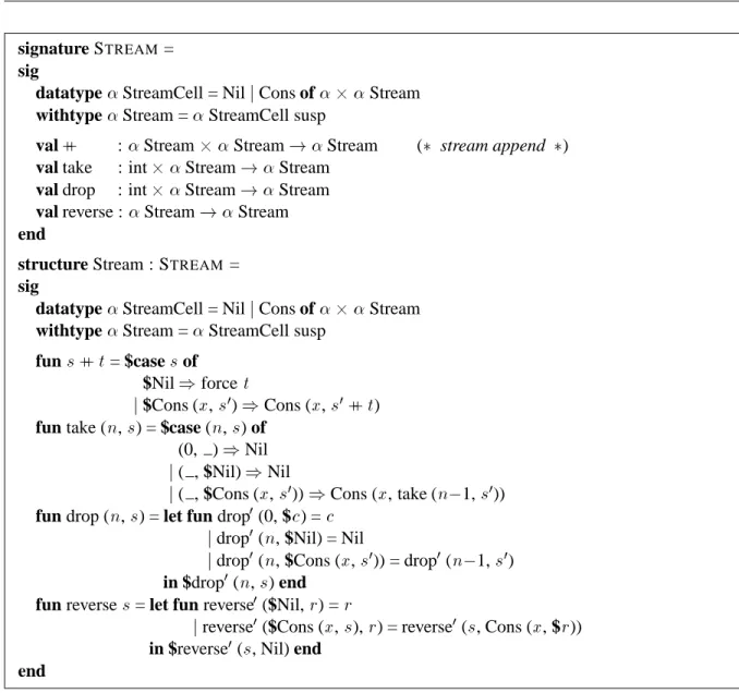
signature STREAM=

sig

datatypeStreamCell = NiljCons ofStream

withtypeStream =StreamCell susp

val ++ :StreamStream!Stream ( stream append )

val take : intStream!Stream

val drop : intStream!Stream

val reverse : Stream!Stream

end

structure Stream : STREAM=

sig

datatypeStreamCell = NiljCons ofStream

withtypeStream =StreamCell susp

fun

s

++

t

= $case

s

of $Nil)force

t

j$Cons (

x

,

s

0

))Cons (

x

,

s

0

++

t

)

fun take (

n

,

s

) = $case (

n

,

s

) of (0, ))Nil j( , $Nil))Nil j( , $Cons (

x

,

s

0

)))Cons (

x

, take (

n

;1,

s

0

))

fun drop (

n

,

s

) = let fun drop0

(0, $

c

) =

c

jdrop

0

(

n

, $Nil) = Nil jdrop

0

(

n

, $Cons (

x

,

s

0

)) = drop0

(

n

;1,

s

0

)

in $drop0

(

n

,

s

) end

fun reverse

s

= let fun reverse0

($Nil,

r

) =

r

jreverse

0

($Cons (

x

,

s

),

r

) = reverse0

(

s

, Cons (

x

, $

r

))

in $reverse0

(

s

, Nil) end

end

Figure 2.1: A small streams package.

Streams Landin introduced streams in [Lan65], but without memoization. Friedman and Wise [FW76] and Henderson and Morris [HM76] extended Landin’s streams with memoiza-tion.

memoization, in the original sense of Michie, to functional programs.

Algorithmics Both components of lazy evaluation — delaying computations and memoizing the results — have a long history in algorithm design, although not always in combination. The idea of delaying the execution of potentially expensive computations (often deletions) is used to good effect in hash tables [WV86], priority queues [ST86b, FT87], and search trees [DSST89]. Memoization, on the other hand, is the basic principle of such techniques as dynamic program-ming [Bel57] and path compression [HU73, TvL84].

Syntax for Lazy Evaluation Early versions of CAML [W+

Amortization and Persistence via Lazy

Evaluation

Over the past fifteen years, amortization has become a powerful tool in the design and analysis of data structures. Implementations with good amortized bounds are often simpler and faster than implementations with equivalent worst-case bounds. Unfortunately, standard techniques for amortization apply only to ephemeral data structures, and so are unsuitable for designing or analyzing functional data structures, which are automatically persistent.

In this chapter, we review the two traditional techniques for analyzing amortized data struc-tures — the banker’s method and the physicist’s method — and show where they break down for persistent data structures. Then, we demonstrate how lazy evaluation can mediate the con-flict between amortization and persistence. Finally, we adapt the banker’s and physicist’s meth-ods to analyze lazy amortized data structures.

The resulting techniques are both the first techniques for designing and analyzing persis-tent amortized data structures and the first practical techniques for analyzing non-trivial lazy programs.

3.1

Traditional Amortization

up a wide design space of possible solutions, and often yields new solutions that are simpler and faster than worst-case solutions with equivalent bounds. In fact, for some problems, such as the union-find problem [TvL84], there are amortized solutions that are asymptotically faster than any possible worst-case solution (assuming certain modest restrictions) [Blu86].

To prove an amortized bound, one defines the amortized cost of each operation and then proves that, for any sequence of operations, the total amortized cost of the operations is an upper bound on the total actual cost, i.e.,

m

X

i=1

a

i

m

X

i=1

t

i

where

a

i is the amortized cost of operation

i

,

t

i is the actual cost of operation

i

, and

m

is the total number of operations. Usually, in fact, one proves a slightly stronger result: that at any intermediate stage in a sequence of operations, the accumulated amortized cost is an upper bound on the accumulated actual cost, i.e.,

j

X

i=1

a

i

j

X

i=1

t

i

for any

j

. The difference between the accumulated amortized costs and the accumulated actual costs is called the accumulated savings. Thus, the accumulated amortized costs are an upper bound on the accumulated actual costs whenever the accumulated savings is non-negative.

Amortization allows for occasional operations to have actual costs that exceed their amor-tized costs. Such operations are called expensive. Operations whose actual costs are less than their amortized costs are called cheap. Expensive operations decrease the accumulated savings and cheap operations increase it. The key to proving amortized bounds is to show that expen-sive operations occur only when the accumulated savings are sufficient to cover the cost, since otherwise the accumulated savings would become negative.

Tarjan [Tar85] describes two techniques for analyzing ephemeral amortized data structures: the banker’s method and the physicist’s method. In the banker’s method, the accumulated sav-ings are represented as credits that are associated with individual locations in the data structure. These credits are used to pay for future accesses to these locations. The amortized cost of any operation is defined to be the actual cost of the operation plus the credits allocated by the operation minus the credits spent by the operation, i.e.,

a

i

=

t

i

+

c

i;

c

i

where

c

i is the number of credits allocated by operation

i

, and

c

i is the number of credits spent by operation

i

. Every credit must be allocated before it is spent, and no credit may be spent more than once. Therefore, P

c

i P

c

i, which in turn guarantees thatP

a

i P

t

i,

the distribution of credits in such a way that, whenever an expensive operation might occur, sufficient credits have been allocated in the right locations to cover its cost.

In the physicist’s method, one describes a function

that maps each object

d

to a real number called the potential of

d

. The function

is typically chosen so that the potential is initially zero and is always non-negative. Then, the potential represents a lower bound on the accumulated savings.

Let

d

i be the output of operation

i

and the input of operation

i+1

. Then, the amortized cost of operation

i

is defined to be the actual cost plus the change in potential between

d

i;1and

d

i,

i.e.,

a

i

=

t

i

+ (d

i

)

;

(d

i ;1

)

The accumulated actual costs of the sequence of operations are

Pj

i=1

t

i

=

Pj

i=1

(a

i

+ (d

i ;1

)

;

(d

i

))

=

Pj

i=1

a

i

+

Pj

i=1

((d

i ;1

)

;

(d

i

))

=

Pj

i=1

a

i

+ (d

0

)

;

(d

j

)

Sums such asP

((d

i;1

)

;

(d

i

))

, where alternating positive and negative terms cancel each

other out, are called telescoping series. Provided

is chosen in such a way that

(d

0

)

is zero

and

(d

j

)

is non-negative, then

(d

j

)

(d

0

)

and

P

a

i P

t

i, so the accumulated amortized

costs are an upper bound on the accumulated actual costs, as desired.

Remark: This is a somewhat simplified view of the physicist’s method. In real analyses, one often encounters situations that are difficult to fit into the framework as described. For example, what about functions that take or return more than one object? However, this simplified view

suffices to illustrate the relevant issues. 3

Clearly, the two methods are very similar. We can convert the banker’s method to the physi-cist’s method by ignoring locations and taking the potential to be the total number of credits in the object, as indicated by the credit invariant. Similarly, we can convert the physicist’s method to the banker’s method by converting potential to credits, and placing all credits on the root. It is perhaps surprising that the knowledge of locations in the banker’s method offers no extra power, but the two methods are in fact equivalent [Tar85, Sch92]. The physicist’s method is usually simpler, but it is occasionally convenient to take locations into account.

Note that both credits and potential are analysis tools only; neither actually appears in the program text (except maybe in comments).

3.1.1

Example: Queues

signature QUEUE=

sig

typeQueue

exception EMPTY

val empty :Queue

val isEmpty :Queue!bool

val snoc :Queue!Queue

val head :Queue! (raises EMPTYif queue is empty)

val tail :Queue!Queue (raises EMPTYif queue is empty)

end

Figure 3.1: Signature for queues.

(Etymological note:

snoc

is

cons

spelled backward and means “cons on the right”.)

A common representation for purely functional queues [Gri81, HM81, Bur82] is as a pair of lists,

F

and

R

, where

F

contains the front elements of the queue in the correct order and

R

contains the rear elements of the queue in reverse order. For example, a queue containing the integers 1. . . 6 might be represented by the lists

F

= [1,2,3] and

R

= [6,5,4]. This representation is described by the following datatype:

datatype

Queue = Queue offF :

list, R :

listg

In this representation, the head of the queue is the first element of

F

, so

head

and

tail

return and remove this element, respectively.

fun head (QueuefF =

x

::

f

, R =

r

g) =

x

fun tail (QueuefF =

x

::

f

, R =

r

g) = QueuefF =

f

, R =

r

g

Remark: To avoid distracting the reader with minor details, we will commonly ignore error cases when presenting code fragments. For example, the above code fragments do not describe the behavior of

head

or

tail

on empty queues. We will always include the error cases when

presenting complete implementations. 3

Now, the last element of the queue is the first element of

R

, so

snoc

simply adds a new element at the head of

R

.

Elements are added to

R

and removed from

F

, so they must somehow migrate from one list to the other. This is accomplished by reversing

R

and installing the result as the new

F

whenever

F

would otherwise become empty, simultaneously setting the new

R

to [ ]. The goal is to maintain the invariant that

F

is empty only if

R

is also empty (i.e., the entire queue is empty). Note that if

F

were empty when

R

was not, then the first element of the queue would be the last element of

R

, which would take

O(n)

time to access. By maintaining this invariant, we guarantee that

head

can always find the first element in

O(1)

time.

snoc

and

tail

must now detect those cases that would otherwise result in a violation of the invariant, and change their behavior accordingly.

fun snoc (QueuefF = [ ], . . .g,

x

) = QueuefF = [

x

], R = [ ]g jsnoc (QueuefF =

f

, R =

r

g,

x

) = QueuefF =

f

, R =

x

::

r

g

fun tail (QueuefF = [

x

], R =

r

g) = QueuefF = rev

r

, R = [ ]g jtail (QueuefF =

x

::

f

, R =

r

g) = QueuefF =

f

, R =

r

g

Note the use of the record wildcard (. . . ) in the first clause of

snoc

. This is Standard ML pattern-matching notation meaning “the remaining fields of this record are irrelevant”. In this case, the

R

field is irrelevant because we know by the invariant that if

F

is [ ], then so is

R

.

A cleaner way to write these functions is to consolidate the invariant-maintenance duties of

snoc

and

tail

into a single pseudo-constructor. Pseudo-constructors, sometimes called smart constructors [Ada93], are functions that replace ordinary constructors in the construction of data, but that check and enforce an invariant. In this case, the pseudo-constructor

queue

re-places the ordinary constructor

Queue

, but guarantees that

F

is empty only if

R

is also empty.

fun queuefF = [ ], R =

r

g= QueuefF = rev

r

, R = [ ]g jqueuefF =

f

, R =

r

g= QueuefF =

f

, R =

r

g

fun snoc (QueuefF =

f

, R =

r

g,

x

) = queuefF =

f

, R =

x

::

r

g

fun tail (QueuefF =

x

::

f

, R =

r

g) = queuefF =

f

, R =

r

g

The complete code for this implementation is shown in Figure 3.2. Every function except

tail

takes

O(1)

worst-case time, but

tail

takes

O(n)

worst-case time. However, we can show that

snoc

and

tail

each take only

O(1)

amortized time using either the banker’s method or the physicist’s method.

structure BatchedQueue : QUEUE=

struct

datatypeQueue = Queue offF :list, R :listg (Invariant: F is empty only if R is also empty)

exception EMPTY

val empty = QueuefF = [ ], R = [ ]g

fun isEmpty (QueuefF =

f

, R =

r

g) = null

f

fun queuefF = [ ], R =

r

) = QueuefF = rev

r

, R = [ ]g jqueue

q

= Queue

q

fun snoc (QueuefF =

f

, R =

r

),

x

) = queuefF =

f

, R =

x

::

r

g

fun head (QueuefF = [ ], . . .g) = raise EMPTY jhead (QueuefF =

x

::

f

, . . .g) =

x

fun tail (QueuefF = [ ], . . .g) = raise EMPTY

jtail (QueuefF =

x

::

f

, R =

r

g) = queuefF =

f

, R =

r

g

end

Figure 3.2: A common implementation of purely functional queues [Gri81, HM81, Bur82].

Using the physicist’s method, we define the potential function

to be the length of the rear list. Then every

snoc

into a non-empty queue takes one actual step and increases the potential by one, for an amortized cost of two. Every

tail

that does not reverse the rear list takes one actual step and leaves the potential unchanged, for an amortized cost of one. Finally, every

tail

that does reverse the rear list takes

m+1

actual steps and sets the new rear list to [ ], decreasing the potential by

m

, for an amortized cost of

m + 1

;

m = 1

.

3.2

Persistence: The Problem of Multiple Futures

In the above analyses, we implicitly assumed that queues were used ephemerally (i.e., in a single-threaded fashion). What happens if we try to use these queues persistently?

Let

q

be the result of inserting

n

elements into an initially empty queue, so that the front list of

q

contains a single element and the rear list contains

n

;

1

elements. Now, suppose

we use

q

persistently by taking its tail

n

times. Each call of

tail q

takes

n

actual steps. The total actual cost of this sequence of operations, including the time to build

q

, is

n

2

+

n

. If the operations truly took

O(1)

amortized time each, then the total actual cost would be only

O(n)

. Clearly, using these queues persistently invalidates the

O(1)

amortized time bounds proved above. Where do these proofs go wrong?

In both cases, a fundamental requirement of the analysis is violated by persistent data struc-tures. The banker’s method requires that no credit be spent more than once, while the physi-cist’s method requires that the output of one operation be the input of the next operation (or, more generally, that no output be used as input more than once). Now, consider the second call to

tail q

in the example above. The first call to

tail q

spends all the credits on the rear list of

q

, leaving none to pay for the second and subsequent calls, so the banker’s method breaks. And the second call to

tail q

reuses

q

rather than the output of the first call, so the physicist’s method breaks.

Both these failures reflect the inherent weakness of any accounting system based on ac-cumulated savings — that savings can only be spent once. The traditional methods of amor-tization operate by accumulating savings (as either credits or potential) for future use. This works well in an ephemeral setting, where every operation has only a single logical future. But with persistence, an operation might have multiple logical futures, each competing to spend the same savings.

3.2.1

Execution Traces and Logical Time

What exactly do we mean by the “logical future” of an operation?

We model logical time with execution traces, which give an abstract view of the history of a computation. An execution trace is a directed graph whose nodes represent “interesting” operations, usually just update operations on the data type in question. An edge from

v

to

v

0

indicates that operation

v

0

futures. We will sometimes refer to the logical history or logical future of an object, meaning the logical history or logical future of the operation that created the object.

Execution traces generalize the notion of version graphs [DSST89], which are often used to model the histories of persistent data structures. In a version graph, nodes represent the various versions of a single persistent identity and edges represent dependencies between versions. Thus, version graphs model the results of operations and execution traces model the operations themselves. Execution traces are often more convenient for combining the histories of several persistent identities (perhaps not even of the same data type) or for reasoning about operations that do not return a new version (e.g., queries) or that return several results (e.g., splitting a list into two sublists).

For ephemeral data structures, the out-degree of every node in a version graph or execu-tion trace is typically restricted to be at most one, reflecting the limitaexecu-tion that objects can be updated at most once. To model various flavors of persistence, version graphs allow the out-degree of every node to be unbounded, but make other restrictions. For instance, version graphs are often limited to be trees (forests) by restricting the in-degree of every node to be at most one. Other version graphs allow in-degrees of greater than one, but forbid cycles, making every graph a dag. We make none of these restrictions on execution traces. Nodes with in-degree greater than one correspond to operations that take more than one argument, such as list catenation or set union. Cycles arise from recursively defined objects, which are supported by many lazy languages. We even allow multiple edges between a single pair of nodes, as might occur if a list is catenated with itself.

We will use execution traces in Section 3.4.1 when we extend the banker’s method to cope with persistence.

3.3

Reconciling Amortization and Persistence

In the previous section, we saw that traditional methods of amortization break in the presence of persistence because they assume a unique future, in which the accumulated savings will be spent at most once. However, with persistence, multiple logical futures might all try to spend the same savings. In this section, we show how the banker’s and physicist’s methods can be repaired by replacing the notion of accumulated savings with accumulated debt, where debt measures the cost of unevaluated lazy computations. The intuition is that, although savings can only be spent once, it does no harm to pay off debt more than once.

3.3.1

The Role of Lazy Evaluation

malicious adversary might call

f x

arbitrarily often. (Note that each operation is a new logi-cal future of

x

.) If each operation takes the same amount of time, then the amortized bounds degrade to the worst-case bounds. Hence, we must find a way to guarantee that if the first application of

f

to

x

is expensive, then subsequent applications of

f

to

x

will not be.

Without side-effects, this is impossible under by-value (i.e., strict evaluation) or call-by-name (i.e., lazy evaluation without memoization), because every application of

f

to

x

will take exactly the same amount of time. Therefore, amortization cannot be usefully combined with persistence in languages supporting only these evaluation orders.

But now consider call-by-need (i.e., lazy evaluation with memoization). If

x

contains some suspended component that is needed by

f

, then the first application of

f

to

x

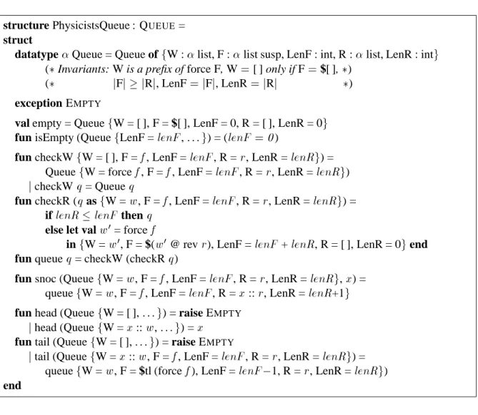
will force the (potentially expensive) evaluation of that component and memoize the result. Subsequent op-erations may then access the memoized result directly. This is exactly the desired behavior! Remark: In retrospect, the relationship between lazy evaluation and amortization is not surprising. Lazy evaluation can be viewed as a form of self-modification, and amortization often involves self-modification [ST85, ST86b]. However, lazy evaluation is a particularly disciplined form of self-modification — not all forms of self-modification typically used in amortized ephemeral data structures can be encoded as lazy evaluation. In particular, splay-ing [ST85] does not appear to be amenable to this technique. 3

3.3.2

A Framework for Analyzing Lazy Data Structures

We have just shown that lazy evaluation is necessary to implement amortized data structures purely functionally. Unfortunately, analyzing the running times of programs involving lazy evaluation is notoriously difficult. Historically, the most common technique for analyzing lazy programs has been to pretend that they are actually strict. However, this technique is completely inadequate for analyzing lazy amortized data structures. We next describe a basic framework to support such analyses. In the remainder of this chapter, we will adapt the banker’s and physicist’s methods to this framework, yielding both the first techniques for analyzing persistent amortized data structures and the first practical techniques for analyzing non-trivial lazy programs.

the sum of its shared and unshared costs. Note that the complete cost is what the actual cost of the operation would be if lazy evaluation were replaced with strict evaluation.

We further partition the total shared costs of a sequence of operations into realized and unrealized costs. Realized costs are the shared costs for suspensions that are executed during the overall computation. Unrealized costs are the shared costs for suspensions that are never executed. The total actual cost of a sequence of operations is the sum of the unshared costs and the realized shared costs — unrealized costs do not contribute to the actual cost. Note that the amount that any particular operation contributes to the total actual cost is at least its unshared cost, and at most its complete cost, depending on how much of its shared cost is realized.

We account for shared costs using the notion of accumulated debt. Initially, the accumu-lated debt is zero, but every time a suspension is created, we increase the accumuaccumu-lated debt by the shared cost of the suspension (and any nested suspensions). Each operation then pays off a portion of the accumulated debt. The amortized cost of an operation is the unshared cost of the operation plus the amount of accumulated debt paid off by the operation. We are not allowed to force a suspension until the debt associated with the suspension is entirely paid off. This treatment of debt is reminiscent of a layaway plan, in which one reserves an item and then makes regular payments, but receives the item only when it is entirely paid off.

There are three important moments in the life cycle of a suspension: when it is created, when it is entirely paid off, and when it is executed. The proof obligation is to show that the second moment precedes the third. If every suspension is paid off before it is forced, then the total amount of debt that has been paid off is an upper bound on the realized shared costs, and therefore the total amortized cost (i.e., the total unshared cost plus the total amount of debt that has been paid off) is an upper bound on the total actual cost (i.e., the total unshared cost plus the realized shared costs). We will formalize this argument in Section 3.4.1.

3.4

The Banker’s Method

We adapt the banker’s method to account for accumulated debt rather than accumulated savings by replacing credits with debits. Each debit represents a constant amount of suspended work. When we initially suspend a given computation, we create a number of debits proportional to its shared cost and associate each debit with a location in the object. The choice of location for each debit depends on the nature of the computation. If the computation is monolithic (i.e., once begun, it runs to completion), then all debits are usually assigned to the root of the result. On the other hand, if the computation is incremental (i.e., decomposable into fragments that may be executed independently), then the debits may be distributed among the roots of the partial results.

The amortized cost of an operation is the unshared cost of the operation plus the number of debits discharged by the operation. Note that the number of debits created by an operation is not included in its amortized cost. The order in which debits should be discharged depends on how the object will be accessed; debits on nodes likely to be accessed soon should be discharged first. To prove an amortized bound, we must show that, whenever we access a location (possibly triggering the execution of a suspension), all debits associated with that location have already been discharged (and hence the suspended computation has been paid for). This guarantees that the total number of debits discharged by a sequence of operations is an upper bound on the realized shared costs of the operations. The total amortized costs are therefore an upper bound on the total actual costs. Debits leftover at the end of the computation correspond to unrealized shared costs, and are irrelevant to the total actual costs.

Incremental functions play an important role in the banker’s method because they allow debits to be dispersed to different locations in a data structure, each corresponding to a nested suspension. Then, each location can be accessed as soon as its debits are discharged, without waiting for the debits at other locations to be discharged. In practice, this means that the initial partial results of an incremental computation can be paid for very quickly, and that subsequent partial results may be paid for as they are needed. Monolithic functions, on the other hand, are much less flexible. The programmer must anticipate when the result of an expensive monolithic computation will be needed, and set up the computation far enough in advance to be able to discharge all its debits by the time its result is needed.

3.4.1

Justifying the Banker’s Method

We can view the banker’s method abstractly as a graph labelling problem, using the execu-tion traces of Secexecu-tion 3.2.1. The problem is to label every node in a trace with three (multi)sets

s(v)

,

a(v)

, and

r(v)

such that

(I)

v

6

=

v

0

)

s(v)

\

s(v

0

) =

;

(II)

a(v)

S

w2 ^v

s(w)

(III)

r(v)

S

w2 ^v

a(w)

s(v)

is a set, but

a(v)

and

r(v)

may be multisets (i.e., may contain duplicates). Conditions II and III ignore duplicates.

s(v)

is the set of debits allocated by operation

v

. Condition I states that no debit may be allocated more than once.

a(v)

is the multiset of debits discharged by

v

. Condition II insists that no debit may be discharged before it is created, or more specifically, that an operation can only discharge debits that appear in its logical history. Finally,

r(v)

is the multiset of debits realized by

v

(that is, the multiset of debits corresponding to the suspensions forced by

v

). Condition III requires that no debit may be realized before it is discharged, or more specifically, that no debit may realized unless it has been discharged within the logical history of the current operation.

Why are

a(v)

and

r(v)

multisets rather than sets? Because a single operation might dis-charge the same debits more than once or realize the same debits more than once (by forcing the same suspensions more than once). Although we never deliberately discharge the same debit more than once, it could happen if we were to combine a single object with itself. For example, suppose in some analysis of a list catenation function, we discharge a few debits from the first argument and a few debits from the second argument. If we then catenate a list with itself, we might discharge the same few debits twice.

Given this abstract view of the banker’s method, we can easily measure various costs of a computation. Let

V

be the set of all nodes in the execution trace. Then, the total shared cost is

P

v2V

j

s(v)

jand the total number of debits discharged is P

v2V

j

a(v)

j. Because of memoization,

the realized shared cost is notP

v2V

j

r(v)

j, but ratherj S

v2V

r(v)

j, where S

discards duplicates. By Condition III, we know thatS

v2V

r(v)

S

v2V

a(v)

. Therefore, j

S

v2V

r(v)

jj

S

v2V

a(v)

j

P

v2V j

a(v)

j

So the realized shared cost is bounded by the total number of debits discharged, and the total actual cost is bounded by the total amortized cost, as desired.

Remark: This argument once again emphasizes the importance of memoization. Without memoization (i.e., if we were using call-by-name rather than call-by-need), the total realized cost would beP

v2V

j

r(v)

j, and there is no reason to expect this sum to be less than P

v2V

3.4.2

Example: Queues

We next develop an efficient persistent implementation of queues, and prove that every opera-tion takes only

O(1)

amortized time using the banker’s method.

Based on the discussion in the previous section, we must somehow incorporate lazy eval-uation into the design of the data structure, so we replace the pair of lists in the previous implementation with a pair of streams.1 To simplify later operations, we also explicitly track the lengths of the two streams.

datatype

Queue = QueuefF :

Stream, LenF : int, R :

Stream, LenR : intg

Note that a pleasant side effect of maintaining this length information is that we can trivially support a constant-time

size

function.

Now, waiting until the front list becomes empty to reverse the rear list does not leave suf-ficient time to pay for the reverse. Instead, we periodically rotate the queue by moving all the elements of the rear stream to the end of the front stream, replacing

F

with

F

++

reverse R

and setting the new rear stream to empty ($

Nil

). Note that this transformation does not affect the relative ordering of the elements.

When should we rotate the queue? Recall that

reverse

is a monolithic function. We must therefore set up the computation far enough in advance to be able to discharge all its debits by the time its result is needed. The

reverse

computation takesj

R

jsteps, so we will allocatej

R

j

debits to account for its cost. (For now we ignore the cost of the ++ operation). The earliest the

reverse

suspension could be forced is after j

F

japplications of

tail

, so if we rotate the queue

whenj

R

j j

F

jand discharge one debit per operation, then we will have paid for the reverse

by the time it is executed. In fact, we will rotate the queue whenever

R

becomes one longer than

F

, thereby maintaining the invariant thatj

F

j j

R

j. Incidentally, this guarantees that

F

is empty only if

R

is also empty. The major queue functions can now be written as follows: fun snoc (QueuefF =

f

, LenF =

lenF

, R =

r

, LenR =

lenR

g,

x

) =

queuefF =

f

, LenF =

lenF

, R = $Cons (

x

,

r

), LenR =

lenR

+1g

fun head (QueuefF = $Cons (

x

,

f

), . . .g) =

x

fun tail (QueuefF = $Cons (

x

,

f

), LenF =

lenF

, R =

r

, LenR =

lenR

g) =

queuefF =

f

, LenF =

lenF

;1, R =

r

, LenR =

lenR

g

where the pseudo-constructor

queue

guarantees thatj

F

jj

R

j.

fun queue (

q

asfF =

f

, LenF =

lenF

, R =

r

, LenR =

lenR

g) =

if

lenR

lenF

then Queue

q

else QueuefF =

f

++ reverse

r

, LenF =

lenF

+

lenR

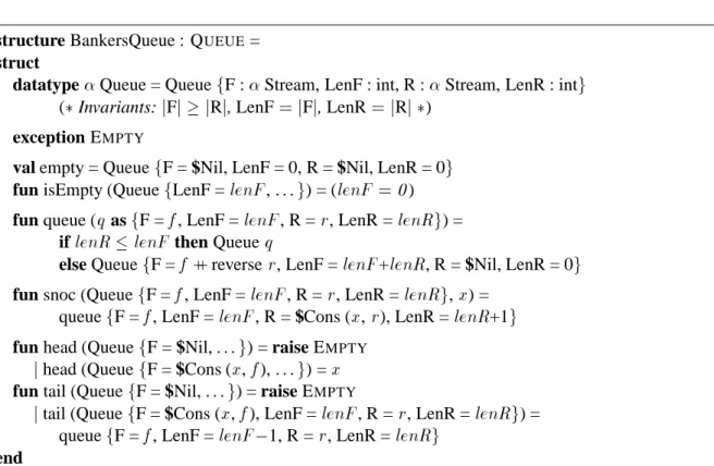
, R = $Nil, LenR = 0g

The complete code for this implementation appears in Figure 3.3.

structure BankersQueue : QUEUE=

struct

datatypeQueue = QueuefF :Stream, LenF : int, R :Stream, LenR : intg (Invariants:jFjjRj, LenF=jFj, LenR=jRj)

exception EMPTY

val empty = QueuefF = $Nil, LenF = 0, R = $Nil, LenR = 0g

fun isEmpty (QueuefLenF =

lenF

, . . .g) = (

lenF

=

0

)

fun queue (

q

asfF =

f

, LenF =

lenF

, R =

r

, LenR =

lenR

g) =

if

lenR

lenF

then Queue

q

else QueuefF =

f

++ reverse

r

, LenF =

lenF

+

lenR

, R = $Nil, LenR = 0g

fun snoc (QueuefF =

f

, LenF =

lenF

, R =

r

, LenR =

lenR

g,

x

) = queuefF =

f

, LenF =

lenF

, R = $Cons (

x

,

r

), LenR =

lenR

+1g

fun head (QueuefF = $Nil, . . .g) = raise EMPTY jhead (QueuefF = $Cons (

x

,

f

), . . .g) =

x

fun tail (QueuefF = $Nil, . . .g) = raise EMPTY

jtail (QueuefF = $Cons (

x

,

f

), LenF =

lenF

, R =

r

, LenR =

lenR

g) = queuefF =

f

, LenF =

lenF

;1, R =

r

, LenR =

lenR

g

end

Figure 3.3: Amortized queues using the banker’s method.

To understand how this implementation deals efficiently with persistence, consider the fol-lowing scenario. Let

q

0 be some queue whose front and rear streams are both of length

m

, and

let

q

i

=

tail

q

i;1, for

0

< i

m + 1

. The queue is rotated during the first application of

tail

,

and the

reverse

suspension created by the rotation is forced during the last application of

tail

. This reversal takes

m

steps, and its cost is amortized over the sequence

q

1

:::q

m. (For now, we

are concerned only with the cost of the

reverse

— we ignore the cost of the ++.)

Now, choose some branch point

k

, and repeat the calculation from

q

k to

q

m+1. (Note that

q

k

is used persistently.) Do this

d

times. How often is the

reverse

executed? It depends on whether the branch point

k

is before or after the rotation. Suppose

k

is after the rotation. In fact, suppose

k = m

so that each of the repeated branches is a single

tail

. Each of these branches forces the

reverse

suspension, but they each force the same suspension, so the

reverse

is executed only once. Memoization is crucial here — without memoization the

reverse

would be re-executed each time, for a total cost of

m(d + 1)

steps, with only

m + 1 + d

operations over which to amortize this cost. For large

d

, this would result in an

O(m)

amortized cost per operation, but memoization gives us an amortized cost of only

O(1)

per operation.

point just before the rotation). Then the first

tail

of each branch repeats the rotation and creates a new

reverse

suspension. This new suspension is forced in the last

tail

of each branch, executing the

reverse

. Because these are different suspensions, memoization does not help at all. The total cost of all the reversals is

m

d

, but now we have

(m + 1)(d + 1)

operations

over which to amortize this cost, yielding an amortized cost of

O(1)

per operation. The key is that we duplicate work only when we also duplicate the sequence of operations over which to amortize the cost of that work.

This informal argument shows that these queues require only

O(1)

amortized time per operation even when used persistently. We formalize this proof using the banker’s method.

By inspection, the unshared cost of every queue operation is

O(1)

. Therefore, to show that the amortized cost of every queue operation is

O(1)

, we must prove that discharging

O(1)

debits per operation suffices to pay off every suspension before it is forced. (In fact, only

snoc

and

tail

must discharge any debits.)

Let

d(i)

be the number of debits on the

i

th node of the front stream and let

D(i) =

P

ij=0

d(j)

be the cumulative number of debits on all nodes up to and including the

i

th node.

We maintain the following debit invariant:

D(i)

min(2i;

j

F

j;j

R

j

)

The

2i

term guarantees that all debits on the first node of the front stream have been discharged (since

d(0) = D(0)

2

0 = 0

), so this node may be forced at will (for instance, by

head

or

tail

). Thej

F

j;j

R

jterm guarantees that all debits in the entire queue have been discharged

whenever the streams are of equal length (i.e., just before the next rotation).

Theorem 3.1 The

snoc

and

tail

operations maintain the debit invariant by discharging one and two debits, respectively.

Proof: Every

snoc

operation that does not cause a rotation simply adds a new element to the rear stream, increasingj

R

j by one and decreasingj

F

j;j

R

j by one. This will cause the

invariant to be violated at any node for which

D(i)

was previously equal toj

F

j;j

R

j. We

can restore the invariant by discharging the first debit in the queue, which decreases every subsequent cumulative debit total by one. Similarly, every

tail

that does not cause a rotation simply removes an element from the front stream. This decreases j

F

j by one (and hence j

F

j;j

R

jby one), but, more importantly, it decreases the index

i

of every remaining node by

one, which in turn decreases

2i

by two. Discharging the first two debits in the queue restores the invariant. Finally, consider a

snoc

or

tail

that causes a rotation. Just before the rotation, we are guaranteed that all debits in the queue have been discharged, so, after the rotation, the only debits are those generated by the rotation itself. If j

F

j

=

m

andj

R

j

=

m + 1

at the time of