Two models for longitudinal item response data

TWO MODELS FOR LONGITUDINAL ITEM RESPONSE DATA

Cheryl D. Hill

A dissertation submitted to the faculty of the University of North Carolina at Chapel Hill in partial fulfillment of the requirements for the degree of Doctor of Philosophy in the

Department of Psychology (Quantitative).

Chapel Hill 2006

Approved by

Advisor: David Thissen, Ph.D. Reader: Patrick J. Curran, Ph.D. Reader: Andrea M. Hussong, Ph.D. Reader: Robert C. MacCallum, Ph.D.

ii ABSTRACT

Cheryl D. Hill: Two Models for Longitudinal Item Response Data (Under the direction of Dr. David Thissen)

Questionnaires are sometimes administered to the same sample of examinees on more than one occasion. Even when longitudinal data are available, researchers employing item

response theory (IRT) often use data only from the first administration for item calibration because there is likely a lack of conditional independence between responses to the same item from the same individual. However, in many longitudinal study designs, the sample size at one occasion is too small for reliable item calibration. Thus, a longitudinal IRT model for use with repeated measures study designs is desirable.

ACKNOWLEDGEMENTS

First, I would like to thank my advisor, Dr. David Thissen, for mentoring me during my graduate career. He always had an answer to my endless questions, and his insight into my research was invaluable. I appreciate his willingness to provide support, be it in the form of a research assistantship, travel funding, or introductions to others in our field. I am so fortunate to have had the opportunity to work with one of the great minds in psychometrics.

Thank you to my committee members: Dr. Patrick Curran, Dr. Andrea Hussong, Dr. Robert MacCallum, and Dr. Abigail Panter. Each of them has a very demanding

schedule, and I appreciate their taking the time to serve on my committee. They each brought a unique perspective to our discussions, and it was valuable having this diverse group to help shape my work.

iv

TABLE OF CONTENTS

Page

LIST OF TABLES... vi

LIST OF FIGURES... vii

CHAPTER 1 INTRODUCTION...1

1.1 Motivation for This Research ...1

1.2 Literature Review...1

1.3 The Unique Contribution of This Research ...5

1.4 Specific Aims of This Research...5

1.4.1 Aim 1...6

1.4.2 Aim 2...6

2 PROPOSED MODELS...7

2.1 A Local Dependence Approach to Longitudinal IRT...7

2.2 A Description of the Model as Latent Class Analysis ...13

2.3 An Alternative Model: A Bi-factor Analysis Approach to Longitudinal IRT ...14

3 ESTIMATION METHODS...17

3.1 Latent Class Analysis Estimation ...18

3.1.1 The E-step...18

3.2 Bi-factor Analysis Estimation...22

3.2.1 The E-step...22

3.2.2 The M-step...24

3.3 Bi-factor Analysis in Limited-Information Item Factor Analysis ...26

4 METHODS FOR EVALUATING THESE APPROACHES...28

4.1 Parameter Recovery with Simulated Data ...28

4.1.1 Simulation Parameters and Methods...28

4.1.2 2PL Method...31

4.1.3 CCFA Method...31

4.2 Model Evaluation with Empirical Data ...32

5 RESULTS...34

5.1 Simulated Data...34

5.1.1 Latent Class Analysis...34

5.1.2 Bi-factor Analysis...38

5.1.3 Comparison Between Latent Class Analysis and Bi-factor Analysis...42

5.2 Empirical Data ...46

5.2.1 Latent Class Analysis...46

5.2.2 Bi-factor Analysis...48

6 DISCUSSION...52

6.1 Evaluation of the Proposed Approaches ...52

vi

LIST OF TABLES

Table Page

1. Parameter recovery of data generated with the LCA model (N= 5000,I= 4)...59

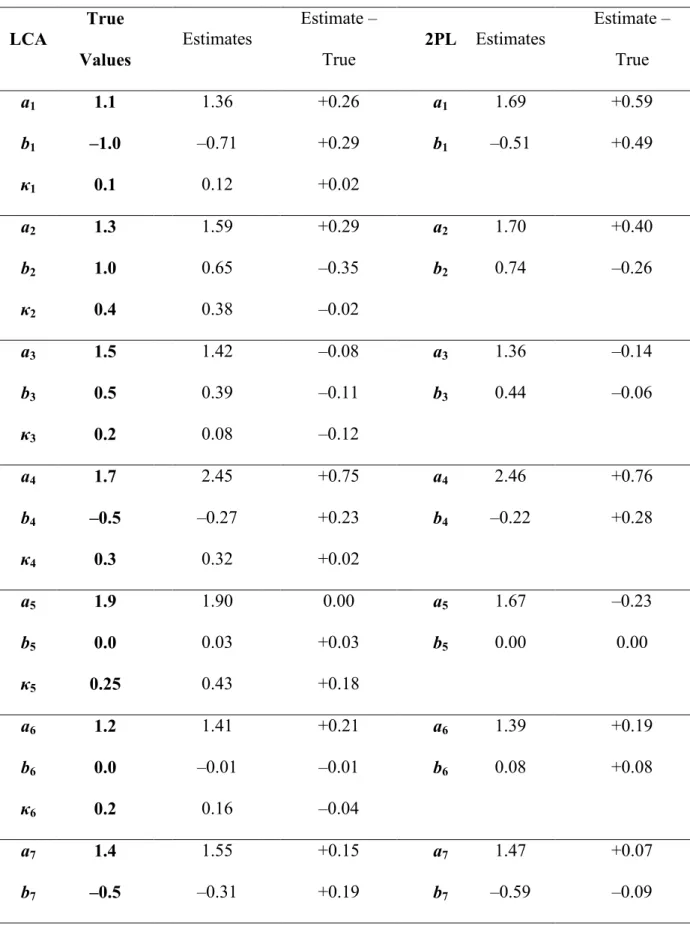
2. Parameter recovery of data generated with the LCA model (N= 100,I= 5)...60

3. Parameter recovery of data generated with the LCA model (N= 250,I= 5)...61

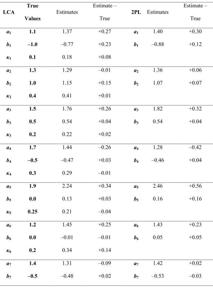
4. Parameter recovery of data generated with the LCA model (N= 500,I= 5)...62

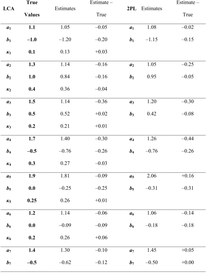
5. Parameter recovery of data generated with the LCA model (N= 100,I= 10)...63

6. Parameter recovery of data generated with the LCA model (N= 250,I= 10)...65

7. Parameter recovery of data generated with the LCA model (N= 500,I= 10)...67

8. Parameter recovery of data generated with the bi-factor model (N= 5000, I= 4)...69

9. Parameter recovery of data generated with the bi-factor model (N= 100,I= 5)...70

10. Parameter recovery of data generated with the bi-factor model (N= 250, I= 5)...71

11. Parameter recovery of data generated with the bi-factor model (N= 500, I= 5)...72

12. Parameter recovery of data generated with the bi-factor model (N= 100, I= 10)...73

13. Parameter recovery of data generated with the bi-factor model (N= 250, I= 10)...75

14. Parameter recovery of data generated with the bi-factor model (N= 500, I= 10)...78 15. Parameter estimates for the LCA model and the 2PL model

for items from a psychological distress scale in the Context Study (N= 3788, I= 4) 79 16. Parameter estimates for the bi-factor model and the CCFA model

LIST OF FIGURES

Figure Page 1. Longitudinal IRT model using a bi-factor analysis approach

(two items administered twice) ...81 2. Psychological distress items from the Understanding Adolescent

CHAPTER 1 INTRODUCTION

1.1 Motivation for This Research

Questionnaires are sometimes administered to the same sample of examinees on more than one occasion. This is often the case in psychological studies or clinical trials in which the effect of a treatment is modeled longitudinally. Traditionally, even when longitudinal data are available, researchers using item response theory (IRT) to develop or score a measure use the data from the first test administration for item calibration. This inefficient use of the data is due to the likely lack of conditional independence between responses by the same

individual, and the fact that implementations of IRT in software require conditional independence.

In many longitudinal study designs, the sample size is too small for reliable item

calibration using data from one occasion. Thus, it is desirable that a longitudinal IRT model be developed for use with repeated measures study designs. Using data from more than one occasion may provide additional information, effectively transforming a sample that is too small into one that is adequate for item calibration.

1.2 Literature Review

the validity of psychological measures. This technique uses different methods to measure different traits and hypothesizes the strength of association between the methods and traits. An example is a measure with multiple subscales measuring multiple outcomes, on which it is expected that the subscale intended to measure a particular outcome is more associated with that outcome than it is with other outcomes, and this outcome should be measured better by its corresponding subscale than by any other subscale. Another example might involve three people responding to a measure for themselves and for each other, in which case the MTMM approach would hypothesize that a person’s self-report responses would be more related to their trait than would be a friend’s responses about that person, and an

acquaintance’s responses regarding that person would be even less related to that person’s trait.

Kenny and Kashy (1992) suggested that MTMM methods could be evaluated using CFA, where the size of the factor loadings should vary in a predictable pattern. The model they propose that would apply to longitudinal response data is the correlated uniqueness model. In this model, there are multiple traits (i.e., trait factors), but the methods are represented with correlated unique factors across similar methods. For longitudinal item responses, the trait factors would be the latent trait of the measure over time. The unique factors for an item would be correlated over time, but disturbances for the other items would not correlate with that for the first over time. CFA parameter estimates can be converted into IRT parameters, so the results of an MTMM CFA approach to longitudinal data could be translated into item parameters and used in place of an IRT model.

3

analysis (CCFA) techniques exist and have improved considerably over the past two decades, but these techniques work best with large samples and simple models. Although this

approach is reasonable, it would not be ideal for many longitudinal study designs involving small sample sizes.

Hierarchical linear modeling (HLM) has also been applied in some form to longitudinal item response data. HLM is appropriate for data in which responses are nested within a higher level, for example, children nested within schools. Researchers have proposed combining IRT models with HLM techniques so that the standard errors for the individual latent traits from the IRT model can be used as information available in the higher order model. Often these higher levels involve the variables of interest to researchers, and

accounting for measurement error from the first level of the model can improve the accuracy of estimation in higher levels of the model. For the type of data considered here, individuals’ responses are nested within time.

Some researchers have used longitudinal Rasch modeling with HLM techniques using penalized quasi-likelihood estimation (e.g., Pastor & Beretvas, 2006; Raudenbush &

Sampson, 1999). In such models, the log odds is calculated for one fewer than the number of response categories for each item. Log odds models involve only a location parameter for each item, and assume a slope (or discrimination) parameter that is constant across items, so such models may not suit the needs of researchers who have longitudinal data from scales with varying levels of discrimination among the items.

extended to polytomous responses. These researchers were able to include this more

complicated IRT model in the HLM framework by replacing maximum likelihood estimation with Markov Chain Monte Carlo (MCMC) estimation. MCMC is a powerful estimation technique that can work for problems previously unsolvable with maximum likelihood estimation, but many applied researchers are not experienced with this complicated approach and may hesitate to use it.

Other researchers have applied traditional IRT techniques to repeated measures data by making relatively restrictive assumptions about the data. Ferrando, Lorenzo, and Molina (2001) considered the application of IRT to repeated measures, specifically to assess the stability of items over time. However, in the development of their model, they reason that the assumption of local independence is not violated because the latent trait is believed to be stable and the time between test administrations long enough for responses to be assumed independent of each other. Further, their model was designed to assess item stability over time when the items have already been calibrated. As a result, this model, while applicable to longitudinal data under certain conditions, is not relevant to researchers who hope to borrow information gained by multiple administrations for the purposes of item calibration.

5

the likelihood of a response pattern across time points is the product of the probability of the response to each item at each time; thus, independence between the items across the time points is assumed conditional on the entire vector of latent variable values across all times. This model is not an ideal approach because it ignores the possibility that local dependence (LD) appears between responses to the same item at different times. The dependence between the same items at different times may reflect an additional latent trait that is not accounted for in the one-trait-per-time design.

1.3 The Unique Contribution of This Research

The current literature on longitudinal item response data modeling covers some aspects of the problem of building an IRT model for repeated measures data; however, no complete solution has been offered. The existing models require the researcher to make assumptions (e.g., the item parameters are known or the latent trait is stable) that are unlikely to be true for many research designs. Alternative approaches are available, but the associated

estimation procedures may not be appropriate for small longitudinal datasets. Areas such as personality measurement, educational testing, and clinical trials can benefit from a

longitudinal IRT model that calibrates items while modeling change over time without requiring restrictive assumptions.

1.4 Specific Aims of This Research

parameters that describe the distribution of the latent trait at the second administration relative to the standardized distribution at time 1, and the correlation between the latent traits at two time points. The addition of these model components allows item parameters to be calibrated using available data from two occasions rather than limiting calibration to data from one time point.

1.4.1 Aim 1

The first set of research goals is to develop two approaches to longitudinal IRT, and to implement estimation algorithms for them. These models will be based on latent class analysis (LCA) and full-information bi-factor analysis, respectively. Maximum marginal likelihood parameter estimation will use the EM algorithm (Bock & Aitkin, 1981). The R statistical system (Ihaka & Gentleman, 1996) and C++ will be used to implement these estimation methods.

1.4.2 Aim 2

CHAPTER 2 PROPOSED MODELS

2.1 A Local Dependence Approach to Longitudinal IRT

Consider the probability of a particular response pattern for a set of items administered twice (without accounting for LD between administrations) as

= = = 2 1 2 1 2 1 1 ) ( ) | ( ) | ( t I i t

it ' '

u T

'

u

P , (1)

where uis a vector of responses, is a vector of latent trait values at time 1 and time 2, tis administration occasion, and iis item number within an administration (Iitems per

administration). For the 2PL model, useful for binary items that are not affected by guessing, the probability of endorsing an item is

)) ( exp( 1 1 ) | 1 ( i t i t it b ' a ' u T + =

= , (2)

where aiis the slope, or the strength of relationship between the response and the latent trait, and biis the threshold, or the location on 'twhere the examinee has a 50% probability of endorsing the item. Alternatively, the probability of not endorsing an item is

(

)

t

it ' T u '

u

T( =0| )=1 =1| . (3)

In (1), (')is the bivariate normal density, where

+ = 2 2 2 2 2 2 1 2 2 1 1 2 1 2 1 1 2 2 2 1 ) ( ) )( ( 2 ) ( ) 1 ( 2 1 exp -1 2H 1 ) ( µ µ µ

µ ' ' '

Here, µtis the mean of t, tis the standard deviation of t, and is the correlation between

'1and '2.

The model in (1) does not account for the LD among responses to the same item across time. To account for such likely LD, some sort of LD parameter must be added for each item pair. In developing an LD index for use in IRT, Chen and Thissen (1997) introduce HLD, the probability that the response to the second item is identical to the response to the first item without consideration of the latent trait. Alternatively, 1– HLD is the probability that the response to the second item is based solely upon the process implied by the IRT model without consideration of the response to the first item. When HLD is 1, the second item provides no information about the latent trait that is not available through the response to the first item. When HLD is 0, the two items each provide unique information about the latent trait. When HLD is somewhere between 0 and 1, the second item provides some new

information, but some of the information has already been captured through the response to the first item.

The same HLD parameterization may be used to represent the LD between two

administrations of the same item. In this context, each item will have an LD parameter, called

9

Consider a simple 2-item test that is administered twice. For dichotomous items in which 1 represents a correct or endorsed response and 0 represents an incorrect or non-endorsed response, uis a vector that refers the responses to item 1 at time 1, item 2 at time 1, item 1 at time 2, and item 2 at time 2. There are 16, or _{2 , possible response patterns:} 2I

• Neither item is repeated (u= 0011, 0110, 1001, or 1100);

• Item 1 is repeated but item 2 is not (u= 0001, 0100, 1011, or 1110);

• Item 2 is repeated but item 1 is not (u= 0010, 0111, 1000, or 1101); and

• Both items are repeated (u= 0000, 0101, 1010, or 1111).

When neither item is repeated, the examinee must have used the full IRT model when responding to each item at each time point (i.e., the LD model is not considered because neither item response was repeated).1Thus, the probability of each item response must be weighed by the probability of using the IRT model for both item 1 and item 2. This probability is written as

(

) (

)(

)

P ₁₁, ₂₁, ₁₂, ₂₂ = 1 ₁ 1 ₂ . (5)

In equation (5), the first subscript on urefers to the item number, the second subscript refers to the time, +iis the probability that item iwas repeated because of LD and not by chance, given the IRT model, and

=

2 1

2 1 2

22 2

12 1

21 1

11| ) ( | ) ( | ) ( | ) ( )

(u ' T u ' T u ' T u ' ' T

P_uuuu . (6)

The calculation of this probability involves all four item responses because they are (conditionally) independent of one another.

1_{In this model, only positive LD is included, where the response at time 2 is identical to response at time 1}

When item 1 is repeated but item 2 is not repeated, the examinee must have used the full IRT model when responding to item 2 at each time point, but either the IRT model or the LD model may have been used when responding to item 1 at time 2. In other words, the response to item 1 may have been repeated because '2led to the response, or because the response at time 1 was duplicated as the response at time 2. The probability equation for this response pattern must incorporate both the probability of using the IRT model for both item 1 and item 2 (first part of the sum), as well as the probability that the IRT model was used for item 2 and the LD model was used for item 1 (second part of the sum). This equation is

(

) (

)(

)

(

)

P ₁₁, ₂₁, ₁₂, ₂₂ = 1 ₁ 1 ₂ + ₁ 1 ₂ , (7)

where

=

2 1

2 1 2

22 1

21 1

11| ) ( | ) 1 ( | ) ( )

(u ' T u ' T u ' ' T

P_uuxu . (8)

Here, x represents the fact that the response to item 1 at time 2 does not factor in to the probability calculation. Thus, when a portion of the model represents the possibility that an item was repeated due to LD (e.g., P_uuxu), the probability of the response to that item at time 1 is included in the model but the probability of the response to that item at time 2 becomes 1 (i.e., the response at time 2 provides no information about '2).

A similar model is seen when the response to item 1 is not repeated but the response to item 2 is repeated, as in

(

) (

)(

)

(

)

P ₁₁, ₂₁, ₁₂, ₂₂ = 1 ₁ 1 ₂ + 1 _{1 2} (9)

11

while the response to item 2 at time 2 was based on the LD model (second part of the sum). Again, this second probability portion excludes the probability of item 2 at time 2 because, if the response was based on the LD model, then it contributes no additional information about the latent trait, which is seen in

= 2 1 2 1 2 12 1 21 1

11 | ) ( | ) ( | ) 1 ( )

(u ' T u ' T u ' ' T

P_uuux . (10)

Finally, if both items were repeated at time 2, then the probability of the response pattern is

(

) (

)(

)

(

)

(

)

u x uu uuuu P P P P u u u u P 2 1 2 1 2 1 2 1 22 12 21 11 1 1 1 1 , , , + + + = , (11)

which is a weighted combination of the probability that the responses at time 2 were based on the IRT model (first part of the sum), the probability that the response to item 1 at time 2 was based on the LD model while the response to item 2 at time 2 was based on the IRT model (second part of the sum), the probability that the response to item 2 at time 2 was based on the LD model while the response to item 1 at time 2 was based on the IRT model (third part of the sum), and the probability that both responses at time 2 were based on the LD model (fourth part of the sum). Here, the fourth probability only includes the responses at time 1 in the model, as in

= 2 1 2 1 1 21 1

11 | ) ( | ) 1 1 ( )

(u ' T u ' '

T

P_uuxx . (12)

equation isP_uuuu, which indicates that the probability of a response pattern is derived solely from the IRT model.

When either of the +iparameters are 1, the response to that item at time 2 is fully dependent on the response at time 1. The response at time 2 cannot be different from the response at time 1, so the eight possible response patterns in which that item is not repeated are not observed. For the eight remaining response patterns, the terms that account for the possibility that the repeated item response is due to the IRT model drop out of the equation (because 1–+iis 0).

When both +iparameters are 1, both responses at time 2 are fully dependent on the

responses at time 1. The responses at time 2 cannot be different from the responses at time 1, so only the last four possible response patterns in which both items are repeated are observed. In this case, the response pattern probability equation is simplyP_uuxx, which is the IRT model that includes only the responses at time 1.

To extend this approach to scales with Iitems (more than two), the probability of a response pattern, which involves comparing the response pattern, u, to each pof the 2I possible combinations of repeat patterns, is

( )

{ }

{ }

(

)

(

)

_{( )}

=

=1 2 1 1 1 1 1 2 2 1 2

p I i C I i I i i I

i pi

p i p u T u T B I A I u

P , (13)

where

{ }

1 p u

A

I _p , (14)

13 and

{ }

! " #

=

otherwise 1

and in repeated is

if

0 i p u

C

I _pi . (16)

In this generalized equation, indicator function Acontrols which of the possible probability portions are included in the total probability sum for that response pattern, indicator function Bcontrols the LD weights for that probability portion, and indicator function Ccontrols the inclusion of the item response probabilities in the time 2 product.

2.2 A Description of the Model as Latent Class Analysis

An alternative description of the model is as LCA. In the two items twice example, there are four latent classes of persons:

• The class that responds at time 2 by using the IRT model for both items (u= 0011, 0110, 1001, or 1100);

• The class that responds at time 2 by repeating the response to item 1 because of LD and using the IRT model for item 2 (u= 0001, 0100, 1011, or 1110);

• The class that responds at time 2 by repeating the response to item 2 because of LD and using the IRT model for item 1 (u= 0010, 0111, 1000, or 1101); and

• The class that responds at time 2 by repeating the responses to both items because of LD (u= 0000, 0101, 1010, or 1111).

(

)(

)

(

)

(

)

which imply that %₁+%₃ = ₁ and %₂+%₃ = ₂. The LCA parameters, -p, can be estimated using traditional LCA methods, and the +iparameters can be obtained from the values of -p. A general translation from +ito -pis

{ }

=

p pi p

i I D % , (18)

where

{ }

1 i p

D

I _pi . (19)

2.3 An Alternative Model: A Bi-factor Analysis Approach to Longitudinal IRT While the LCA approach to longitudinal IRT contains all of the components necessary for accounting for the LD among repeated items, it has the potential to create estimation

problems. Each item has an additional parameter for LD, and three more parameters are included for the 'distribution, so the number of parameters increases by over 50% as

compared to a traditional 2PL model. More importantly, the E-step becomes computationally demanding because the probability that corresponds to each latent class must be calculated for each response pattern. Thus, the size of the problem grows exponentially when a test becomes long, and sparseness in the latent classes may make +estimation difficult.

15

dimension and has a non-zero loading on no more than one secondary dimension. This bi-factor structure allows for simplified likelihood equations by reducing the integrations to two dimensions. Gibbons and Hedeker (1992) recognize that the bi-factor solution is an

alternative model for tests with locally dependent items.

In the bi-factor analysis approach to longitudinal IRT, instead of one primary factor and a collection of secondary factors, the model includes two primary factors (one for each 't) and Isecondary factors (one for each item). This bi-factor analysis approach permits the item parameters to be estimated using data from both time points (by constraining the item parameters to be equal within items across primary factors). Additionally, the LD is

accounted for by the secondary factors that capture the relationship between the responses for each item pair at time 1 and time 2.

In this approach, the probability of response pattern uis

( )

(

)

_{( )}

1 3 1 ,

t F j I i E I j t it j ij u T u

P . (20)

Here, tis time, jis the secondary factor, Fis the total number of factors (F= 2 +I),

(

)

_[

₍

₎

_]

1 , (21)

{ }

1 j i

E

I _ij , (22)

and

( )

(

)

(

) (

)

+

= µ µ

% 1 3 ₂ 1 exp 2 1 , (23)

where µis a vector of means for 'and is the covariance matrix for '. In (21),

(

)

i a b a b

CHAPTER 3

ESTIMATION METHODS

The parameters of either of these models for longitudinal IRT can be estimated using direct maximum likelihood, which maximizes the function

( )

(

)

=

u r log P u

l u , (24)

where ruis the observed number of examinees with response pattern u. However, direct maximum likelihood is not a practical estimation method for most data problems because computing time becomes excessive as parameters are added to the model (i.e., as test length increases). An alternative approach uses Dempster, Laird, and Rubin’s (1977) EM algorithm, as refined by Bock and Aitkin (1981) for IRT, by Mooijaart and van der Heijden (1992) for LCA, and by Gibbons and Hedeker (1992) for item bi-factor analysis.

The EM algorithm consists of two iterative steps: the expectation step (E-step) and the maximization step (M-step). In the E-step, the current values for the model parameters are used to estimate the number of people expected to be at each quadrature point, q, along ', the proportion of these people expected to endorse each item, and, in the LCA approach, the proportion of people expected to be in a particular latent class. In the M-step, these estimates are used as if they were observed data to obtain updated parameters. These two steps

3.1 Latent Class Analysis Estimation 3.1.1 The E-step

For the IRT portion of the estimation procedure, the goal of the E-step is to estimate the number of people at each quadrature point who endorse each item given the current values of the model parameters. This information is stored in a series of R* tables. *

1

i

R contains the expected number of examinees at each quadrature point that would endorse item i, while *

0

i

R

contains the expected number of examinees at each quadrature point that would not endorse item i. For dichotomous items, there are two R* tables for each item.

One of the goals in creating a longitudinal IRT model is to be able to combine data from two time points to calibrate one set of item parameters. Thus, the expected number of examinees at quadrature point qwho respond correctly to item iis a combination of the examinees at quadrature point qat time 1 and the examinees at quadrature point qat time 2, as in

(

) (

)

{ }

(

) (

)

+ =

u p Q

q up q q q q

i i p Q

q up q q q q

i u u qi L u C I L u P r r 1 1 1 1 2 2 2 2 , , , , ~ 2 1 *

1 , (25)

where

(

) { }

{ }

(

)

(

)

i i q

I

i pi

p q

q p

u I A I B T u T u pi

L

1 2

1 1

1 1 2

2

1, (26)

and

(

)

[

]

(

)

=

p q q

Q

q Q

q up q q

u L

P 1 2

2 2

1 1

2

1, ,

~

19

Summation over quadrature points replaces integration over 'in (13). P~uis used to normalize

the sum so that when it is multiplied by ru, the resulting value represents a number of persons.

For the time 1 responses, the values at each quadrature point of time 1 are summed across the quadrature points of time 2 and are included in the *

1

i

R calculation when item iwas endorsed. For the time 2 responses, the values at each quadrature point of time 2 are summed across the quadrature points of time 1, but they are only included in the *

1

i

R calculation when that item at time 2 was endorsed and used in the calculation of the probability for a particular part of the model (as controlled by indicator function C).

Conversely, the * 0

i

R calculation includes the response probability for item iwhen it is not endorsed at time 1, as well as when it is not endorsed but is used in the probability

calculation at time 2, which is written as

(

)

(

) (

)

{ } (

)

(

) (

)

+ =

u p Q

q up q q q q

i i

p Q

q up q q q q

i u u qi L u C I L u P r r 1 1 1 1 2 2 2 2 , , 1 , , 1 ~ 2 1 * 0 (28)

For the LCA portion of the estimation procedure, the goal of the E-step is to calculate the expected number of people with each response pattern in each latent class. This is calculated by

(

) (

)

2 2

1 1

2

1, ,

~ * q q Q q Q

q up q q

u u p u L P r

n = , (29)

where the latent class parameters are in the form of -prather than

{ }

= I

i pi

B I

1

and are

(

)

{ }

(

)

(

)

1 1 2

2

1, % (30)

For the distributional parameters of the population, the goal of the E-step is to create a matrix with the expected number of examinees at each quadrature point on 2-dimensional '. This is calculated as the sum of each of the latent class probabilities times the observed number of examinees with that response pattern summed across response patterns, which is written as

(

) (

)

[

]

=

u u p up q q q q

u q q L P r N 2 1 2 1 2

1 ~ , ,

* _{. (31)}

3.1.2 The M-step

In the M-step, the item parameters, the population parameters, and latent class parameters are calculated using the estimated data created in the E-step. The calculation of the item parameters takes the same form as it does for traditional unidimensional 2PL EM estimation. The log of the M-step likelihood function is maximized to obtain estimates for the item parameters, which is written as

( )

(

)

i r T r T

l log * log1

0 *

1 , (32)

21

(

)

(

)

i d ' a T + + = exp 1 1 , (33)

where diis –aibi. Using this slope-intercept form, the first derivative for the slope parameter is

(

)

(

)

l * *

1 , (34)

and the first derivative for the intercept parameter is

(

)

l * *

1 , (35)

where * 0 * 1 * qi qi

qi r r

N = + . (36)

The second derivative for the slope parameter is

(

)

[

]

the second derivative for the intercept parameter is

(

)

[

]

and second cross derivative for the slope parameter and intercept parameter is

(

)

[

]

The M-step calculation of the latent class parameter uses an approach suggested by Mooijaart and van der Heijden (1992), which is

= u p u p N n* ˆ

where *

p u

n is from (29) and Nis the total number of examinees. The latent class parameter estimates, %ˆ ,are then transformed into local dependence parameters,_p ˆ_i, by (18), which are used in the subsequent E step.

The M-step calculation of the population parameters uses the expected number of examinees at each quadrature point, *

2 1q

q

N from (31). The mean for the population at time tis

= 1 1 2 2 2 1 1 1 2 2 2 1 * * Q q Q

q q q Q

q Q

q q q q

t

N

N t

µ , (41)

the standard deviation for the population at time tis

(

)

q qq Q

q Q

q qq q t

t

N

N t µ

, (42)

and the population covariance is

2 1 2 1 * * 1 1 2 2 2 1 2 1 1 2 2 1 2 1 µ µ = Q q Q

q q q q Q

q Q

q q q q

N N

(43)

as formulated by Bock (1985). The values for µ2,*2, and )are then used as estimates in the next E-step, while the values for µ1and *1are replaced with fixed values, usually 0 and 1, respectively, to identify the scale of the latent variables.

23

However, the resulting R* tables are 2-dimensional ('tx'j), where the time 1 and time 2 responses are collapsed into one primary factor, 't. Repeated responses do not affect the inclusion or exclusion of data entered into the R* tables in the bi-factor approach.

The expected number of examinees at quadrature point qtxqjwho respond correctly to item iis a combination of the examinees at quadrature point q1xqj(at time 1) and the examinees at quadrature point q2xqj(at time 2), which is written as

(

) (

)

(

) (

)

1 , (44)

where

(

)

(

)

= = =

2

1 3 1 ,

, , 2 1 t F j I i E I q q i q q q

u j T t j ij

L , (45)

and

(

)

[

]

(

)

j

j

j q q q

Q q Q q Q q q q q u u L

P~ , , , ,

2 1 2 2 1 1 2 1

=

A similar calculation is used for the expected number of examinees at quadrature point qt xqjwho respond incorrectly to item i, where probabilities are included for incorrect

responses, which is written as

(

)

(

) (

)

(

)

(

) (

)

Additionally in the E-step, information about the 'distribution is obtained for use in the M-step. The 3-dimensional array of probabilities is multiplied by the observed number of examinees with that response pattern and summed across the quadrature points of the secondary factor, 'j. The resulting 2-dimensional array is summed across response patterns, creating an array of expected counts at each quadrature point of '1,2, as in

(

) (

)

N 1, 2, _~ 1, 2,

2 1

* _{, (48)}

3.2.2 The M-step

The M-step in the bi-factor approach is similar to the M-step in the LCA approach. For the item parameters, maximum likelihood multiple logit analysis is employed with the R* tables from the E-step. Again, the log of the likelihood function is maximized to obtain estimates for the item parameters, which is written as

( )

(

)

q qqi i

Q

q Q

q qqi i

i r T r T

l log * log1

0 *

1 , (49)

25

(

)

(

)

l * *

1 , (50)

and the first derivative for the intercept parameter is

(

)

q qq i qq i

i

T N r

d

l * *

1 , (51)

where * 0 * 1 * i q q i q q i q

qt j rt j rt j

N = + . (52)

The second derivative for either of the slope parameters is

(

)

(

)

q qq qqi i i

fi T T N a l 1 * 2 2 2 , (53)

the second derivative for the intercept parameter is

(

)

(

)

the second cross derivative for both slope parameters is

(

)

(

)

q N T T

a a l 1 * 2 1 2 2

1 , (55)

and the second cross derivative for either of the slope parameters and the intercept parameter is

(

)

(

)

For the population parameters, the same equations that were used for obtaining µ2,*2, and

3.3 Bi-factor Analysis in Limited-Information Item Factor Analysis

Because the item bi-factor analysis model is a full-information approach to Holzinger and Swineford’s (1937) bi-factor method, it is sensible to consider this approach in a CCFA framework as mentioned in the introduction in the context of MTMM techniques. This model is depicted as a structural equation model in Figure 1 for the simple case of two items

administered twice. This model includes two factors for the two administrations, '1and '2, and the items load only on the factor that corresponds to the time at which they were

administered. Factor loadings for the same item at different time points are constrained to be equal so that each item has one loading on the outcome of interest. The first factor is

standardized with a mean of 0 and a variance of 1, while the second factor has a mean of 52 and a variance of 622. The two factors have a covariance of 621.

The LD between the same item at different time points is captured in an error covariance (or correlation when the measured variables are standardized) between the two items. This error covariance could also be described as the square of the factor loading if each item pair loaded on its own LD factor with the two factor loadings constrained to be equal. Both parameterizations highlight the fact that the LD describes variance that the item pairs have in common above and beyond what is explained by the primary construct of interest.

27

The covariance between the responses to the same item at time 1 and time 2, 9i, can be translated into a slope for the secondary factor, aij, by the equation

(

)

i ij

a

,

-,

+ =

2

1 7 . 1

. (58)

The threshold, 7i, can be translated into an intercept, di, by the equation

(

)

i i

d

,

-.

+ =

2

1 . (59)

In these equations, the value 1.7 converts the estimates from the normal metric to the logistic metric which is specified in (21) (McLeod, Swygert, & Thissen, 2001).

This CCFA model can be estimated using the latent variable software Mplus (Muthén & Muthén, 2003) using weighted least squares (WLS) estimation when the sample is large or using diagonally weighted least squares with a mean- (and variance-) adjusted chi-square test statistic (WLSM/V) when the sample is small (Oranje, 2003). The CCFA converted

parameters should be similar to the IRT parameters when samples are large, but some

CHAPTER 4

METHODS FOR EVALUATING THESE APPROACHES When a new model is introduced, it is important to ask two questions: (1) can the parameters be estimated, and (2) are the estimates interpretable? These questions were considered for each of the two proposed approaches to modeling longitudinal IRT data. The first question was answered by using simulated data to evaluate the parameter recovery of each model. By using simulated data in which the true parameter values are known, the estimates can be compared to the true values to determine how well the algorithms estimate the parameters. The second question was answered using empirical data. The content of the items can indicate how stable the responses and the latent trait should be over time, and parameter estimates can be examined to determine if the hypothesized properties are revealed in the magnitude and sign of the estimates.

4.1 Parameter Recovery with Simulated Data 4.1.1 Simulation Parameters and Methods

First, data were simulated in the R statistical system for a large number of simulees (N= 5000) and a small number of dichotomous items (I= 4) at two time points. These data were used to evaluate the estimation procedures to ensure that they had been implemented

29

alternative model as an attempt to identify a link between the two approaches by comparing the parameter estimates.

Once the estimation methods were verified, data were simulated with smaller numbers of simulees (N= 100, 250, or 500) and larger numbers of items (I= 5 or 10). These conditions were chosen because they are comparable to the characteristics of data collected in

longitudinal study designs. The parameter estimates were compared to the true values to evaluate if the model can capture the parameters under these realistic conditions. It is important to demonstrate that the longitudinal IRT approach can recover the true parameter values for the data problems for which it is intended (i.e., many items with limited

examinees).

Further, it is desirable that the proposed models outperform existing methods in terms of parameter recovery. The parameter estimates of the LCA model were compared to those of the unidimensional 2PL model using data from one time point, and the parameter estimates of the bi-factor model were compared to that of the limited-information CCFA model using data from both time points.

For the LCA approach, true theta values were drawn from a 2-dimensional normal

is greater than or equal to the calculated probability, then the response is scored as negative. A provisional response at time 2 is simulated in the same manner using a new random

number and a probability calculated with the person’s true '2value. Because the +parameters can be considered as probabilities of repeating the response from time 1 at time 2, another random number is drawn from a rectangular distribution between 0 and 1. If the random number is less than the +value for that item, then the provisional response at time 2 is replaced with the person’s response at time 1. If the random number is greater than the +

value, then the provisional response is retained as the response at time 2.

For the bi-factor analysis approach, true theta values were drawn from a 3-dimensional normal distribution with a mean of 0 and a variance of 1 at time 1 and for the specific factor, and a mean of 0.2 and a variance of 1 at time 2. The correlation between '1and '2was .5, while '1and '2did not covary with the specific factor. True avalues on the dimension of interest varied between 1 and 2, true avalues on the LD dimension varied between 0.5 and 1.5, and true bvalues varied between -1 and 1 (thresholds were translated into intercepts given the slope values).

31

Within the estimation software, conservative starting values were chosen for the

parameters. The starting values for the distributional parameters were 0 for the mean at time 2, 1 for the variance at time 2, and 0.75 for the correlation between the two time points. For the LCA approach, avalues started at 1, bvalues started at 0, and +values started at 0.1. For the bi-factor approach, a1values started at 1, a2values started at 0.5, and dvalues started at 0. Because little was known about the properties of the likelihood surface for these models, strict convergence criteria were chosen to provide the routine ample opportunity to “climb” to the maximum value. Ten-thousand cycles were allowed, with estimation ending if the maximum change in estimated values from one cycle to the next dropped below 1.0e–07.

4.1.2 2PL Method

Parameter estimates from the LCA model were compared to those obtained using the 2PL model in Multilog (Thissen, Chen, & Bock, 2003). Data from the first administration alone were used for parameter calibration. Distributional statistics were calculated in SAS 9.1 (SAS Institute, Inc., 2005) using the sum of the item responses within administration and

standardizing the sample statistics at time 2 using the statistics from time 1. 4.1.3 CCFA Method

Parameter estimates from the bi-factor model were compared to those obtained using a longitudinal CCFA model in Mplus 3.13 (Muthén & Muthén, 2003). Although WLS

with WLSM/V. Thus, even if WLSM/V estimation was used for data with which WLS would be suitable, no error should be induced in the parameter estimates.

The model depicted in Figure 1 was specified in Mplus by letting each item load on the latent factor particular to its administration time, while constraining the factor loadings to be consistent across time within item. Means and thresholds were included in the model by specifying a mean structure analysis, and thresholds were also constrained equal across time within item. Error correlations were introduced between each item pair. Theta

parameterization, which allows the residual variances to be estimated in the model, was used. Each analysis was conducted on an inter-item tetrachoric correlation matrix by indicating that the data were categorical. Standardized estimates for factor loadings, error correlations, and thresholds were used in comparing CCFA results to bi-factor method results because IRT assumes that the underlying response variable is standard normal. CCFA estimates were translated into the IRT metric, and standard errors were translated using the delta method.

4.2 Model Evaluation with Empirical Data

33

were measured on a 5-point Likert response scale ranging from “Strongly agree” to “Strongly disagree”, and the item text is presented in Figure 2.

Data from adolescents at the first fall administration and the second spring administration (waves 2 and 3 of data collection) were chosen for the present analyses. Only participants who had no missing data on these 10 items across the two time points were included, which resulted in a sample of 3,788. This sample was 53% female and 57% white, with an average age of 13.5 (sd = 0.97) for the fall administration and 14.0 (sd = 0.97) at the spring

administration.

Prior to using these data to assess the proposed models, the dimensionality of this 10-item scale was assessed through a 1-factor CCFA model in Mplus. Local item dependencies were examined using modification indices for the error correlations between the measured

variables. It was established that several of the items were locally dependent, and the model was trimmed until one set of unidimensional, locally independent items was identified. After this item reduction, items 1, 2, 7 and 9 remained, and all subsequent analyses were conducted using this set of 4 items.

CHAPTER 5 RESULTS

5.1 Simulated Data 5.1.1 Latent Class Analysis

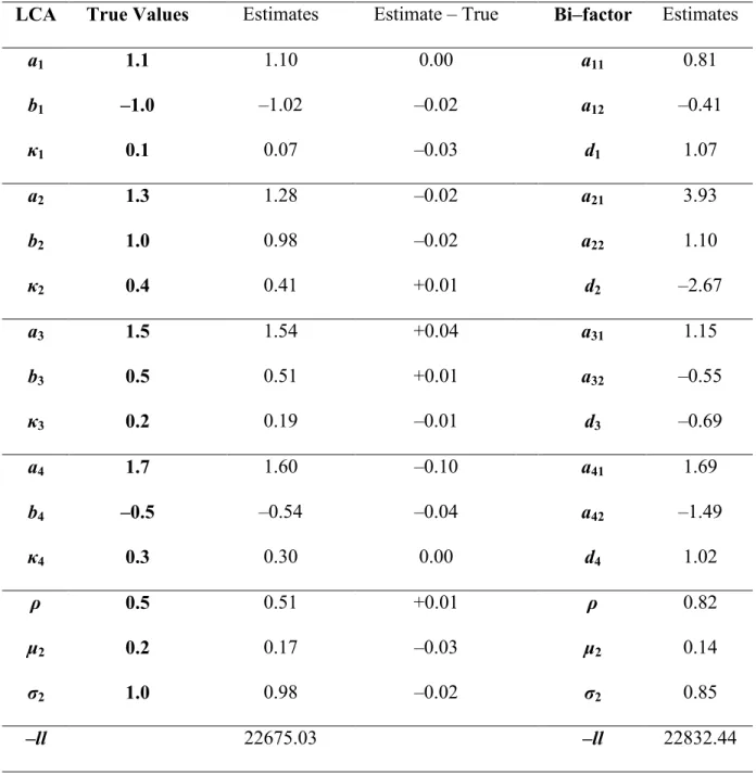
The programming of the LCA approach was evaluated using a simulated dataset of 5000 simulees and 4 items. The generating values, the parameter estimates, and the difference between the estimated and true values are presented in Table 1. The estimation procedure appears to work well for the LCA model, with differences between the estimated value and the true value being no more than 0.1 for the slope parameter, no more than 0.04 for the threshold parameter, and no more than 0.03 for the LD parameter. The difference between the estimated and true values was 0.01 for the correlation between '1and '2, 0.03 for the mean of '2, and 0.02 for the standard deviation of '2. These differences are very small and indicate good parameter recovery.

With the LCA algorithm implementation evaluated as correct, the analyses proceeded to evaluating parameter recovery under realistic data conditions. It is important to stress that parameter recovery was evaluated using one simulated dataset per data condition. Large parameter recovery simulation studies often use 1000 or more simulated datasets per

35

values. Aggregating over the whole set of data for one condition allows the true recovery to stand out while minimizing the effect of the odd samples. However, the present parameter recovery examination is intended to evaluate the potential of the proposed approaches, not to declare one method superior to another under specific conditions. If one or both approaches show value, then a larger simulation study to determine the conditions under which these methods are appropriate would be a logical next research step.

model, and for the threshold parameter, the differences ranged from –0.1 to +0.2 for the LCA model and 0 to +0.2 for the 2PL model. Again, both models captured the true parameter values suitably, and the more extreme difference in slope estimates was consistent between models, indicating randomness in sampling. The LD parameter estimates differed by –0.1 to +0.2 as compared to the true values. As in the 100 simulee dataset, both models captured the mean and standard deviation of the time 2 latent trait, but the 2PL model showed much more error in the correlation as compared to the LCA model (+0.4 versus +0.1).

In Table 4, the estimates for the sample of 500 simulees were similar to those for 250 simulees. Slope parameter errors ranged from –0.1 to +0.4 for the LCA model and from –0.2 to +0.6 for the 2PL model. Threshold parameter errors ranged from –0.2 to +0.2 for both models. The errors in the LD estimates ranged from –0.1 to +0.02. Again, both models provided good estimates for the mean and standard deviation of the latent trait at time 2, but the 2PL model produced a poorer estimate for the correlation between the latent traits (+0.3 versus –0.1). The consistency between the sample with 250 simulees and 500 simulees suggests that for 5 items, sample size greater than 250 has little impact on parameter recovery. Even with a small sample of 100 simulees, both models recovered the true

parameters acceptably, with the LCA model producing more accurate estimates than the 2PL model.

37

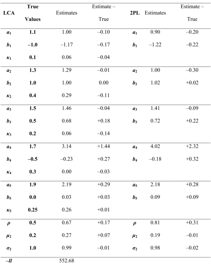
to +0.8 (MSE = 0.17) for the LCA model and from –0.2 to +0.8 (MSE = 0.14) for the 2PL model. Threshold parameter error ranged from –0.4 to +0.3 (MSE = 0.04) for the LCA model and from –0.3 to +0.5 (MSE = 0.05) for the 2PL model. Neither model recovered any

parameter perfectly, but the MSE was relatively small for the slope parameter and very small for the threshold parameter. Surprisingly, there was little difference between the two models in terms of parameter recovery of 2PL parameters. For the LD parameter, error ranged from –0.1 to +0.2 (MSE = 0.01), which is no worse than the 5-item samples. The two models showed little error in the '2mean (no error for the LCA model, –0.05 for the 2PL model), but they showed more error in the '2standard deviation (–0.21 for the LCA model, –0.17 for the 2PL model). As with the 5-item samples, the 2PL model poorly recovered the correlation parameter (error of +0.25) as compared to the LCA model (error of –0.05).

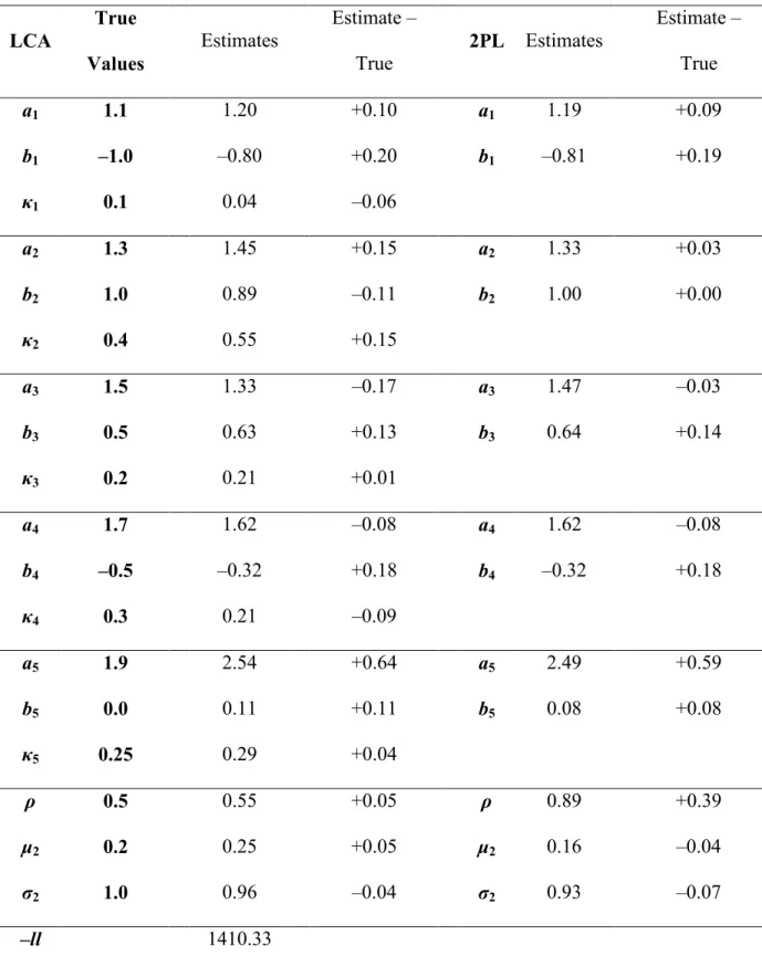
The results for the sample of 250 simulees in Table 6 showed better parameter recovery for both models. The slope parameter error for the LCA model ranged from –0.3 to +0.3 (MSE = 0.04) and ranged from –0.5 to +0.6 (MSE = 0.12) for the 2PL model. The threshold parameter error ranged from –0.1 to +0.2 (MSE = 0.01) for the LCA model and from –0.2 to +0.2 (MSE = 0.01) for the 2PL model. These ranges and MSE values show that both models recovered the 2PL parameters well with a sample of 250, with the LCA model providing more accuracy in the slope parameters than the 2PL model. The error in the LD parameters ranged from –0.04 to +0.1 (MSE = 0.003). This sample exhibited the same trend of good estimation for the mean and standard deviation of '2, with the 2PL model failing to recover the correlation as well as the LCA model (+0.3 versus +0.1).

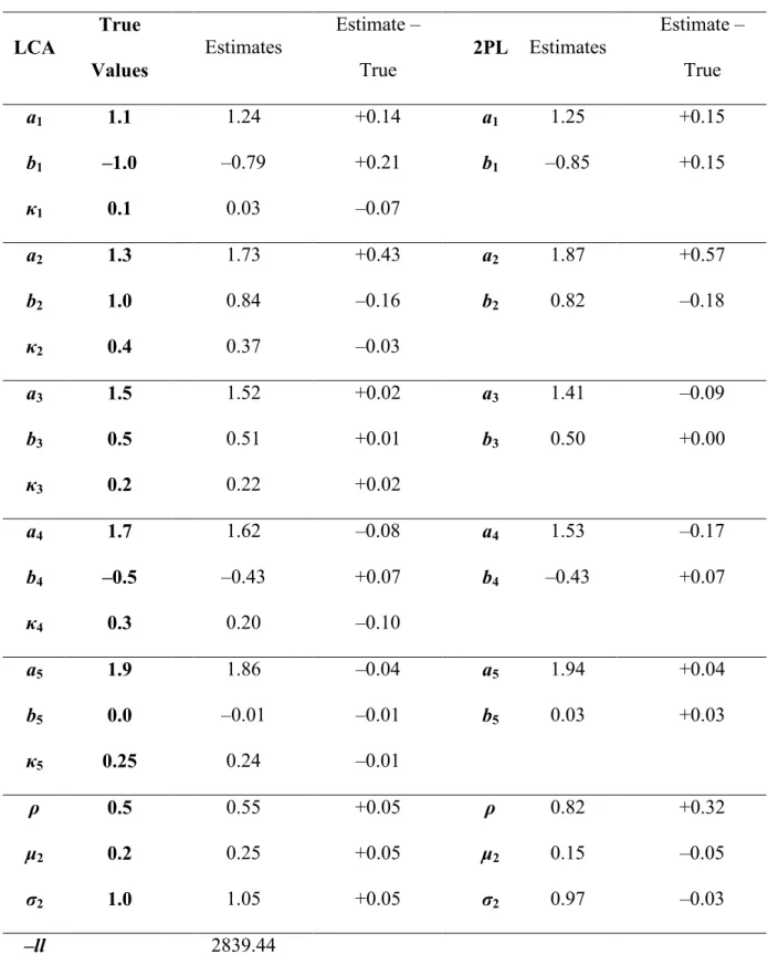
(MSE = 0.04) for the LCA model and from –0.4 to +0.3 (MSE = 0.07) for the 2PL model. The threshold parameter error ranged from –0.3 to +0.02 (MSE = 0.04) for the LCA model and from –0.3 to 0 (MSE = 0.03) for the 2PL model. With a sample of 500, the 2PL

parameters are recovered well using either model. The error for the LD parameters ranged from –0.04 to +0.06 (MSE = 0.001). The distributional parameters were recovered in the same manner as before, with the main difference being in the correlation for the 2PL model (+0.3) and the LCA model (–0.02).

Overall for the LCA model, parameter recovery is quite good. The approach shows promise for small samples and longer tests. Although there were no drastic differences in slope and threshold recovery between the LCA model and the 2PL model, the LCA model outperformed the 2PL model in distributional parameter recovery with its ability to include the distributional parameters as part of the full-information model. The LCA model also had success in recovering the LD parameters across all data conditions.

5.1.2 Bi-factor Analysis

39

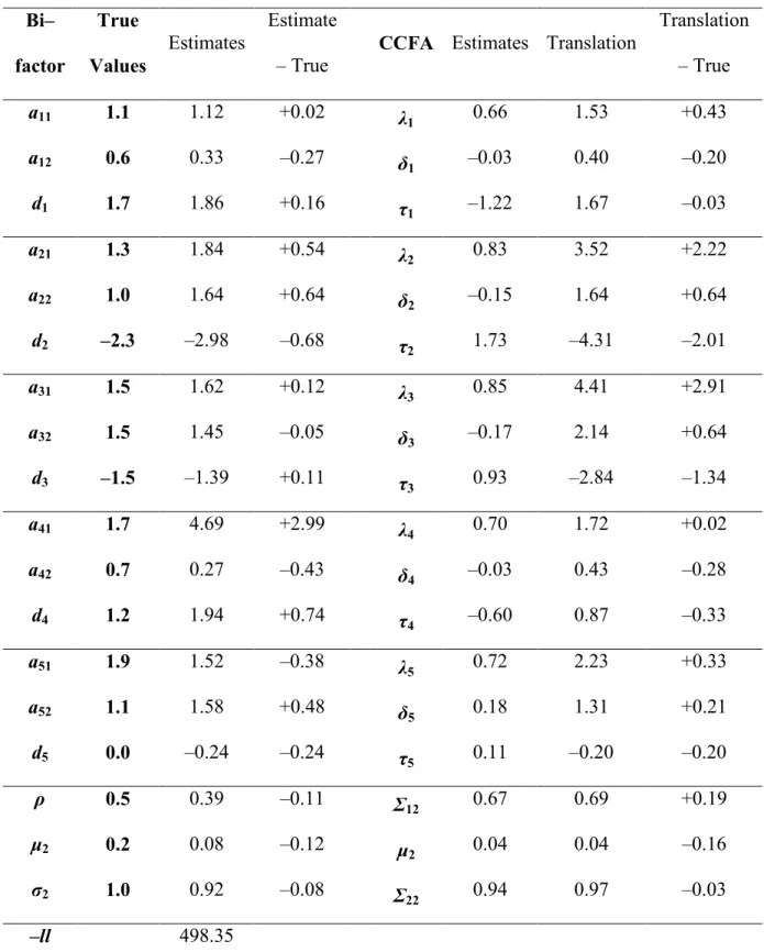
With the programming verified, analyses switched to parameter recovery evaluation using samples generated with the bi-factor model with the same characteristics as those generated using the LCA model. Responses to a 5-item test were simulated for samples of 100, 250, and 500. Results for the 100 simulee sample are presented in Table 9. Estimation errors in the slopes on the primary dimension ranged from –0.4 to +3.0 for the bi-factor model and from +0.02 to +2.9 for the CCFA model. The items for which the largest difference between the estimates and the true values were observed were not consistent between models, suggesting that the error is not a result of an odd sample. The errors for the LD slopes ranged from –0.4 to +0.6 for the bi-factor model and from –0.3 to +0.6 for the CCFA model. The difference between the estimated intercept values and their true values ranged from –0.7 to +0.7 for the bi-factor model and from –2.0 to –0.03 for the CCFA model. The CCFA estimation

algorithm did not capture the threshold parameters as well as the bi-factor model, while both models exhibited similar levels of error in their slope estimates. In comparing distributional parameters, the bi-factor model showed slightly less error in the '2mean and in the

correlation between '1and '2(–0.1 versus –0.2 for both parameters), while the bi-factor model showed slightly more error in the '2standard deviation (–0.1 versus –0.03).

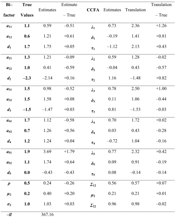
slope parameter recovery for the primary dimension was somewhat better for the CCFA model than the bi-factor model in this sample. The bi-factor model had larger estimation errors than the CCFA model for the '2mean (error of +0.2 versus +0.01 for CCFA) and the correlation between '1and '2(error of –0.3 versus +0.1 for CCFA). Error was similar for the

'2standard deviation for both models.

The results for the sample of 500 are presented in Table 11. Error of estimation in the slope parameters on the primary dimension ranged from +0.1 to +1.7 for the bi-factor model and from +0.3 to +0.8 for the CCFA model. Error in the slope parameters on the LD

dimension ranged from –1.3 to –0.1 for the bi-factor model and from –0.7 to –0.1 for the CCFA model. Error in the intercept parameters ranged from 0 to +0.1 for the bi-factor model and from –0.3 to +0.5 for the CCFA model. Although the error decreases for this sample with 500 simulees as compared to the samples with 100 and 250 simulees, the CCFA model did not show improvement in capturing the intercept parameters, while the bi-factor model (more so than the CCFA model) did not show improvement in slope parameter estimation. The distributional parameters continue to have relatively large errors for this sample with both methods. For both models error was –0.1 for the mean and standard deviation of '2and +0.1 for the correlation between '1and '2.

41

and +1.1 (MSE = 0.23) for the bi-factor model and between –1.0 and +2.0 (MSE = 0.72) for the CCFA model. As with the 5-item examples, neither model precisely captures the slope parameters with 100 simulees, but the MSE values show that the bi-factor model provided more accurate estimates. Error in the intercept parameters ranged from –0.8 to +0.9 (MSE = 0.25) for the bi-factor model and from –4.3 and +0.6 (MSE = 2.26) for the CCFA model. Again, the CCFA model produces poor intercept parameter estimates with a small sample. Estimates for the distributional parameters did not worsen for this longer test with the mean and standard deviation error being –0.1 for both models, while the correlation estimation error was –0.02 for the bi-factor model and +0.2 for the CCFA model.

Results for 250 simulees and 10 items are presented in Table 13. Parameter estimation improved considerably with this increase in sample size. Primary slope estimation error was between –0.6 and +0.3 (MSE = 0.09) for the bi-factor model and between –0.2 and +1.0 (MSE = 0.30) for the CCFA model. LD slope error ranged from –0.03 to +0.8 (MSE = 0.10) for the bi-factor model and from –1.0 and +1.4 (MSE = 0.54) for the CCFA model. Intercept error of estimation varied from 0 to +0.4 (MSE = 0.04) for the bi-factor model and from –0.1 to +1.2 (MSE = 0.18) for the CCFA model. These MSE values were acceptable for the bi-factor model, while they remained inflated for the CCFA model. The distributional parameter estimation error was similar between the models and accuracy did not improve using this sample. Mean error was –0.2 for both items, standard deviation error was –0.04 for the bi-factor model and +0.1 for the CCFA model, and correlation error was –0.1 for the bi-bi-factor model and +0.2 for the CCFA model.

primary slope was between –0.2 and +1.0 (MSE = 0.16) for the bi-factor model and between +0.1 and +0.6 (MSE = 0.22) for the CCFA model. Estimation error in the LD slope varied from –0.4 to –0.1 (MSE = 0.07) for the bi-factor model and from –1.2 to +0.4 (MSE = 0.40) for the CCFA model. Error in the intercept ranged from –0.2 to +0.4 (MSE = 0.03) for the bi-factor model and from –0.3 to +0.2 (MSE = 0.04) for the CCFA model. The bi-bi-factor model recovered the parameters better than the CCFA model, though there was little difference in the intercept errors between the models. Results for the distributional parameters are consistent with what was seen in other examples. The mean, standard deviation, and

correlation errors were +0.01, –0.2, and +0.1, respectively, for the bi-factor model and were –0.01, –0.04, and +0.2, respectively, for the CCFA model.

Overall, the bi-factor model estimation algorithm did not capture the true parameters as well as the LCA model. Both the bi-factor model and the CCFA model performed well in estimating distributional parameters, but both models were sensitive to sample size and test length in estimating slopes and intercepts. Although it is difficult to outline data conditions necessary for accurate estimation using these few examples, the bi-factor model showed improvement in parameter recovery for the test with 10 items and 250 simulees.

5.1.3 Comparison Between Latent Class Analysis and Bi-factor Analysis

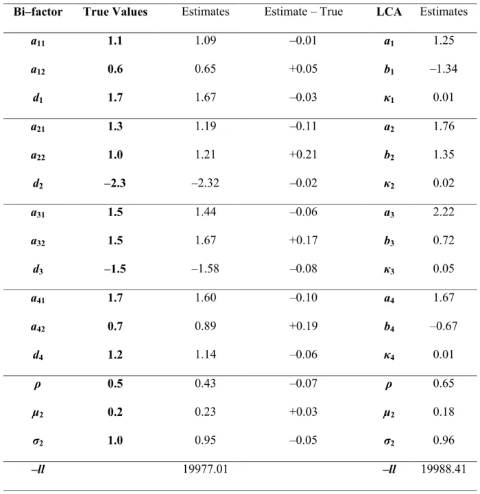
In addition to evaluating the parameter recovery of the LCA and bi-factor models, simulated data were used to investigate the relation between the two models. In Table 1 parameter estimates from the bi-factor model are presented for the example with 5000

43

threshold using the formula bi= –di/(ai1+ai2)) would correspond to the LCA threshold. The connection between the LD parameter in the LCA model and the LD slope in the bi-factor model was unknown; the first is a probability of repeating the response from time 1 at time 2 and the second is a correlation between the responses at time 1 and time 2. The slopes and thresholds appear to correspond as expected, but some are estimated more precisely than others in the bi-factor model. The differences between the estimated bi-factor primary slope and the true LCA slope are –0.3, +2.6, –0.4, and –0.01, respectively, for each of the four items. The bi-factor intercept estimates are –0.88, 0.53, 0.41, and –0.32, respectively, for each of the four items, in terms of threshold reparameterization. These values differ from the true LCA threshold values by +0.1, –0.5, –0.1, and +0.2. Thus, for these known parameters of the bi-factor model, the estimates do not correspond to the true values as closely as would be expected with a sample of 5000. It is possible that generating data according to the LCA model and fitting it with the bi-factor model induces error in the parameter estimates that does not appear when the same models are used for simulation and estimation. Additionally, the distributional parameters for the bi-factor model did not correspond exactly to the true values. The mean differed by –0.06, the standard deviation by –0.15, and the correlation by +0.32.

In terms of the connection between the LD parameters in the two models, the order of increasing LD slopes for the bi-factor model is similar to the order of increasing LD