Fingerprint resampling: A generic method for efficient resampling

Fingerprint resampling: A generic

method for efficient resampling

In resampling methods, such as bootstrapping or cross validation, a very similar computational problem (usually an optimization procedure) is solved over and over again for a set of very similar data sets. If it is computationally burdensome to solve this computational problem once, the whole resampling method can become unfeasible. However, because the computational problems and data sets are so similar, the speed of the resampling method may be increased by taking advantage of these similarities in method and data. As a generic solution, we propose to learn the relation between the resampled data sets and their corresponding optima. Using this learned knowledge, we are then able to predict the optima associated with new resampled data sets. First, these predicted optima are used as starting values for the optimization process. Once the predictions become accurate enough, the optimization process may even be omitted completely, thereby greatly decreasing the computational burden. The suggested method is validated using two simple problems (where the results can be verified analytically) and two real-life problems (i.e., the bootstrap of a mixed model and a generalized extreme value distribution). The proposed method led on average to a tenfold increase in speed of the resampling method.

Resampling methods refer to a variety of different procedures in which a Monte Carlo method is used to create a large number of resampled versions of the original data. Well known examples include boot-strapping1_{, permutation tests and various sorts of cross-validation. Commonly, resampling methods are}

used to assess the uncertainty of an estimator, to estimate tail area probabilities for hypothesis testing, to assess prediction errors or to do model selection2_.

Broadly speaking, all resampling methods follow the same general scheme. First, the original data set is resampled multiple times. Resampling can be done directly on the original data set or through a statistical model that is first fitted to the data. In a next step, a model is estimated for the resampled data. Finally, the results of the estimated models are combined to calculate, for example, the uncertainty of an estimator of interest (e.g., confidence intervals and predictive validity obtained using bootstrapping and cross-validation, respectively).

A major reason for the popularity of these resampling methods stems from their flexibility3–7_{. They}

allow a researcher to compute uncertainty assessments or hypothesis tests in situations where no ana-lytical solution is available or where some assumptions of the anaana-lytical method are not justified (e.g., deviations from normality).

Unfortunately, even in these times of abundant computer power, a main disadvantage of these res-ampling methods is the computational burden. This computational burden is specifically present when for every regenerated data set, an iterative method is needed to maximize a likelihood or to minimize a squared error. If such an optimization is costly, the resampling method may become practically unfeasible.

As an illustration of the problem, one may think of the calculation of a bootstrap based confidence interval (CI) for a variance component in a linear mixed model8_{. Linear mixed models are commonly}

used in the life sciences9–13_{. More specifically, we consider a data set and model described in Samuh et al}14_.

A sample of 129 depressed individuals is measured 71 times on average (in total there are about 9115 time points) regarding their momentary sadness. The design is unbalanced because not all individuals have the same number of measurements. A longitudinal linear mixed model (see Verbeke and Molenberghs8₎

1_{University of Leuven, Oude Markt 13, 3000 Leuven, Belgium.} 2_{Leiden University, Rapenburg 70, 2311 EZ Leiden,} Netherlands. Correspondence and requests for materials should be addressed to M.M. (email: merijn.mestdagh@ ppw.kuleuven.be)

received: 07 May 2015 accepted: 22 October 2015 Published: 24 November 2015

with the previous emotional state as a predictor is fitted to the data. Both intercept and slope are assumed to vary randomly across patients.

Our prime interest for these data is in the variance components (i.e., the estimates of the between patient variances regarding intercept and slope). Current analytical procedures for computing such a variance component CI are not accurate enough and therefore a bootstrap based CI is pursued as an alternative15–17_{. If we aim at 2000 bootstrap replications, then repeatedly fitting the linear mixed model}

would take more than four hours using one core on an Intel Core i7-3770 with 3.4 GHz computer. Such computation times may prohibit the routine use of the bootstrap by applied researchers.

Together with the rise in popularity of resampling methods, there have been continued efforts to alle-viate the computational burden of these methods. For example, Efron and Bradley proposed to decrease the number of bootstraps in favorable cases18_{. They improved the post processing of the bootstrap}

esti-mates, increasing the accuracy for the same number of bootstrap estimates computed. However, most efforts are concentrated on decreasing the computational burden of the model fit on a single resampled data set by, for example, reducing the number of iterations in the optimization method9–21_{. Another way}

to speed up the resampling process is to split the estimating function into smaller, more simple parts. Bootstrapping these parts can lead to faster and more accurate bootstrapping22_{. More recent}

improve-ments focus on tailor-made solutions for specific problems23–25_{. Unfortunately, none of these methods}

are generic and easily convertible to other situations.

In this paper, we will propose a generic procedure to decrease the computational burden. As a result, resampling methods can be used for problems that are very time-consuming because an iterative opti-mization is needed. The key idea of our method is that for all resampled data, a similar task has to be performed because the same model has to be fitted to very similar data. Consequently, when this task is performed repeatedly, we may learn from the past and use this knowledge for future problems. This core idea is very simple and can be applied to any resampling technique.

More specifically, the optimization algorithm needs an initial (or starting) value for each resampled data set. By improving the quality of this initial value, the optimization problem can be significantly speeded up because the closer the initial value to the real optimum, the less iterations the algorithm needs to converge. The method we propose will use information from previous fits to considerably improve the starting points for subsequent problems. In addition, if the initial value is accurate enough, the optimization process may even be omitted.

Results

An optimal choice of the starting values. Two simple examples (involving the exponential distri-bution and a simple linear regression) will be used to motivate and introduce our method on how to choose the starting values of numerical optimization algorithms in a resampling context optimally. In both examples, there are two artificial aspects that make them simple examples. First, we will make use of the bootstrap in both situations, but the simple and well-understood properties of these models make the use of the bootstrap unnecessary. Second, our proposed method will only provide an advantage if the estimation process makes use of a numerical optimization algorithm. However, for both examples, closed-form estimators are available. Therefore, we will nevertheless make use of an iterative optimization algorithm and act as if the analytical solution is not known. An advantage of working with such simple models with available closed-form expressions is that some results can be checked analytically.

In a first example, we will bootstrap an exponential distribution. The loglikelihood of such an expo-nential distribution, with data set X= ( ,..., )x1 x_n is given by

θ θ

θ

( ) = − ( ) − ∑= . _{( )}

 ;X nlog in 1xi ₁

For a positive θ, the maximum of this equation is found by setting its first derivative to zero:

θ

θ θ θ

( )

= − + ∑= = _{( )}



d X

d

n x

;

0 ₂

i n

i

1 2

and solving for θ:

θˆ= ∑=x = . _{( )}

n x 3

i n

i

1

The resulting optimum is the sample average, x. The analytical solution will only be used to verify our findings and to provide a better insight in the workings of our method. Let us now simulate a data set, denoted as the original data X0, with θ= 2, θˆ0=x0= .2 1 and n= 100. For the bootstrapping process,

the data sets are non-parametrically resampled B= 200 times ( ,X X X1 2, _b,...,X200). The loglikelihoods of

the original data set and 200 resampled data sets are shown in Fig. 1a.

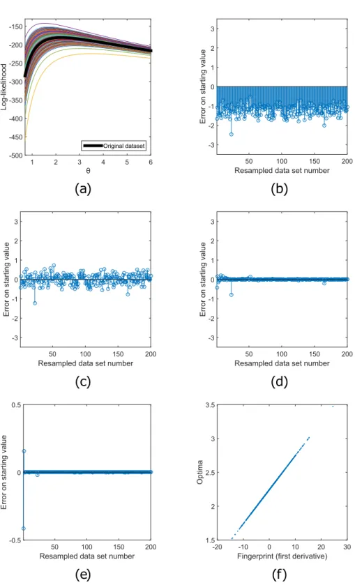
Figure 1. Choosing optimal starting values for an exponential model. In (a) the loglikelihood functions of the exponential distribution for the original data set and 200 resampled data sets are shown. The optima (θˆ) of all these loglikelihood functions need to be found using an iterative optimization proces. Each optimization needs a starting value θ. In (b–e), the horizontal axis shows the resampled data set number b and the vertical axis the initial errors on the starting values _E =θ −θ^

b b b. In (b), option 1 is used to choose

this starting value (θ=1). All initial errors are negative. (c) shows that this bias of the starting values can be avoided by using option 2. The original optimum, θˆ0 is more central compared to the other optima. In (d) it is shown that this error decreases further when the nearest neighbor variant of option 3 is used. In (e), where the interpolation variant of option 3 is used, the error almost vanishes. Using first order derivatives as fingerprint, the optima are easy to predict. In (f) it is shown that there is a linear relation between

value, θ_b. (In the remainder of the paper, we will denote starting values by a tilde.) The closer the starting value to the optimum, the faster the optimization algorithm will converge to the optimum. The difference between the starting value and the optimum for a bootstrap sample, θ_b−θˆ_b, will be called the initial error and denoted as E_b.

Let us now consider in turn three options we have when choosing these starting values for the B

bootstrap samples.

Option 1: A naive starting value. In an extreme situation, the researcher barely knows anything about the problem at hand and chooses a common naive starting value, for example, θ_b=1 (for all b). The initial error corresponding with this naive starting value, Eb=θb−θˆb= −1 θˆb, is shown in Fig.  1b for all

resampled data sets. In this case, the starting value is clearly an underestimation of the optimum, and the error is always negative.

Option 2: The original optimum θˆ₀ as a starting point. An easy improvement can be made at this point by taking the original optimum as a starting value:

θ θ

∀b: _b= .ˆ0 ( )4

The original optimum, θˆ₀, is the optimum that belongs to the fit of the original data set X0 and is

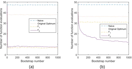
typically computed before the resampling process anyway. All the subsequent regenerated data sets, X_b, are related to this original data set. The original data set can be considered central. As a consequence, it is likely that also θˆ₀ is central to the optima of the resampled data sets, as is the case in Fig. 1a. This leads to a much less biased starting value (Fig. 1c) and a faster optimization process (Fig. 2a).

Option 3: Learn from the previously resampled data sets. The starting value can be improved upon fur-ther. The same function (Eq. 1), based on very similar data sets (all resampled from X0), needs to be

optimized over and over again. As a result, all the loglikelihoods look very similar, as shown in Fig. 1a. The core of our method lies in the fact that we try to learn from the past. When one needs to find the estimate θˆ_b for resampled data set X_b, the optima belonging to all previous data sets, θˆ₁ to θˆ_b−1, are already found. If b goes to infinity, the optimum of the same data set will already be computed. A better starting value cannot be wished for.

In the more realistic setting of a finite b, X_b will not be in the set of {X1,...,X_b−1}. There will however be some data sets that are more similar to X_b than others. One can search now for the most similar data set. Assume X_j is the most similar data set to Xb. The optimum θˆj of this similar data set will probably

be a good prediction of the optimum belonging to data set Xb. We can take this prediction as a starting

value, θ_b=θˆ_j. One can call this a nearest neighbor prediction:

(

)

θb=θˆj⇔ j< | ∀ <b k b d X X: ( ,j b) ≤ ( ,d X Xk b) , _{( )5}

with d(Xj, Xb) a distance between data sets Xj and Xb. If b gets larger, more and more resampled data

sets are fitted leading to a larger pool of previous data sets to choose from. The chances of finding a very similar data set become larger, leading to better starting values.

Although intuitive to grasp, measuring the distance between raw data sets is often not very easy. A better strategy is to first summarize the resampled data sets into properties (or statistics) that carry information about the optima. Such summary statistics will be called fingerprints. A fingerprint  is a statistic or function that takes a resampled data set as input. The idea is that these statistics provide direct information on the optimum that we look for. In general, we propose to use derivative-based finger-prints. In this exponential distribution example, the first derivative of the loglikelihood for the resampled data set evaluated in the original optimum will suffice. Formally, the fingerprint for the resampled data

b is defined as:

 θ_θ

θ _θ

= ( ) = − + ,

( ) θ θ

,

=



ˆ _ˆ

ˆ

d X

d

n nx

;

6

b b b

1

0 ₀2

0

with x_b being the sample average of resampled data set X_b. Here the first index of 1,b refers to the fact

that the first order derivative is used.

Once the derivative-based fingerprints ℱ are computed, we can just take the squared Euclidean dis-tance between them to create a disdis-tance measure between the resampled data sets:

 

( , ) = ( _, − _,)

d X X_{j b} 1_j 1_b 2. In Fig.  1d the initial errors Eb in the starting values computed using

Equations 5 and 6 are shown. It is shown that the errors become on average considerably smaller when the number of fitted bootstrap samples increases.

A disadvantage of the nearest neighbor approach is that when a new fingerprint 1,b becomes

avail-able, only the nearest neighbors to this new fingerprint determine the newly assigned starting point θ_b. However, we can improve on this practice by using a clever interpolation method. We want to model the relation between the already computed fingerprints 1_,j( = , …, − )j 1 b 1 and their corresponding optima

θˆj( = , …, − )j 1 b 1. This relation can then be used to make a prediction and to associate a good starting point θ_b to the new fingerprint 1,b.

Because we do not know much about the relation we want to model in general, we choose an inter-polation method that is capable of capturing nonlinear relations. Examples of such methods are least squares support vector machines (LS-SVM)26,27 _{or multivariate adaptive regression splines (MARS)}28_{. We}

will show only the results obtained by using LS-SVM, however similar results were obtained by using MARS.

The goal of the nonlinear interpolators is to learn the relation f:θ based on the couples (1 1,, )θˆ1

to (1, −b 1,θˆb−1). The estimated relation can be denoted as ˆf1: 1b− (where the index indicates that the first −

b 1 data sets are used). In a next step, the optimum of resampled data set X_b can be predicted:



θˆbpred=fˆ1: 1b₋ ( 1,b). ( )7

The predicted optimum will then serve as the improved starting point for the resampled data X_b:

θ_b=θˆ_bpred. ( )8

will not discuss the nearest neighbor variant anymore and directly consider this interpolation method as it gives much better results.

In fact, after two bootstrap samples, the predicted optimum actually coincides with the true optimum for the resampled data set. Hence, the interpolation method can, based on the fingerprint, almost exactly predict the optimum. This is not a surprise because in this exceptionally easy toy example, there exists an exact functional relation between the fingerprint and optimum. This can be seen when one combines Equation 6 and the analytical solution of the maximum likelihood estimation (Eq. 3):



θˆ = = θ , + .θ _{( )}

ˆ _ˆ

x

n 9

b b 0 b

2

1 0

Because of the linearity of this relation, only a set of two training points (Fig. 1e) is enough to create a model that delivers almost perfect starting values, instantly leading to fast optimizations (Fig. 2a). The relation between the fingerprints and the optima for all the resampled data sets is shown in Fig. 1f.

The options to choose a starting value, described in the previous paragraphs, are generic and can easily be used for other estimation problems. In a second example, they are applied to a linear regression without intercept and with known variance. In Figs 3 and 2b similar results are shown for options 1 and 2. However, for option 3, a one dimensional fingerprint, using only the first order derivative of the loglikelihood, is not sufficient anymore. The accuracy of the starting values improves if also the second order derivative is used, called the F2 variant. The starting values are now predicted using a two

dimen-sional fingerprint:

 

θˆpredb =ˆf1: 1_b− ( 1,b, 2,b). ( )10

As this new relation is nonlinear (Fig. 3f), it takes more bootstrap samples to be learned, which leads to a more gradual decrease in function evaluations, as shown in Fig. 2b.

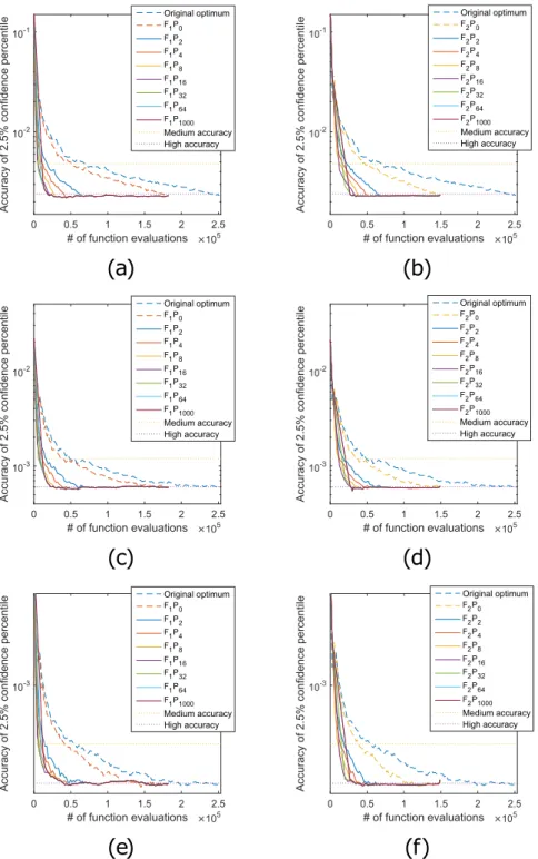
Bootstrap of a mixed model. In the previous paragraphs, we studied our methods by evaluating the number of function evaluations to find the optimum. However, the purpose of a resampling method such as the bootstrap is usually to compute an uncertainty measure (e.g., the standard error of an estimate or a confidence interval). In this result section, we will estimate the lower bound of a 95% confidence interval using the percentile bootstrap confidence interval method29_.

We will apply this bootstrap on a linear mixed model, a model commonly used in the life sciences9–13_.

The bootstrap of a linear mixed model is of interest in a variety of areas14,30–34_{, as inference for its random}

effects is not straightforward15–17_.

In this example we will use real-life data from Bringmann et al14_{. As stated in the introduction, 129}

depressed patients are measured repeatedly 10 times a day for 10 days using the experience sampling method regarding their momentary sadness35_{. As not all patients respond to every measurement, the data}

are unbalanced and consists of only 9115 time points. For each patient, sadness at timepoint t will be predicted by sadness at timepoint t−1. Both the intercept and the slope are assumed to vary across patients. We will use the bootstrap with B=2000 bootstrap iterations to estimate the 2 5 percentile of . %

the variance matrix of these random effects:

σ σ

σ σ

=   



 

. ( )

, ,

, ,

D

11

D D

D D

1 2

12

12 22

The more bootstrap samples are processed, the higher the accuracy of this 2 5 percentiles will . %

become. However, more bootstrap iterations generally means more function evaluations to estimate the mixed model parameters. Hence, there is an intrinsic trade-off between speed (number of function eval-uations) and accuracy. Next, we can study how the different options and variants of our method deal with this speed-accuracy trade-off. Option 1, taking naive starting values, will not be considered. All speed ups will be measured against option 2, taking the original optimum as starting value. Moreover, new variants will be introduced.

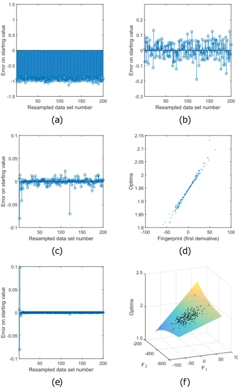
Figure 3. Choosing optimal starting values for a linear regression. A linear regression data set with estimated slope (the original optimum), βˆ0= .1 94, is non-parametrically resampled B=200 times. In this figure, the possible choices of the starting values for the optimization of the loglikelihood of these resample data sets are compared in (a–c) and (e). In all those panels the horizontal axis shows the resampled data set number b and the vertical axis the initial errors on the starting values Eb=θb−θˆb. In (a), a naive starting

value is chosen (βb=1, option 1). All errors are negative. In (b), the original optimum is chosen as starting value (option 2) which removes the bias. In (c), the results of the interpolation variant of option 3, using a one dimensional fingerprint (first order derivative) are shown (variant F1). Eb further decreases, but not to

machine precision. The reason is shown in (d): there is no unique relation between fingerprints 1 1, to

1 200, and optima βˆ1 to βˆ200. Data sets with the same fingerprint can result in different optima. In (e), the initial error Eb again decreases to zero. Here a two dimensional fingerprint, i={1,i,2,i}, using the first

and second-order of differentiation of the loglikelihood, is used (variant F2). This results in a unique, non-linear relation between the fingerprints and the optima, as is seen in (f), showing fingerprints (1 1,,2 1,) to

 

p refers to the ratio between the number of resampled data sets for which the optimization is bypassed compared to the number of resampled data sets for which the optimization algorithm is fully used. For example, if p is 3 and 200 bootstrap estimates are found with an optimization algorithm, then 600 pre-dicted estimates are added to create a total set of 800 estimates. However, the total number of estimates never exceeds 2000 (as we have B = 2000 bootstrap iterations). So with the different values of p, maxi-mum 200 predicted estimates will be added if already 1800 estimates are found with an optimization process. Note that the F P_g 0 variants are the same as the Fg variants of option 3, where the optimization

is never bypassed. All different options and variants are summarized in Table 1.

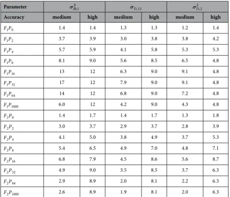
The resulting speed up is shown in Fig. 4 and Table 2. The accuracy is shown against the number of function evaluations, i.e. the computational burden. Our method can acquire the same accuracy up to 17 times as fast as the original optimum variant. More generally, for all the model parameters over all accuracies, approximately a tenfold speed up can be acquired. Using finite differences, more function evaluations are needed to generate a fingerprint that includes higher order derivatives. To get low quality predictions, a fingerprint of a lower order (F P1 _p) suffices. Therefore, it is faster to use only first order

derivatives when only a low accuracy of the 2 5 percentile is required. When a higher accuracy of this . % . %

2 5 percentile is required, it can be better to use more informative fingerprints, with higher order derivatives, to create better predictions. For parameters σ_D2_{,1 and σ}

,

D12 a fingerprint that uses only first

order derivatives is enough. For a medium as well as high accuracy, the F P1 _p variants outperform the

F P2 _p variants. However, for the third parameter, σD2,2, F P2 p is a better option when a high accuracy is

required. The better predictions now outweigh the extra cost of the larger fingerprint. It is also interesting to note that the F P_g 0 variant always gives the worst speed up. This means that, for this example, it is

always advantageous to bypass the optimization process for at least a part of the resampled data sets.

Bootstrap of a generalized extreme value model. As a second real-life application we will apply fingerprint bootstrapping on a generalized extreme value (GEV) distribution model36_{. Also for the}

infer-ence of GEV distributions, bootstrapping is a well-used tool37–40_{. Again we will estimate the lower bound}

of the 95% confidence interval of the parameters of the GEV distribution.

In De Kooy, The Netherlands, the maximum hourly mean windspeed was measured almost daily between 1906 and 201541_{. In total 39760 maxima where included. The GEV with one covariate (i.e., date}

of measurement) will be used to model these maxima. As explained in the method section, the estima-tion of this model leads to a four dimensional optimizaestima-tion problem, with parameters ξ (shape) , σ

(scale), α (intercept) and β (regression weight).

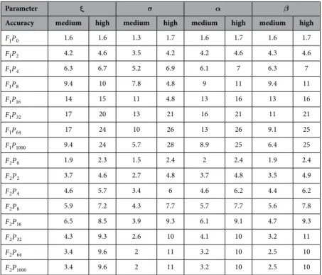
By counting the number of function evaluations needed to have a medium or high accuracy of the lower bound of the 95% confidence interval, we calculate the speed up of the fingerprint resampling method as shown in Table 3. The speed up of the F P_{g p} over the original optimum variation is even bigger as with the mixed model. The reason is that for the GEV distribution, using only the first derivatives of the likelihood as fingerprint, leads to sufficiently good prediction accuracies. Therefore, the F P1 p variants

can be used for the medium as well as the high accuracy. As the number of function evaluations needed to create the fingerprints of these F P1 p variants is significantly lower, the speed up is bigger. To achieve

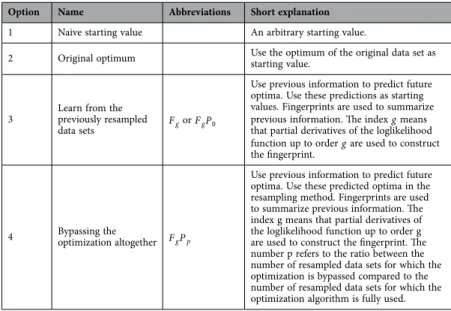
Option Name Abbreviations Short explanation

1 Naive starting value An arbitrary starting value.

2 Original optimum Use the optimum of the original data set as _{starting value.}

3 Learn from the previously resampled

data sets Fg or F Pg 0

Use previous information to predict future optima. Use these predictions as starting values. Fingerprints are used to summarize previous information. The index g means that partial derivatives of the loglikelihood function up to order g are used to construct the fingerprint.

4 Bypassing the _{optimization altogether} F Pg p

Use previous information to predict future optima. Use these predicted optima in the resampling method. Fingerprints are used to summarize previous information. The index g means that partial derivatives of the loglikelihood function up to order g are used to construct the fingerprint. The number p refers to the ratio between the number of resampled data sets for which the optimization is bypassed compared to the number of resampled data sets for which the optimization algorithm is fully used.

Figure 4. Trade off between accuracy and speed for the bootstrap of a mixed model. M=99 times, a mixed model is bootstrapped to compute the 2 5 percentile of the random effect variance parameters σ. % D2,1, σD,12 and σD2,2. Each bootstrap has B=2000 bootstrap iterations. On each panel, the error of this 2 5 . % percentile averaged over the M bootstrap processes, measured as described in the method section, is shown on the vertical axis. The average speed, measured in number of function evaluations, is shown on the horizontal axis. On the left panels (in (a), (c) and (e)), the results for variants F P1 p are shown, using only

a high accuracy in the lower bound of the 95% confidence interval, a speed up of about 25 is acquired for all the variables for the F P1 1000 variants. For the F P2 1000 variants again a speed up of about 10 is

reached. For the medium accuracies the F P1 p variants lead to speed ups around 10. Again, the F P2 p

variants do not perform very well when only a medium accuracy is needed. Too much time is needed to compute the detailed fingerprints, while only a medium accuracy is required.

Effect of parallelization on the speed up. Resampling methods earn part of their popularity by the fact they can be computed easily in parallel. Note that this parallel computing is no problem for our speed up. Only if literally every resampled dataset is handled simultaneously on a different computational entity, our speed increase will vanish. As long as parts of the resampling method stay serial, one can learn from previous information and consequently enjoy a speed increase. This is clearly shown in Fig. 5 for the GEV example. Here we show the speed up factor of the F P1 1000 variant while reaching a high

accu-racy. When everything is run on 1 core, we have a speed up of about 25 for every parameter. When more and more cores are used, the speed up decreases. When 2000 cores are used, every core computes one bootstrap. In this case, nothing can be learned from previous bootstrap computations. The speed up factor is now even below one, our method is slower as the normal method as the fingerprint resampling needs time to compute the fingerprints. If 5 cores are used (normal desktop computer), the method still enjoys 97% of the maximum speed up. When 20 cores are used, as is possible on a very high-end scien-tific computer, the method can reach 90% of the maximum speed up. On a supercomputer, using 100 cores, 47% of the speed up is preserved.

Discussion

The computational burden of resampling methods is oftentimes very large. Clearly, our fingerprint res-ampling method can decrease the computational cost enormously. The starting point of the fingerprint resampling is that in a resampling scheme, similar computations are done over and over again for very similar data. Ignoring the previous calculations would be a waste of time. By interpolating between structured previous information, predicting future optima and omitting the optimization process, we succeed in increasing the speed approximately by a factor of 10. We have illustrated our method with

Parameter σD2,1 σD,12 σD2,2

Accuracy medium high medium high medium high

F P1 0 1.4 1.4 1.3 1.3 1.2 1.4

F P1 2 3.7 3.9 3.0 3.8 3.8 4.2

F P1 4 5.7 5.9 4.1 5.8 5.3 5.3

F P1 8 8.1 9.0 5.6 8.5 6.5 4.8

F P1 16 13 12 6.3 9.0 9.1 4.8

F P1 32 17 12 7.9 9.0 9.1 4.8

F P1 64 14 12 6.8 9.0 7.2 4.8

F P1 1000 6.0 12 4.2 9.0 4.3 4.8

F P2 0 1.4 1.7 1.4 1.7 1.3 1.8

F P2 2 3.0 3.7 2.9 3.7 2.8 3.9

F P2 4 4.1 5.0 3.8 4.9 3.7 5.3

F P2 8 5.4 6.5 4.9 7.0 4.8 7.1

F P2 16 6.8 7.9 4.5 8.6 5.6 8.7

F P2 32 4.9 9.0 3.5 8.5 3.7 6.3

F P2 64 2.9 8.9 2.0 8.1 2.2 6.3

F P2 1000 2.6 8.9 1.9 8.1 2.0 6.3

Table 2. Speed up results for the bootstrap of a mixed model. The table shows how much faster the different variants, F Pg p, get at a high accuracy (approximately the lowest error achieved by the original

optimum variant) and a medium accuracy (approximately twice this error). These accuracies are shown in Fig. 4. Results are shown for the 3 parameters of D: σD2,1, σD,12 and σD2,2. The F Pg p variants are up to 17 times

faster as the original optimum variant. More generally, for all the model parameters over the majority of the accuracies, one can always find a F Pg p variant that leads to an 8 to 17 times faster bootstrap compared to

two simple examples but also with two real-life applications. The bootstrap of the mixed model can now be finished during a coffee break (20 minutes), while it took half a work day before (more than 4 hours).

In this paper, our method is proposed in such a way that it can be used for a broad range of resam-pling techniques. It can however easily be adapted to create a custom-made solution, increasing its effec-tiveness for more specific problems. For example, if the α% percentile has to be computed with a bootstrap, one can actually use a more advantageous, but more specific scheme. One can predict which resampled data sets are included in the < 2α% interval with fingerprints and then use an optimization

Parameter ξ σ α β

Accuracy medium high medium high medium high medium high

F P1 0 1.6 1.6 1.3 1.7 1.6 1.7 1.6 1.7

F P1 2 4.2 4.6 3.5 4.2 4.2 4.6 4.3 4.6

F P1 4 6.3 6.7 5.2 6.9 6.1 7 6.3 7

F P1 8 9.4 10 7.8 4.8 9 11 9.4 11

F P1 16 14 15 11 4.8 13 16 13 16

F P1 32 17 20 13 21 16 21 11 21

F P1 64 17 24 10 26 13 26 9.1 25

F P1 1000 9.4 24 5.7 28 8.9 25 6.4 25

F P2 0 1.9 2.3 1.5 2.4 2 2.4 1.9 2.4

F P2 2 3.7 4.6 2.7 4.8 3.7 4.8 3.5 4.9

F P2 4 4.6 5.7 3.4 6 4.6 6.2 4.4 6.2

F P2 8 5.9 7.2 4.3 7.7 5.7 7.7 5.6 7.8

F P2 16 6.5 8.5 3.9 9.3 6.1 9.1 4.7 9.3

F P2 32 4.3 9.3 2.6 10 4.1 10 3.2 11

F P2 64 3.4 9.6 2 11 3.2 10 2.5 10

F P2 1000 3.4 9.6 2 11 3.2 10 2.5 10

Table 3. Speed up results for the bootstrap of a GEV distribution. The table shows how much faster the different variants, F P_{g p}, get at a high accuracy (approximately the lowest error achieved by the original optimum variant) and a medium accuracy (approximately twice this error). Results are shown for the 4 parameters of the GEV: ξ, σ, α and β. The F P_{g p} variants are up to 28 times faster as the original optimum variant. More generally, for all the model parameters over the majority of the accuracies, one can always find a F P_{g p} variant that leads to a 24 times faster bootstrap, compared to the original optimum variant.

algorithm to find the real optima of these data sets. Using such a scheme, there is almost no error intro-duced while retaining the computational advantage. In another example, a Newton-Raphson optimiza-tion may be used. In such a case our method can easily be combined with k-step method of Davidson et al.21_{. One can first do a raw prediction of the optimum and can then refine this optimum with k}

optimi-zation steps.

Resampling methods earn part of their popularity by the fact they can be computed easily in parallel. Note that this parallel computing is no problem for our speed up. Only if literally every resampled dataset is handled simultaneously on a different computational entity, our speed increase will vanish. As long as parts of the resampling method stay serial, one can learn from previous information and consequently enjoy a speed increase.

Not all aspects of our fingerprint resampling method are known at this point. We discuss two of them. First, in the simulations of this paper, we treated all problems as local optimization problems. Problems with multiple local minima form however an even greater computational problem. Therefore we will address this problem in future research. Fingerprints may still be able to point in the right direction of the optima. The relation between the fingerprints and optima may however become very unsmooth if different resampled data sets converge to other kinds of minima.

Second, the final goal of most resampling techniques is to compute an uncertainty measure. It stays however unclear how much error is introduced in this uncertainty measure by predicting a certain amount of optima (the ratio p). Most black-box techniques can provide reliable prediction errors of the optima themselves, but it can be hard to translate those prediction errors to errors in the uncertainty measure. On the other hand, this is not a problem specific to our method. When our speed up is not used whatsoever, one still has to assign the accuracy of the optimization for every resampled data set. Moreover, most resampling techniques introduce errors themselves. For example, one can never exactly know the error that is introduced by only computing a limited number of bootstraps29_{. Future research}

has to assess how all these errors are combined in the final uncertainty measure.

In conclusion, the fingerprint resampling method presented in this paper may fuel a more widespread use of resampling methods for complex models, which is now impossible or difficult because of the large computational burden.

Methods

A general description of the fingerprint resampling method. The basic idea of our method was explained in the result section. In this section we will develop our method in a more systematical fashion and indicate that it can be used more generally. For simplicity and completeness, we will consider the same four options as in the result section. However, only the third and fourth options are variants of our fingerprint resampling method.

Option 1: A naive starting value. Starting values are very important for optimization algorithms. They greatly define the speed in which the optimization process converges. In practice, when little information is known about the estimation process, naive starting values can be used (such as zero, one, the unity matrix, etc.). Such a naive starting value may be biased in the sense that it is systematically too high or too low compared to the real optima of the resampled data sets.

Option 2: The original optimum θ^

0 as a starting point. Taking the original optimum, θˆ0, may lead to a

serious improvement over a naive starting value. As the original data set is central to the resampled data sets, the original optimum is likely to be central compared to the optima of the resampled data sets.

In the context of bootstrapping, the estimated bias on an estimator θˆ is calculated by

θ θ

= ∑

− , ( )

=

bias

B 12

bB 1 b

0

with ( ,..., )θˆ1 θˆB the B optima of the resampled data sets29. Assuming this estimated bias is zero, one has

θˆ = ∑ =θˆ . _{( )}

B 13

bB b

0 1

This means that the original optimum is exactly the mean of the bootstrap optima. As a consequence, if the estimated bias of the estimator θˆ is zero, the bias of θˆ₀ as a predictor for the optima of the resampled data sets, is also zero. Therefore, when no further information is known about a problem, this original optimum is usually a reasonably good initial value for the subsequent optimizations and it is easy to implement. Using the original optimum as initial value is the most unsophisticated way of using previous information and it is not unique to our procedure19–21_{. It may already lead to a significant speed increase}

Option 3: Learn from the previously resampled data sets. In a next phase we will try to create better predictions for the optima of a new resampled data set making use of the previously resampled data and their corresponding optima. The better the prediction, the better the starting value and the less iterations the optimization procedure needs. For this prediction, we need two ingredients. A first ingredient is a concise summary of the data sets into statistics, called fingerprints, which can be linked to the optima of the resampled data. As a second ingredient, we need a method that can be used to learn the relation between the fingerprints and the optima of past data sets.

It is clear that, in order for our method to be efficient, both the fingerprints and the method to learn the relation should place a minimal computational burden on the whole resampling calculation. In the following parts, we will discuss both ingredients. To conclude, we discuss the link with the tuning param-eters of the optimization algorithm.

Fingerprints. A fingerprint  is a scalar-valued or vector-valued function taking the resampled data set as input and produces one or more statistics as output. (In what follows, we will denote both the function as well as the function values with the term fingerprint.) To use such a fingerprint for the pre-diction of the optimum, it must contain information on this optimum in a parsimonious manner. Obviously, there is a trade-off between compression rate and retained information. For instance, a trivial fingerprint would be the identity function, which maps a data set onto itself. Such a fingerprint obviously contains all the necessary information to locate the optimum. However, the relation between the finger-prints and the optima is harder to derive when the fingerprint has a high dimensionality. Therefore, the identity function does not qualify as a good fingerprint because there is no information reduction.

The question then becomes what constitutes a good fingerprint. A derivative-based fingerprint is intuitively attractive. The rationale behind a derivative-based fingerprint is that the information con-tained in derivatives (rate of change, curvature, etc.) in a point near a local optimum will tell us some-thing about the location of the local optimum itself. In fact, the same kind of information is used in several optimization algorithms (e.g., steepest descent and Newton-Raphson). Therefore, we propose to use the derivatives of the objective function of the resampled data set, evaluated in the original optimum, as a fingerprint. Formally, this can be written as follows in the case of maximum likelihood estimation (for a particular resampled data set X_b):

_b= ∇ ({  θˆ ;X_b), ∇ ( θˆ ;X_b),...,∇ (g θˆ ;X ) ,} ( )14

b

0 2 0 0

where g is the order up to which the partial derivatives are used. (In case of least squares estimation  can be replaced by a sum of squares loss function S.) Of course, only the unique elements of the partial derivatives are used for the fingerprint: For example, if g equals 2, these are the first order derivatives combined with the upper triangular elements of the Hessian matrix.

The derivatives can be approximated using finite differences if no analytical expressions exist. Obviously, a fingerprint using finite differences gives another incentive to reduce the dimensionality of the fingerprint. The higher the order of the derivative that needs to be estimated, the more function evaluations need to be computed. If k is the dimension of the optimum, one needs at least k+1 function evaluations if g=1 and k+ k k( + )₂ 1 +1 function evaluations if g=2 when finite differences are used.

A more fundamental reason to use derivative-based fingerprints is provided by Taylor’s theorem. If a function can be completely approximated by a Taylor series, all its information can be summarized in its derivatives evaluated in a certain point (e.g., the original optimum). Taking an infinite number of (par-tial) derivatives (g→ ∞) will then lead to a fingerprint with all information needed to uniquely define the optimum of its function. However, it is not necessary to describe the function one wants to optimize, nor its associated data set in statistics. Already in a very compact fingerprint a lot of information can be found about the optimum. As already mentioned, we propose to take a fingerprint with a dimension as low as possible, for modeling reasons. A limited number of derivatives, for example all first-order deriv-atives in combination with all the unique elements of the Hessian matrix, will suffice in many cases.

It should be noted that a good fingerprint for one model does not necessarily generalize to a good one in another model. Sometimes, the likelihood cannot be evaluated in the original optimum for some data sets (see e.g., the example on the generalized extreme value distribution in the method section), making it impossible to compute the derivatives. Moreover, other ways of summarizing data may work at least as good as the derivative-based fingerprints. For example, computing the moments of a data set can also lead to good results. The sample average in the first example on the exponential distribution would obviously be a good fingerprint. Another possibility is to use summary statistics as they are used in approximate Bayesian computing. It is even possible to automatically generate such summary statistics42_.

In any case, what constitutes a good fingerprint is very problem specific. A covariance is decisive for the optimum in a regression while it cannot be computed in the data set of an exponential distribution. In situations where one has specific prior knowledge about the model, one can use this information to create a better model-specific fingerprint.

predict the optima of subsequent resampled data sets. These predicted optima can then be used as start-ing points.

The modeling of the relation between fingerprints and optima should satisfy three requirements. First, the modeling should be fast to calculate. The main reason for the prediction of the optima and using these as starting values is to create a significant speed up in the optimization procedure. However, this gain would be wasted in case of a slow modeling procedure. Second, the modeling should be able to describe a nonlinear relation. One cannot expect to only find strictly linear relations between the fingerprints and the optima. Already in the second simple example in the result section (on regression), the relation between optima and fingerprints is nonlinear. Third, we prefer to choose a method which excels in prediction. Both support vector machines (SVM43_{) and multivariate adaptive regression splines}

(MARS28_{) are well known for their generalization quality, which lead to good predictions. For the SVM,}

we propose to use a specific adaptation, the least squares support vector machines (LS-SVM), which lead to a much faster modeling compared to traditional SVM26_{. Note that these methods create a multi-input}

single-output model. This means that one needs one model for every dimension of the parameter that needs to be optimized. Because every dimension of the fingerprint initially has the same importance regarding the predictions, they are all standardized to train the black-box model.

The black-box methods are versatile, flexible and fast to compute. However, there are two specific problems that need to be addressed before the methods can be applied efficiently: constraints and extrapolation.

A first problem that needs to be solved is that some estimation problems call for a constrained opti-mization. If a parameter is constrained, this can lead to a non-smooth fingerprint-optimum relation. As an illustration, consider Fig. 6 which can be compared to Fig. 3d in the result section. In both figures the fingerprints of a linear regression are plotted against optima. However, in Fig. 6, the optima are found with a constrained optimization (θ^>_{2). A situation is shown where the fingerprints below a value of}

-30 all result in a value of 2 of the parameter θ^_{. It can be seen that if the constraint is active, then for} multiple resampled data sets, different fingerprints will all lead to the same optima, θ^=_{2. When at the}

same time, other resampled data sets lead to an inactive constraint, those resampled data sets will lead to a different fingerprint optima relation. There are now two different relations between the fingerprints and the optima. As a result, the relation between fingerprints and the optima is non-smooth. A black-box technique may have a hard time to learn such a non-smooth relation. For such cases, we propose the following solution. First, the black-box technique is only be estimated with the optima which are not on the boundary. Second, if the black-box technique makes a prediction that violates the constraint, the prediction is adapted to the constraint value.

fingerprint, the minimum and maximum is searched. For the data sets corresponding with one or more extrema, the optima are computed first. In total, 2 data sets are prioritized, with k k the dimension of the fingerprint. Second, a fair number of purely random data sets (usually, k) are added and also for these data sets the optima are computed. Postponing the use of the predictions for these initial data sets ensures a stable model over a broad range of fingerprints. To find the optimum, the original optimum is used as a starting value in this initial phase.

Other tuning parameters. The speed of most optimization algorithms can be improved and controlled by tuning parameters (e.g., the initial step length in line search algorithms for gradient-based methods; the size of the initial simplex in the Nelder-Mead method). It can also be useful to control these tuning parameters based on previous optimizations. Important in this control problem is that the uncertainty associated with the starting value should not be neglected. If the starting value is of high quality (because the predicted optimum and the true optimum are close together), the optimization algorithm should ini-tially only search for an optimum in a small area around it. Otherwise, the advantage of a good starting value may disappear. The quality of the starting value can be extracted from the prediction error of the interpolator.

Option 4: Bypassing the optimization altogether. If more and more optima are computed, more and more information becomes available to train and improve the model that estimates the relation between the fingerprints and the corresponding optima. If both the fingerprints and the method to model this relation are chosen well, prediction errors of subsequent optima can become very small. When these predicted optima are used as starting values, the optimization process will only add little accuracy to the estimated optima. The starting values can become practically indistinguishable from the real optima. In such a case, it is not a problem to bypass the optimization process because the accuracy that can be gained is negligible compared to intrinsic (i.e., Monte Carlo) error in the resampling itself1,21_{. Therefore,}

it is unnecessary to know the optima with highest possible precision. The predicted optima, including a small error, can just as well be used as the real optima. This brings the speed increase of our method to a whole new level, the optimization process can now be skipped. As we note in the discussion, it can be hard to estimate how this prediction error exactly influences the accuracy of the uncertainty measure the resampling method computes.

Assessing the performance of the methods. The performance of the methods is assessed from two perspectives. First, the time needed to estimate the parameters for the series of resampled data sets (averaged over a number of replications in order to reduce the error) is evaluated. Second, we assess how the different methods deal with an intrinsic speed-accuracy trade-off: A longer computation time leads to more accurate results, but how does the accuracy of the methods compare given a fixed computational load?

We measure computation time in terms of number of function evaluations (where the function is the objective function that needs to be optimized for every resampled data set, such as the likelihood or least squares loss function). The two computationally most expensive parts of our method (i.e., the time the optimization algorithm needs to converge and the computation time of the derivative-based fingerprints) can be measured in this number of function evaluations.

The method proposed in this paper will be most useful if the optimization process is unbearably slow. Another aspect of our method involves the modeling of the relation between the fingerprints and the optima and does not place a large burden on the computation. It can be neglected because it does not scale with the difficulty of the optimization process. The relative amount of time needed for the interpo-lator (such as the LS-SVM or MARS) will be close to zero in cases of high computational burden. For example, using one core on an Intel Core i7-3770 with 3.4 GHz, the execution time of the estimation of one LS-SVM is 1.5 seconds with a training set of 200 previous fingerprints and optima.

Another reason not to consider the interpolator in the total computational cost is because it is unnec-essary to update the modeled relation between fingerprints and optima after each optimization process. The modeled relation and the quality of the predictions will only significantly change if the training data changes significantly. This will not be the case if only one couple (i.e., fingerprint and associated opti-mum) is added. We propose to update and remodel the relation only when 10 more information is %

available. In practice, the modeling of the relation can be stopped if the reduction in prediction error is only marginal. We stop this modeling when more than 1000 optima are found. Other machine learning improvements are possible to further reduce the time needed by this modeling, like online updating and big data solutions27_{. All these options are however not included to present a much cleaner picture of our}

method.

Optimization algorithm. The optimization procedure used by fingerprint resampling is not central to the method. In the result section we use the Nelder-Mead method44_{. This algorithm is used for its}

generality and its popularity45_{. It is derivative free and can be used on almost any convex function.}

Moreover, it is the default algorithm used by the basic optimizers in Matlab and R (i.e., fminsearch in Matlab46,47_{, and optim in R}48_{) and it is used in the popular lmer function in R to estimate mixed}

models. The Matlab function fminsearch is used as basic implementation of this algorithm.

The Nelder-Mead method is an optimization algorithm that uses simplexes with D+1 vertices V Vd VD

( ,₀ ,... ) , with D the dimension of the parameter vector to optimize. When initializing the algo-rithm, vertex V0 is set to the starting value, θ. For example, in the fminsearch function, the complete

initial simplex is then assigned similar as in Algorithm 1.

θ θ = = ( )=( + . ) ( )   V V

V d V d

for d from 1 to D do ;

1 0 05 ;

d

d d

0

Algorithm 1. Initialization of the initial simplex as done by fminsearch, for V d0( ) not equal to zero. ( )

V dd is the d-th entry of vector Vd.

The initial simplex can be improved upon considerably when more information becomes available. When modeling the relation between the fingerprints and the optima, future optima are predicted but we can also estimate an error of these predictions. For instance, this error can be estimated with a fast leave-one-out cross-validation. The interpolator will assign for dimension d of the parameter vector a prediction error, denoted ε( )d . The assignment of the initial simplex is then changed as indicated in Algorithm 2. θ θ ε = =

( ) = ( ) + ( ( ), θ)





V

V

V d V d max d Tolerance

;

for d from 1 to D do ;

d

d d

0

Algorithm 2. Initialization of the initial simplex using the prediction error ( )d for each dimension d.

( )

V d_d is the d-th entry of vector V_d. Toleranceθ is the user-defined value for assessing convergence

based on the parameter values.

The convergence criterion used for the Nelder-Mead optimization method is when the maximum distance (infinite norm) between the vertices is smaller than Toleranceθ and the maximum difference

between their corresponding function values is smaller than Tolerance_f. In our applications, both tol-erances are set to ₁₀−6_.

Mathematical models used. In the result section we make use of an exponential distribution, a linear regression, a mixed effects model and a generalized extreme value distribution. The mathematical model of the exponential distribution is already discussed in this result section. Here we will give every necessary detail about the other three models.

Linear regression. In the second simple example in the result section, a linear regression model is used. With data set X= ( , ), ( ,

(

)

like-lihood is given by

 β σ

∏

πσ β σ ( , ) =    − ( − )    . _{( )} =

X exp y x

; 1

2 2 15

i n i i 2 1 2 2 2

Its loglikelihood is given by

β σ πσ β β

σ

( , ) = − − ( − ) ( − ), _{( )}

 ;X n log y x y x

2 2 2 16

t

2 2

with x= ( , …,x1 xn)t and y= ( , …,y₁ y_n)t. For simplicity, only the case where σ2 is known and equal

to one is considered. The loglikelihood simplifies to

β π β β

( ) = − − ( − ) ( − ). _{( )}

 ;X n log y x y x

2 2 2 17

t

In the result section, M=99 synthetic data sets are simulated with n=100, β=2 and σ2=1_{. For} each simulated data set, B=1000 bootstrap data sets are generated. For each bootstrap sample this loglikelihood is maximized for the single parameter β. Its analytical solution is given by

βˆ = x y. _{( )}

x x 18

t t

As explained in the result section, an iterative optimization algorithm is used to optimize the loglikelihood.

For variant F1, a one-dimensional fingerprint is created using the first derivative of the loglikelihood

in the original optimum:

 β σ

β β = ( , ) = − + , ( ) β β , =  ˆ ˆ d X d

x y x x

; 2

2 ₁₉

b b b

t

b tb b

1

2 ₀

0

For variant F2, a two-dimensional fingerprint is created by combining this fingerprint with the second

order derivative of the loglikelihood in the original optimum:

 β σ

β

= ∂ ( , )

∂ _{β β} = . _{( )}

, =  ˆ X x x ; 20

b b tb b

2

2 2

2

0

Both derivatives are computed with finite differences in the result section. As shown in the result section, one cannot create an exact function between fingerprint 1,i from Equation 19 and the optimum

βˆ_i from Equation 18 (variant F1). However, using a two dimensional fingerprint (variant F2), using

Equations 18, 19 and 20 one can derive the following functional relation:

 



β = β − .

( )

, ,

,

ˆ ˆ

21

b b b

b

0 2 1

2

This relation leads to much better predictions of new optima, as is illustrated in the result section.

Mixed model. In line with Verbeke & Molenberghs8_{, we start with a random sample of N units. For}

each unit i, n_i measurements are taken with respect to an outcome variable and these measurements are collected in a vector y_i. Next, the following model is assumed:

β ε

=X +Z + . ( )

y_i i i ib i 22

with bi∼N( , )0 D and εi∼N( ,0 σ2I) and b1,..., , ,...,bN ε1 εN independent. The parameter vector β

contains the fixed effects regression coefficients and D is the population variance-covariance matrix. Such a general linear mixed model implies the following marginal model:

σ

β

∼ ( , + ), ( )

Y_i N X_i Z DZ_{i i}t 2I 23

The loglikelihood is then given by

∑

= − ( ( ( , ) ) + ( − ) ( , )( − ) + ( )), _{( )}

=

−

 2 log V Y X V Y X n log 2

24

i N

i D i i t i D i i i

1

1

with

σ σ

σ σ σ

σ σ σ σ σ σ σ ( , ) = ( ) + =        ... ... ... ... ... ... ... .... ...       + . ( ) , , , , , , ,

V Z D Z I Z Z I

25

i i it i

D D D m

D D

D m D m

i t

D D 2

1 2

12 1

12 22

1 2

2

decomposition of D49_{. Second, to reduce the number of parameters of the optimization problem, β and} σ can be profiled out50_{. This leaves us with unique} m m( + )1

2 parameters, θ= ( ,...,θ1 θm m( + )/1 2), to

opti-mize. To find the variances of random effects of the mixed model, the resulting optima (both the ones found after an iterative optimization and the ones predicted) have to be translated back to their original parametrization, as used in Equation 24. Note that, due to the Cholesky decomposition, some of these parameters can only have a positive contribution in Equation 24. For example, a parameter θ_i is only used as θ_i2, even when θ<0 it can only have a positive contribution θ2>0. This means that we introduce an indirect constraint.

In the data of Bringmann et al., used in the result section, both the intercept and the slope are assumed to vary across patients14_{. No restrictions are imposed on the variance matrix of these random}

effects (except for positive definiteness):

σ σ σ σ =       , ( ) , , , , D 26 D D D D 1 2 12

12 22

which leads to a three dimensional optimization problem.

To bootstrap this data, we use the so-called case bootstrap30,31_{. The case bootstrap is a non-parametric}

bootstrap which uses the clusters (in our case, the patients), as entities to sample from. The whole boot-strap process is repeated M=99 times, each time with B=2000 new random bootstrap iterations.

In the software package (see the Code availability paragraph), in the exampleFingerprintBootstrap.m file, the fingerprint bootstrap is also applied on a mixed model using artificial data.

Generalized extreme value distribution. For the generalized extreme value distribution with data set

= (( , ), ( , ),...,( , ))

X x y1 1 x y2 2 x y_{n n} , shape parameter ξ, scale parameter σ and location parameter µ_i=α+βxi, the likelihood is given by

 ξ σ α β

∏

σ ( , , , ) =   −   + − _   . ( ) ξ = − / X y

; exp 1

27 i n i i 1 1

In the data set used in the result section, x_i is given by the maximum windspeed of a certain day, and

y_i is given by the date (number of days after first measurement). The logarithm of this likelihood is computed using an adapted version of gevlik.m of Matlab46_{. To find the maximum of this loglikelihood,}

a four dimensional optimization problem is solved using the Nelder-Mead method. As a naive starting value we use moment estimators as proposed by Hosking et al.51 _{and a least squares estimation for the} α and β parameters52_.

It is interesting to note that the likelihood can only be computed if 1+ξyi−_σµi>0_{. It is therefore} possible that for some data sets, the fingerprint resampling method might need to be adapted. If the original optimum leads to an invalid likelihood for some bootstrap data sets, the original optimum can-not be used as a starting value, nor can the derivatives be calculated to create a fingerprint. In such a case, it is advised to use another sort of fingerprint. For the data set in the result section, there were no such problems.

Speed-accuracy trade-off for the bootstrap. In the result section, we estimate the lower bound of a 95% confidence interval using bootstrap. From a series of B bootstrap samples, this lower bound is the

. %

2 5 percentile, denoted as θˆ( .B0 025). Using the percentile bootstrap confidence interval method, this per-centile can be estimated as29_:

θˆ( .B0 025)= ( .{ 0 025⌊ B)⌋th largest of }θ^b, ( )28

where ⌊ ⌋⋅ is the flooring function. Obviously, it is always better to use more than less bootstrap itera-tions. For the mixed model problem we use B=2000 bootstrap iterations as the end goal. However, we also monitor θˆ( .b0 025) as a function of b= , , …,1 2 B. For any b or B< ∞, θˆ( .b0 025) and θˆ( .B0 025) will always be approximations of θˆ_{( .}∞_{0 025)}, which uses an infinite number of bootstrap iterations. Adding bootstrap optima one after the other, our estimate θˆ( .b0 025) will come closer and closer to θ( . )

∞

ˆ_{0 025}. The error will decrease further and further. However, more bootstrap iterations generally means more function evalu-ations. Hence, there is an intrinsic trade-off between speed (number of function evaluations) and accu-racy (|ε_{( .}b ₎|

0 025 , the absolute difference between θˆ( .b0 025) and θ( . ) ∞