Volume URL: Chapter Author: Robin L. Lumsdaine, James H. Stock, David A. Wise

Volume Title: Studies in the Economics of Aging

Volume Author/Editor: David A. Wise, editor

Volume Publisher: University of Chicago Press

Volume ISBN: 0-226-90294-3

Volume URL: http://www.nber.org/books/wise94-1

Conference Date: May 1992

Publication Date: January 1994

Chapter Title: Pension Plan Provisions and Retirement: Men and Women,

Medicare, and Models

Chapter Author: Robin L. Lumsdaine, James H. Stock, David A. Wise

Chapter URL: http://www.nber.org/chapters/c7344

Pension Plan Provisions and

Retirement: Men and Women,

Medicare, and Models

Robin L. Lumsdaine, James H. Stock, and David A. Wise

Our ongoing analysis of the effects of pension plan provisions on retirement is pursued in this paper. The work to date has emphasized the dramatic effect of employer-provided pension plan provisions on age of retirement and the enormous effects of changing the provisions. The work has also highlighted the important limitations of using Social Security provisions to predict retire- ment behavior, without accounting for the effect of employer pension plan pro- visions, which, for employees who have such plans, is typically much more powerful than the effect of Social Security provisions.

Two aspects of our work have guided the analysis as the research progressed. The first is that a new method has been used to model retirement decisions. The second is that the empirical analysis has been based on data from individ- ual firms. Thus we have been led to consider whether the model provided accu- rate predictions of the effects of plan provisions on retirement and whether the behavioral implications of analysis based on data from one firm could be generalized to other firms with different plan provisions.

In two initial papers, Stock and Wise (1990a, 1990b) developed an “option value” model of retirement. The central feature of this model is that in deciding whether to retire employees are assumed to compare the “value” of retiring now to the maximum of the expected values of retiring at all future retirement ages. If the maximum of the future values is greater than the value of retirement

Robin L. Lumsdaine is assistant professor of economics at Princeton University and a faculty research fellow of the National Bureau of Economic Research. James H. Stock is professor of political economy at the John E Kennedy School of Government, Harvard University, and a re- search associate of the National Bureau of Economic Research. David A. Wise is the John E

Stambaugh Professor of Political Economy at the John E Kennedy School of Government, Har- vard University, and the area director for Health and Retirement Programs at the National Bureau of Economic Research.

Financial support from the National Institute on Aging and the Hoover Institution (Wise) is gratefully acknowledged. The authors also thank Jim Smith and John Rust for helpful comments.

now, the employee continues to work. We tested the predictive validity of this model in two ways: first, we considered the “within-sample fit” of the model, by comparing the actual pattern of retirement by age to the pattern predicted by the model, based on the data used for estimation. Second, in papers by Lumsdaine, Stock, and Wise (1990, 1991) we emphasized an external “out- of-sample’’ check of predictive validity, by considering how well the model predicted the effect on retirement of an unanticipated and temporary change in the pension plan provisions, occasioned by an early retirement window plan. In a subsequent paper, Lumsdaine, Stock, and Wise (1992) compared the pre- dictive validity of the option value model with that of two versions of stochastic dynamic programming models. The stochastic dynamic programming model is close in spirit to the option value model, but the prediction of retirement is based on the comparison of the value of retirement now to the expected value

of the maximum of the values of future retirement ages. The evidence was that the option value model predicted just as well as the stochastic dynamic programming models, but had the advantage of being much less complex nu- merically. Ausink (1991) pursued a similar comparison based on retirement from the military and found that the option value version was noticeably better than the stochastic dynamic programming versions.

All of these papers, with the exception of the work by Ausink, are based on data from a single firm. The use of firm data was motivated by the absence of information on pension plan provisions in standard data sources, such as the Retirement History Survey, and by the realization that the incentives inherent in such plans could be very substantial and varied widely among firms, as shown in papers by Bulow (1981), Lazear (1983), and Kotlikoff and Wise (1985, 1987, 1988). In principle, the ideal data source would provide retire- ment information and pension plan information for a random sample of em- ployees, from a wide range of firms. Such information has not been available. The alternative we followed was to obtain data from several different firms. The hope was that similar results from different firms would tend to confirm the validity of the model, even though the firms themselves could not be con- sidered a random sample of all firms. Thus there is a need to determine whether the results for the single firm are confirmed based on data from other firms.

Therefore, the first goal of this paper is to use data from a new firm to con- firm that the age pattern of retirement corresponds to the pension plan provis- ions. Descriptive analysis confirms that this is the case.

A second emphasis in this paper is the comparison of the retirement behav- ior of men and women. It is sometimes proposed that women may tend to retire earlier than men because they are typically younger than their husbands and they may tend to retire when their husbands do. From descriptive analysis, it is clear that the retirement patterns of men and women are not appreciably dif- ferent.

A third goal is to add another observation to the list of comparisons of the predictive validity of the option value versus that of the stochastic dynamic

185 Pension Plan Provisions and Retirement

programming model. Predictive validity in this paper is judged by the model predictions of retirement under a special 1983 early retirement incentive plan. The models are estimated based on retirement decisions in 1982. The goal of the comparisons is to accumulate data on the extent to which the different models predict actual retirement choices and thus to determine which specifi- cation best approximates the considerations that determine actual retirement decisions. The emphasis is not on which model best approximates the econo- mists’ view of the “right” calculation, but rather which best approximates the calculations that the typical person makes. Or, better still, which predicts best the retirement decisions of the typical employee.

A fourth goal is to make limited inferences about the potential effect of Medicare availability on retirement, especially at age 65. We have found in our previous work that model predictions of the age-65 retirement rate are typi- cally much lower than the actual rate. We have attributed the high actual rate to an “age-65 retirement effect.” But our work, and we believe the work of others, has ignored the potential effect of Medicare insurance that becomes available at age 65. The approach used here is to consider how retirement rates-especially at age 65-would be affected were Medicare valued ac- cording to the average payments to the covered population. The final goal is to compare parameter estimates based on data from two firms with different pension plans.’

6.1 Background

6.1.1 The Firm I11 Plan

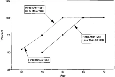
Employees are covered by a defined-benefit pension plan with normal retire- ment at age 65 and early retirement at age 5 5 . Cliff vesting occurs at 10 years of service (YOS) or at age 65, whichever comes first. The normal retirement benefit at 65 depends on earnings, age, and years of service at retirement (that is, at the time of departure from the firm). A person can retire and elect to start receiving benefits before age 65, but the normal benefit will be reduced by 5 percent for each year that receipt of benefits precedes age 65, as shown in figure 6.1. A person who retired at age 5 5 , for example, would receive 50 percent of the normal retirement benefit of a person who left the firm at age 65. (The normal benefit also depends on years of service at the time of retire- ment.)

However, if a person has 30 years of service at retirement and if the person is age 60 or older, the person is eligible for 100 percent of the normal benefit. Benefits are reduced 5 percent for each year that retirement precedes age 60,

I. In order to maintain numerical consistency throughout our work, we refer to the firm used in this analysis as ‘‘firm 111.’’ The comparison firm, used in Stock and Wise (1990a, 1990b) and Lums- daine, et al. (1990, 1991, 1992), is “firm I.”

1 w- 75- 50- Hired After 1951 30 or More YOS \

Less Than 30 YOS

25

'

1 I I

50 55 60 65 70

Age

Fig. 6.1 Early retirement benefit ( % of normal age-65 benefit)

if the person has 30 years of service. For example, a person who retired at age 55 with 30 years of service would receive 7 5 percent of the normal benefit.

Even a person who retires before age 55 and is vested can elect to receive benefits from the pension plan as early as age 55, but like the post-55 retiree, benefits are reduced 5 percent for each year that receipt of the benefits precedes age 65. Of course, this person's benefits would be based on earnings, age, and years of service at the time of retirement, unadjusted for earnings inflation, and would thus be lower than the benefits of a person who retired later.

Employees who joined the firm before 1951 can retire as early as age 50 and begin to receive benefits immediately, but at a reduced rate. An employee hired before 1951 had at least 31 years of service in 1982. The reduction for this group is indicated by the extended line that indicates benefits at age 50 to be 54.3 percent of the age-60 benefits for an employee who has 30 or more years of service at retirement.

To understand the effect of the pension plan provisions, figure 6.2A shows the expected future compensation of a person from our sample who is 5 1 years old and has been employed by the firm for 23 years. To compute the data graphed in figures 6.2A-6.20, a 5 percent real discount rate and a 6 percent inflation rate are assumed. The discount rate is estimated in the empirical anal- ysis, and the inflation rate is assumed to be 6 percent. Total compensation from the firm can be viewed as the sum of wage earnings, the accrual of pension benefits, and the accrual of Social Security benefits. (This omits medical and other unobserved benefits that should be included as compensation, but for which we have no data.) As compensation for working another year, the em-

I O J C , I , 1 I I , I , , I 7-m I I I I ~- I r J 51 52 53 54 55 56 57 50 59 50 61 62 63 64 65 66 67 58 69 70

I /

C 7 M ~ I 6 0 0 1 un 300 m IW

Age of Retirement Age of Retirement

O ' J , , , , , r 1 1 I I

'

€0 61 62 63 64 65 66 67 58 69 10 Age of Retirement 0' J I €4 65 66 67 58 69 70 Age of Retirement + Pension + Psn+SS 8 T o t a m p Fig. 6.2

age 64 with 45 YOS

ployee receives salary earnings. Compensation is also received in the form of future pension benefits. The annual compensation in this form is the change in the present value of the future pension benefits entitlement, due to working an additional year. This accrual is comparable to wage earnings. The accrual of Social Security benefits may be calculated in a similar manner, and is also comparable to wage earnings. Figure 6.2A shows the present value at age 5 I of expected future compensation in all three forms. Wage earnings represents cumulated earnings, by age of retirement from the firm (more precisely, by age of departure from the firm, since some workers might continue to work in another job). For example, the cumulated wage earnings of this employee be- tween age 5 1 and age 60, were he to retire at age 60, would be about $482,000, discounted to age-51 dollars. The slope of the wage earnings line represents annual earnings discounted to age-5 1 dollars,

The pension line shows the accrual of firm pension benefits, again dis- counted to age-5 1 dollars. The shape of this profile is determined by the pen- sion plan provisions. The present value of accrued pension benefit entitlements at age 5 1 is about $54,000. The present value of retirement benefits increases between ages 51 and 57 because years of service and nominal earnings in- crease. An employee could leave the firm at age 53, for example. If he were to do that and if he were vested in the firm’s pension plan, he would be entitled to normal retirement pension benefits at age 65, based on his years of service and nominal dollar earnings at age 53. He could choose to start receiving bene- fits as early as age 55, the pension early retirement age, but the benefit amount would be reduced 5 percent for each year that the receipt of benefits preceded age 65. Because 5 percent is less than the actuarially fair discount rate, the present value of benefits of a person who leaves the firm before age 55 are always greatest if receipt of benefits begins at 55.

Recall that a person who has accumulated 30 years of service and is 55 or older is entitled to increased retirement benefits that would reach 100 percent of normal retirement benefits at age 60. No early retirement reduction is ap- plied to benefits if they are taken then. So a person at age 60 with 30 years of service who continues to work will no longer gain 5 percent a year from fewer years of early retirement reduction, as occurs before age 60. There is a jump in the benefits of a person younger than 60 who attains 30 years of service. That accounts for the jump in the benefits of the person depicted in the figure 6 2 4 , when he attains 30 years of service at age 58.

The Social Security (SS) accrual profile is determined by the Social Security benefit provisions. The present value of accrued Social Security benefit entitle- ments at age 51 is about $33,000. Social Security benefits cannot begin until age 62. If real earnings do not change much between ages 5 1 and 62, then real Social Security benefits at age 62 will not change much either. After age 62, the actuarial adjustment is such that the present value of benefits, evaluated at the age of retirement, does not depend on the retirement age. But the present value of the benefits discounted to the same age (51 in this case) declines.

189 Pension Plan Provisions and Retirement

There is a further drop after age 65, because the actuarial adjustment is reduced from 7 percent to 3 percent.

The top line (Tot comp) shows total compensation. For example, the wage earnings of an employee who left the firm at age 60 would increase $482,000 between ages 5 1 and 60, shown by the wage earnings line. Thereafter, the em- ployee would receive firm pension plan and Social Security retirement benefits with a present value-at age 51-of about $170,000. The sum of the two is about $652,000, shown by the top line. Compared to total compensation of $575,000 between ages 5 1 and 60, an average of $63,000 per year, total com- pensation between ages 60 and 65 would be only $100,000, or $23,000 per year. Thus the monetary reward for continued work declines dramatically with age.

Figures 6.2B-6.20 show comparable compensation profiles for employees who are ages 57, 60, and 64, respectively, in 1982; they have 29, 38, and 45 years of service, respectively. The person depicted in figure 6.2B attains 30 years of service at age 58; thus the jump in pension benefits at that age. The present value of pension plus Social Security compensation (Pen

+

SS) reaches a maximum at age 59 and declines thereafter. Were this employee to continue to work after age 59, until 65, the present value of total retirement benefits would fall by $33,000, offsetting about 28 percent of the present value of wage earnings over this period ($117,000). A similar prospect faces the employee depicted in figure 6.2C but this employee is already entitled to 100 percent of normal retirement benefits and loses benefits for each year that he continues to work.

The employee who faces the figure 6.20 compensation profile is 64 years old and loses both pension and Social Security benefits for each year that re- tirement is postponed. At age 65, for example, about 54 percent of expected wage earnings would be offset by a reduction in retirement benefits, if retire- ment were postponed.

6.1.2 The 1983 Window

Under the window plan, which was in effect from January 1 to February 28, 1983, all employees were eligible for a separation bonus, but the most gener- ous payments were available to persons age 55 and older who had at least 21 years of service. Retirement benefits for this group were increased depending on age and years of service. For example, a person age 59 with 28 years of service could receive 100 percent of normal retirement benefits, instead of 70 percent under the regular plan. That is, this person’s retirement benefit would be increased by 43 percent. A person who was age 55 with 2 1 years of service could receive 55 percent of the normal benefits, instead of 50 percent. Persons age 60 or older with 30 years of service were eligible for 100 percent of normal benefits under the regular plan.

In addition, all employees were eligible for a separation bonus equal to one week’s pay for every year of service, with a minimum of 2 weeks and a maxi-

mum of 26 weeks of pay. Thus even persons who were under 55 and those who were eligible for 100 percent of normal retirement benefits faced an added inducement to retire.

6.1.3 The Data

The data used in the analysis are drawn from the personnel records of all persons employed by the firm at any time between 1979 and 1988. A year-end file is available for each year. Earnings records back to 1979 (or to the date of hire, if after 1979) are available for each employee. In addition, the data contain some demographic information, such as date of birth, gender, marital status, and occupational group. The retirement date of employees who retire is also known. (More generally, the date of any departure is known, and the reason for the departure is recorded.) Thus we are able to determine whether a person who was employed at age a was also employed at age a

+

1, and if not, the exact age at which the employee left the firm.

The estimation of the retirement model in this paper is based on 1982 data, whether or not an employee left the firm in 1982. (To simplify the determina- tion of age of retirement, only employees born in January and February and who had not retired before March 1, 1982, are used in this analysis.) The pri- mary test of the predictive validity of the model is based on how well the model, estimated on 1982 data, predicts retirement under the 1983 window plan that substantially increased standard retirement benefits.

6.2 Departure Rates for Men versus Women 6.2.1 Life-Cycle Departure Rates

Firm departure rates for employees aged 20-70 are shown in figure 6.3. The graph reflects average departure rates over the years 1979-82. After substantial turnover at younger ages, annual departure rates fall continuously to 1-2 per- cent at ages 45-54. Employees start to leave the firm in larger numbers at age 55, the early retirement age.

Figures 6.4A-6.4C compare the departure rates for men and women. Figure 6.4A pertains to employees with less than 10 years of service, who are not vested in the firm’s pension plan. Figure 6.4B pertains to employees with 10- 29 years of service, and figure 6.4C to those with 30 or more years of service. The striking aspect of the graphs is that there is virtually no difference between the departure rates of men and women, except at the principle child-bearing ages-say, 23 to 37. For example, between ages 37 and 54 the turnover rates of men and women with 10-29 years of service are almost identical. Among employees with less than 10 years of service, there is little difference in the departure rates of men and women between ages 37 and 65. Men and women with 30 or more years of service have almost identical departure rates at all ages.

191 Pension Plan Provisions and Retirement

0 ' , ,,, ,,, ,,, ,I I I , , I , I I , I I I , I I I I I I I I

2b'

' ' '25' ' ' '30' ' '35 40 45 50 55 60 65 70 Age

Fig. 6.3 Departure rates by age: men and women together

6.2.2 Retirement-Age Departure Rates

The departure rates for persons aged 50 and above are shown in figure 6.5 for men and women. These rates are based on 1982 data only. There is a notice- able increase in departure rates at age 55, from less than 1 percent for persons 50-54 years old to 3 or 4 percent for employees 55-59 years old. Although the increase in the annual departure may seem small, the cumulative effect of the increase is substantial. For example, with a 4 percent annual departure rate, 19 percent of persons in the firm at age 54 will leave before age 60. At a 1 percent annual rate, only 5 percent will leave.

There is also a sharp increase at age 60, the age at which persons with 30 years of service are entitled to 100 percent of normal (age-65) benefits. The sharp increases at ages 62 and 65 correspond to the Social Security early and normal retirement ages.

The plan provisions suggest that for employees age 55-64, and especially those 55-60 or 61, the departure rate for persons with 30 or more years of service should be higher than the rate for persons with less than 30 years of service. The descriptive data are shown in figure 6.6. The departure rates for men with 30 or more years of service are higher in the 55-61 age range. They are also higher for women at age 60, but the differences at other ages are small. Women with less than 30 years of service appear more likely than men to take early retirement between the ages of 55 and 6 1.

These data also reveal what may be an individual-specific work effect. Em- ployees with 30 or more years of service who have not retired before age 65 are

7

A 0 8 1

-~

- Men - - - Women1 ,-.._...- ... ,-..-Vv' 20 "25' 'I'Jo' ' "3b' ' 4 0 ' " 4 5 ' ' "50' ' " 5 5 ' ' '60' ' ' ' 6 5 ' 7b F X i F --- Women C 0 4 5 0 4 - 0 3 5 - h n x T 5 " 40 ' ' 4 5 ' " Age 1 - Men Women

1

L

Fig. 6.4 Departure rates by age: men and women (A) with less that 10 YOS,

193 Pension Plan Provisions and Retirement

+- Men 1982 + Women 1982

Fig. 6.5 Departure rates: men and women compared, 1982

a) c

d

0.36

2

n ?! 0.24 aJ Age

thereafter less likely to retire than employees with less than 30 years of service. In summary: even without formal analysis, the graphs make it clear that the pattern of departures reflects the provisions of the pension plan. The pattern is also consistent with Social Security provisions, but the magnitude of the age- 65 departure rate seems much more abrupt than the reduction in Social Secu- rity benefits at age 65 would suggest. These graphs also make it clear that there is little appreciable difference between the retirement patterns of men and women, with the possible exception of a greater likelihood of early retire- ment for women with less than 30 years of service. But in general, there is no evidence of a substantial difference in the retirement patterns of men and women.

6.2.3 Window-Plan Retirement Rates

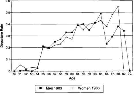
Departure rates under the 1983 window plan are shown for men in figure 6.7A and for women in figure 6.7B. These rates are contrasted with the average 1982 rates, shown on the same graph. Departure rates under the window plan were typically three to five times as large as the 1982 rates. Like 1982 depar- tures, there was little difference in the departure rates of men and women under the window plan, as shown in figure 6.8. There is, however, some indication that women under age 55 may have been more likely than men to accept the separation bonus.

6.3 Formal Models and Prediction of Retirement 6.3.1 Models

Two models are compared during the course of the analysis: the “option value” model and a stochastic dynamic programming model. Both are de- scribed in Lumsdaine et al. (1992), and excerpts from that paper are included as an appendix to this chapter. The models are explained only briefly here.

The Option Value Model

At any given age, based on information available at that age, it is assumed that an employee compares the expected present value of retiring at that age with the value of retiring at each age in the future through age 74. The maxi- mum of the expected present values of retiring at each future age, minus the expected present value of immediate retirement, is called the option value of postponing retirement. A person who does not retire this year maintains the option of retiring at a more advantageous age later on. If the option value is positive, the person continues to work; otherwise she retires. With reference to figure 6.1, for example, at age 5 1 the employee would compare the value of the retirement benefits that she would receive were she to retire then-approxi- mately $87,000-with the value of wage earnings and retirement benefits in

195 Pension Plan Provisions and Retirement 50 51 52 53 54 55 53 57 58 59 €0 61 62 63 64 65 66 67 66 69 70 Age B

B

c

6

1

+- Men 1982 -+- Men 1983

I

" " 0 5 0 4 0 3 0 2 0 1 O M 51 52 53 54 55 58 57 60 59 Bo 61 62 63 64 65 66 67 68 69 70 Age

I

+ Women 1982 + Women 1983

I

Fig. 6.7 Departure rates: (A) men and ( B ) women, 1982 window vs. 1983 window

each future year. The expected present value of retiring at age 60 (discounted to age 5 l), for example, is about $652,000. Future earnings forecasts are based on the individual's past earnings, as well as on the earnings of other persons in the firm. The precise model specification follows.

A person at age t who continues to work will earn Y , at subsequent ages s.

If the person retires at age I; subsequent retirement benefits will be B,5(r). These benefits will depend on the person's age and years of service at retirement and on his earnings history; thus they are a function of the retirement age. We suppose that in deciding whether to retire the person weighs the indirect utility that will be received from future income. Discounted to age t at the rate

p,

the value of this future stream of income, if retirement is at age I; is given by

Y." 0.5 Q 0.4 4-

d

F

3

0.3

8

0.2 O"/'i 0 50 51. 52. 53. 54. 55. 56. 57. 58. 59. 60. 61. 62. 63. 64. 65. 66. 67. 68. 69. 70. Age

I

-f Men 1983 -t Women 1983

I

Fig. 6.8 Departure rates: men and women compared, 1983 window

where U,(Y,) is the indirect utility of future wage income and Ur(Bs(r)) is the indirect utility of future retirement benefits. It is assumed that the employee will not live past age S. The expected gain, evaluated at age t, from postponing retirement until age r is given by

(2) G,(r) = E,V,(r) - E,V,(t).

If r* is the age that gives the maximum expected gain, the person will postpone retirement if the option value, G,(r*), is positive:

(3)

The utilities of future wage and retirement income are parameterized as G,(r*) = E,V,(r*) - E,V,(t)

>

0.

( 4 4 (4b)

where w, and

6,

are individual-specific random effects, assumed to follow a Markovian (first-order autoregressive) process:

U J Y J = y:

+

wI I

U P 3 ) =

W,(r)lY

+

5,

1

( 5 4 w, = pw,-]

+

E,,, E3-1(Ew,) = 0 >

197 Pension Plan Provisions and Retirement

The parameter k reflects that, in considering whether to retire, the employee’s utility associated with a dollar of income while retired may be different from her utility associated with a dollar of income accompanied by work. Ab- stracting from the random terms, at any given age s, the ratio of the utility of retirement to the utility of employment is [k(Bs/YJ]v.

The Stochastic Dynamic Programming Model

The key simplifying assumption in the Stock-Wise option value model is that the retirement decision is based on the maximum of the expected present values of future utilities if retirement occurs now versus at each of the potential future ages. The stochastic dynamic programming rule considers instead the expected value of the maximum of current versus future options. The expected value of the maximum of a series of random variables will be greater than the maximum of the expected values. Thus, to the extent that this difference is large, the Stock-Wise option value rule underestimates the value of postponing retirement. And, to the extent that the dynamic programming rule is more con- sistent with individual decisions than the option value rule, the Stock-Wise rule may undervalue individual assessment of future retirement options. Thus we consider a model that rests on the dynamic programming rule.

It is important to understand that there is no single dynamic programming model. Because the dynamic programming decision rule evaluates the maxi- mum of future disturbance terms, its implementation depends importantly on the error structure that is assumed. Like other users of this type of model, we assume an error structure-and thus a behavioral rule-that simplifies the dynamic programming calculation.2 In particular, although the option value model allows correlated disturbances, the random disturbances in the dynamic programming model are assumed to be uncorrelated. Thus the two models are not exactly comparable. Whether one rule is a better approximation to reality than the other may depend not only on the basic idea, but on its precise imple- mentation. In the version of the dynamic programming model that we imple- ment here, the disturbances are assumed to follow an extreme value distri- bution.

In most respects, our dynamic programming model is analogous to the op- tion value model. As in that model, at age

r

an individual is assumed to derive utility U J Y J

+

c , , from earned income or U,(B,(s))

+

eZr from retirement benefits, where s is the retirement age. The disturbances c j , and eZr are random perturbations to these age-specific utilities. Unlike the additive disturbances in the option value model, these additive disturbances in the dynamic program- ming model are assumed to be independent. Future income and retirement benefits are assumed to be nonrandom; there are no errors in forecasting future wage earnings or retirement benefits.

6.3.2 Results

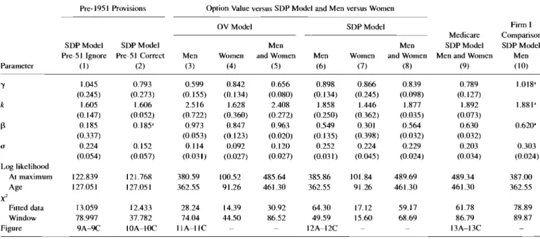
Parameter estimates are shown in table 6.1. The effect of the special plan provisions for the pre-1951 hires is considered first (cols. [ l ] and [2]). Esti- mates for men versus women and stochastic dynamic programming (SDP) ver- sus option value (OV) estimates are then considered (cols. [3]-[8]). Estimates with the “value” of Medicare and firm retiree health insurance benefits counted as equivalent to Social Security benefits, and with firm current employee health insurance benefits counted as equivalent to wage earnings, are also presented (col. [9]). Finally, results imposing firm I parameter estimates (taken from Lumsdaine et al. 1992) on the firm I11 data are reported (col. [lo]).

Pre-1951 Pension Plan Provisions

The estimates in column ( 1 ) are based on the assumption that the pre- 195 1 hires face the same pension plan provisions as later hires. These estimates, as well as those in column (2), are based on a sample of 400 employees. Taken literally, the estimated value of y (1.045) suggests that with respect to retire- ment income employees are essentially risk neutral. The estimated value of k is 1.605, implying that a dollar of retirement benefit income-unaccompanied by work-is valued at 60 percent more than a dollar of income accompanied by work. These estimates are very similar to those obtained in our previous work. The estimated value of

p,

however, is extremely small. If taken literally, it would suggest that in making retirement decisions, future income is given very little weight, compared to income in the current year. Indeed, a value of zero would imply that the decision to retire is based only on the comparison of wage income versus retirement benefits-the replacement ratio-without concern for future possibilities. When the immediate ratio is large enough, the person retires. (Based on our experience elsewhere, we are not inclined to be- lieve this estimate.)

The model fits the data rather well, however, as shown in figures 6.9A and 6.9B. The principal discrepancy between actual and predicted rates occurs at age 5 5 , where the jump in the predicted rates is noticeably less than the jump in the sample rates. The sample data show a 10 percent departure rate at age 5 5 , which is twice as large as the rates shown in the graphs above, based on larger sample sizes. The predicted and actual cumulative departure rates are very close. Based on the likelihood values, the model fits the data better than a model with dummy variables for each age-that is, better than predictions based on average retirement rates by age. The model does not allow directly for an effect of age on retirement.

The primary test of the predictive validity of the model is how well it pre- dicts retirement rates under the 1983 window plan. The model predictions cap- ture the general pattern of retirement under the window, but substantially over- predict retirement rates between ages 55 and 60, as shown in figure 6.9C. The model also predicts some retirements among employees aged 52-54, whereas the actual data show essentially no retirements in this age group.

Table 6.1 Parameter Estimates by Method and Sample

Pre- 195 1 Provisions Option Value versus SDP Modcl and Men versus Women

OV Model SDP Model Firm I

Medicare Comparison

SDP Model SDP Model Men Men SDP Model SDP Model

Pre-5 1 Ignore Pre-5 1 Correct Men Women and Women Men Women and Women Men and Women Men

Parameter ( 1 ) (2) (3) (4) ( 5 ) (6) (7) (8) (9) (10) Y 1.045 (0.245) I .605 (0.147) (0.337) 0.224 (0.054) 0. I 85 0.793 (0.273) I .606 (0.052) 0.185' 0.599 (0.155) 2.516 (0.722) 0.973 (0.053) 0.114 (0.031) 0.842 (0.134) I .62n (0.360) 0.847 (0.123) 0.092 (0.027) 0.656 2.408 (0.272) 0.963 (0.020) 0.120 (0.027) (0.080) 0.898 1.858 (0.134) (0.250) 0.549 (0.135) 0.252 (0.031) 0.866 (0.245) I .446 (0.362) 0.301 0.224 (0.045) (0.398) 0.839 (0.098) 1.877 (0.035) 0.564 (0.032) 0.229 (0.024) 0.789 (0.127) 1.892 (0.073) 0.630 (0.032) 0.203 (0.034) 1.018" k 1.88Ia P 0.620' 0. I52 (0.057) 0.303 (0.024) U Log likelihood At maximum Age X I Fitted data Window Figure 122.839 127.05 1 121.768 127.05 I 380.59 362.55 100.52 91.26 485.64 46 1.30 385.86 362.55 101.84 91.26 489.69 461 3 0 489.34 461.30 387.00 362.55 13.059 78.997 9A-9C 12.433 I OA-l OC 37.782 28.24 74.04 IlA-l1C 14.39 44.50 30.92 86.52 64.30 49.59 12A-I 2C 17.12 15.60 59. I7 68.69 61.78 86.79 I3A-I 3C

Nore: Numbers in parentheses are standard errors. aParameters were fixed at these values.

B al

E

C 50 51 52 53 54 55 56 57 58 59 €0 61 62 63 64 65 Age

1 + Actual Rates + Predicted Rates 1

0 8 0 7 0 6 0 5 0 4 0 3 0 2 0 1 0 50 51 52 53 54 55 56 57 58 59 Bo 61 62 63 64 65 Age

I

-a- Actual Rates + Predicted Rates j

0 9 0 8 0 7 0 8 0 5 0 4 0 3 0 2 0 1 0 50 51 52 53 54 55 56 57 58 58 Bo 61 62 63 64 65 66 Age

1

+ Actual Rates f Predicted Rates 1

Fig. 6.9 Predicted vs. actual (A) annual departure rates, ( B ) cumulative departure rates, and (C) window departure rates: men, ignoring pre-1951 provisions

201 Pension Plan Provisions and Retirement

The estimates in column (2) of table 6.1 are obtained if the special pension plan provisions that pertain to employees hired before 195 1 are used to deter- mine their options. (Because there are so few retirements among employees younger than 55, we have questioned whether these provisions translate into visible alternatives that are actively considered by older employees, or whether in practice these older employees consider their options to be the same as em- ployees of the same age who are covered by the current plan provisions. Thus we have obtained the two sets of estimates.) The estimated parameter values are very similar to those reported in column ( l ) , although to hasten conver- gence the discount factor is set in this case. Predicted versus actual rates are shown in figures 6.1OA-6.1OC. In general, the fit to actual values is close. The major exception is at age 55, and in this case the actual sample rate is abnor- mally high; the predicted rate is more in line with typical retirement rates at this age. The difference in the age-55 retirement rate is reflected in the differ- ence between the actual and predicted cumulative rates through age 60. The model predictions of the effects of the 1983 window are very accurate, with the exception of predictions for employees aged 53-54 and 56-57. The actual sample rates for the 56-57 ages are abnormally low; the typical rates are more like the model predictions. Thus for these ages at least, the model predictions give a more accurate indication of actual behavior than the actual sample values.

Stochastic Dynamic Programming versus “Option Value” Estimates

The two sets of parameter values are shown for men (cols. [3] and [6]), for women (cols. [4] and [7]), and for men and women combined (cols. [5] and [S]). In general, the estimated parameters are similar. The most noticeable dif- ference is that the SDP estimated values of

p

are lower than the OV estimates. For men and women combined, for example, the SDP estimate is 0.564 and the OV estimate is 0.963. The estimated value of k based on the OV model is somewhat larger than the SDP estimate (2.408 vs. 1.877), and the estimated value of y is somewhat smaller (0.656 vs. 0.839).

The OV model fits the sample data considerably better than the SDP model, based on the likelihood and

xz

values pertaining to the fitted data. This is re- vealed graphically for men in figures 6.11A and 6.1 1B versus figures 6.12A and 6.12B. On the other hand, the SDP model predictions of retirement under the 1983 window fit actual retirement rates better than do those of the OV model. This can be seen by comparing figures 6.11 C and 6.12C and in the

x2

values pertaining to the window. Thus, in general, there is no reason to prefer one model over the other.

Separate Estimates f o r Men and Women

The estimates for men and women are not statistically different, judged by likelihood ratio tests. The OV model

x2

statistic is 9.06 (and with four degrees of freedom, the .05 significance level is 9.49), and the SDP model

x2

statistic

0 L 4 4

*

1

50 5 1 52 53 54 5rG <7 5s 59 60 61 62 63 r k k

Age

-~

-

Actual Rates _{_ _} + Predicted Rates .. ~

Fig. 6.10 Predicted vs. actual (A) annual departure rates, ( B ) cumulative departure rates, and (0 window departure rates: men, including pre-1951 provisions

A 0.7 0.6 0.5 0.4 P 0.3 d 0.2 0.1 0 5 0 5 1 5 2 5 3 5 4 5 5 5 6 5 7 5 8 5 9 6 0 6 1 6 2 6 3 6 4 6 5 Age

I + Actual Rates f Predicted Rates I

B 0.9 0.8 0.7 0.6

#

0.5 0.4 0.3 0.2 0.1 0 50 51 52 53 54 55 56 57 58 59 60 61 62 63 64 65 Age

+ Actual Rates + Predicted Rates

c

0.9, I 0 8 0 7 0 6 g 0 5

'

0 4 0 3 0 2 01 0 50 51 52 53 54 55 56 57 58 59 60 61 62 63 €4 65 Age

I+ Actual Rates + Predicted Rates 1

Fig. 6.11 Predicted vs. actual (A) annual departure rates, ( B ) cumulative

0.5-

i l

:

:

:

0.1 50 51 52 53 54 55 56 57 58 59 60 61 62 63 64 65 Age

I + Actua Rates + Predicted Rates

I

0 7 06 0 5 0 4 0 3 0 2 01 0 50 51 52 53 54 55 56 57 58 59 60 61 62 €3 64 65 Age

! + Actual Rates + Predicted Rates I

0 8 0 7 06 0 5 0 4 0 3 0 2 0 1 O J . I , 1 , I I I I , I , I 50 51 52 53 54 55 56 57 58 59 60 61 62 63 64 65 Age

+ Actual Rates + Predicted Rates

Fig. 6.12 Predicted vs. actual (A) annual departure rates, ( B ) cumulative

205 Pension Plan Provisions a n d Retirement

is only 3.98, neither of which is statistically significant. The t-statistics for the individual parameters also suggest that the estimates for men and women are not statistically different. Thus the formal estimates appear to be consistent with the graphical evidence in figures 6.4. 6.5; 6.6, and 6.8 showing that depar- ture rates for men and women are virtually indistinguishable after age 40.

Valuing Medicare

The OV and the SDP models underpredict retirement at age 65 for both men and women. A possible reason for the underprediction is that Medicare insurance becomes available at age 65 and provides an inducement to retire similar to the Social Security inducement. But employees at this firm have health insurance while working, and after retirement the same coverage is pro- vided, at no cost to the retiree. For example, a person who retired at age 60 would be covered by retiree health insurance until age 65. After age 65, medi- cal costs up to the Medicare limit would be paid by Medicare, and any addi- tional costs-that are covered by the firm plan-would be paid by the firm retiree insurance. A simple assumption, albeit one that is unlikely to be pre- cisely true, is that medical insurance is valued at its cost, which is treated by employees as comparable to wage or pension benefit compensation. Following this rule, there are three parts to medical coverage: First, while employed at the firm, health benefits are valued at the cost of insurance to the firm.' Second, if the person retires before age 65, firm pension benefits are increased by the cost of insurance with coverage comparable to the retiree health i n ~ u r a n c e . ~ After age 65, Social Security benefits are increased according to the average payment to persons covered by M e d i ~ a r e . ~ Estimates incorporating these as- sumptions and based on the SDP model for men and women are reported in column (9) of table 6.1.

The parameter estimates are affected very little, relative to comparable esti- mates without these adjustments, shown in column (8). The likelihood value and the fitted-data

x2

statistic are almost the same as in the comparable column (8) estimates, that do not account for the value of medical insurance. In particu- lar, the addition of these measures of the value of medical insurance does noth- ing to explain the departure rate at age 65, as can be seen in figure 6.13A. The

3. This cost was estimated by the average cost at large firms for group insurance with coverage like the plan offered by our fim-$105 and $247 for individual and family coverage, respectively, in 1989 dollars. These costs were deflated to 1982 dollars based on a constructed index of Blue- Cross-Blue-Shield premiums per insured person, obtained from the U.S. Health Insurance Insti- tute (1991). We are grateful to Jonathan Gruber for assistance in developing these numbers.

4. The value of this insurance was estimated by increasing the basic group insurance premium according to age, by 5.4 percent per year for each year after age 50. This rate is based on the annual premium costs by age reported by the Congressional Research Service (1988).

5 . The costs were estimated based on the average 1986 Medicare payments by age to married and single persons, reported in Shoven, Topper, and Wise (chap. I in this volume). The 1986 values were deflated to 1982 dollars based on the Blue-Cross-Blue-Shield index described in n. 3, above. Linear Interpolation was used to convert the payments by age interval, reported by Sho- ven, Topper, and Wise, to payments for each age.

0.4 2 d 0.3 0.2 0.1 0 50 51 52 53 54 55 56 57 56 59 W 61 62 63 64 65 Age

I + ~ c t u a l Rates + Predicted Rates I

B

50 51 52 53 54 55 56 57 58 59 W 61 62 83 64 65

m e

1 + Actual Rates -I- Predicted Rates

I

c

0.91 I 0.6 0.7 0,6 0.5

’

0.4 0.3 0.2 0.1 0 50 51 52 53 54 55 56 57 56 59 W 61 82 63 64 65 Age I f Actual Rates + 1-P

Fig. 6.13 Predicted vs. actual (A) annual departure rates, ( B ) cumulative

departure rates, and (C) window departure rates: men and women, SDP,

207 Pension Plan Provisions and Retirement

actual rate is .636, but the predicted rate is only .215, somewhat lower than the predicted rate without accounting for medical insurance (.277, based on col. [8] estimates). In addition, the model yields worse predictions of retirement under the window plan, judging by the window

x2

statistic. Thus these results lend no support to the conjecture that retirement at age 65 is strongly affected by the availability of Medicare at that age. However, these exploratory results should not be interpreted to mean that Medicare does not matter. It may well be that the rough specification that we experimented with does not capture the effect of Medicare but that a more careful treatment of the value of medical coverage would show an effect. For example, the assumption that medical in- surance is valued at its cost may be incorrect.

Estimates from Firms I and I l l Compared

The parameter estimates based on firm I11 data are surprisingly close to those based on firm I data. Results, for firm 111, with parameter estimates set to those that we obtained for firm I (Lumsdaine et al. 1992) are shown in col- umn (10) of table 6.1 .6 By comparing the estimates in columns (6) and (lo), it can be seen that the firm I estimates for men are very close to the estimates for firm 111, based on the SDP specification. The hypothesis that the parameters are the same cannot be rejected, based on a likelihood ratio test. From the

x2

statistics, however, it is clear that the firm I parameter estimates do not fit the data or predict departure rates under the window plan quite as well as the firm 111 estimates. Option value model estimates for the two firms (not shown) are also similar but not as close as the SDP estimates, and the hypothesis that the estimates are the same is rejected at the 5 percent level. Again, based on

x2

statistics, the firm I estimates do not fit the data or predict window departure rates as well as the firm 111 parameter estimates. On balance, however, the results provide strong confirmation that employees in these two firms react similarly to the incentives inherent in pension plan provisions.

6.4 Summary and Conclusions

The data for firm 111 confirm a principal conclusion based on firm I data. It is clear that the changes in retirement rates by age correspond closely to provis- ions of the pension plan. And, as for the results based on firm I, we find that the OV and the SDP models yield similar results. There is no apparent reason to choose one over the other, except based on numerical simplicity. In this case, the OV model fits the sample data better than the SDP model, but the SDP model predicts the window plan retirement rates better than the OV model. We also find that there is essentially no difference between the retirement behavior of men and women. There is some indication that women may be slightly more

6. The scale parameter u was estimated; this normalization enables comparison of the results from the two firms.

likely than men to take early retirement between ages 55 and 60. But at most ages, the annual retirement rates of men and women are very close. In addition, we explored the possibility that retirement at age 65 is induced by Medicare benefits that become available at that age. Our method of incorporating medi- cal insurance, however, did little to explain the large retirement rates at age 65. Thus we are still left with an “age-65 retirement effect” that is not explained by monetary gain.

Appendix

The “option value” and stochastic dynamic programming models used in the analysis are described.

The Option Value Model

function G,(r) can be decomposed into two components, ( A l l

where g,(r) and +,(r) distinguish the terms in G,(r) containing the random ef- fects, w and

t,

from the other terms. If whether the person is alive in future years is statistically independent of his earnings stream and of the individual effects w, and

&,

g,(r) and +,(r) are given by

( A 2 4 g,(r) = ~:I,’PS-‘.rr(slW,(Y?)

+

~ ~ _ , P ” . r r ( s l t ) [ ~ , ( ~ ~ ~ ( ~ ) ) y l -

Given the specification as described via equations (1)-(5) in the text, the

G,(r) = g,(r)

+

+,(d

1

CS=,

P”-Wslt) [E,(kB,(f))Yl 3

+,(r) = C:Ir’P~-~.rr(slt)E,(o. -

tJ

(A2b)

where .rr(sIt) denotes the probability that the person will be alive in year s,

given that he is alive in year t. Given the random Markov assumption, +,(I) can

be written as

(‘43) +,(r) = C:I:PS-r.rr(slt)p”-‘(w,

-

6,)

= K ,( r) u ,,

where K,(r) = E,:=:(Pp)”-‘.rr(slt) and u, = w, -

5,.

The simplification results from the fact that at time t the expected value of u,, = o , ~ -

6,

is p‘-’v,, for all future years s. (The term K,(r) cumulates the deflators that yield the present value in year t of the future expected values of the random components of utility. The further r is in the future, the larger is K,(r). That is, the more distant the potential retirement age, the greater the uncertainty about it, yielding a heteroskedastic disturbance term.) Thus, G,(r) may be written simply as

209 Pension Plan Provisions and Retirement

('44)

If the employee is to retire in year

r,

G , ( r ) must be less than zero for every potential retirement age r in the future. If r: is the r that yields the maximum value of g,( r)/K,(r), the probability of retirement becomes

( - 4 5 ) Pr[Retire in year

r]

= Pr[g,(r;)/K,(r;)

<

-wJ

.

If retirement in only one year is considered, this expression is all that is needed. More generally, retirement decisions may be considered over two or more consecutive years. In this case, the retirement probabilities are simply an exten- sion of equation (10). The probability that a person who is employed at age t will retire at age T

>

r

is given by

('46)

G,(r) = g,(r)

+

K,(r)u,.

Pr[R =

TI

= Pr[g,(r;)/K,(r:)

>

-u,,

. .

. , g ~ - l ( r ~ - , ) / K ~ - l ( r ~ - , )

>

g7(r:YK7(r;)

<

-uJ

.

The probability that the person does not retire during the period of the data is given by

('47) Pr[R

>

r ] = Pr[g,(r;)/K,(r:)

>

-ur,

. . .

, g r - , ( r ; - , ) / K r - i ( r ~ - i )

>

-u,-i, gr(r;)/Kr(r;)

>

- ~ r l

.

This is a multinomial discrete choice probability with dependent error terms u,.

Finally, we assume that us follows a Gaussian Markov process, with (A81

where the initial value, u,, is i.i.d. N(0,a2) and is independent of E,. The covari- ance between u, and u,,, is pVar(u,), and the variance of u,, for T

>

r,

is

The estimates in this paper are based on retirement decisions in only one year, and the random terms in equation ( 5 ) are assumed to follow a random walk, with p = 1. In this case, the covariance between u, and uT+, is Var(u,), and the variance of u,, for T 5

r,

is uz

+

(T - t)cr;. Prior estimates show that one- and multiple-year estimates are very similar. (Estimates based on several consecutive years and with p estimated are shown in Stock and Wise 1990b. These generalizations have little effect on the estimates.)

u , ~ = pu,-,

+

E , , with E , i.i.d. N ( 0 , a:),

(p*lT-/))cr?

+

( Z , y

pqa;.

The Stochastic Dynamic Programming Model

The dynamic programming model is based on the recursive representation of the value function. At the beginning of year

r,

the individual has two choices: retire now and derive utility from future retirement benefits, or work for the year and derive utility from income while working during the year and re- taining the option to choose the best of retirement or work in the next year. Thus the value function W, at time

r

is defined as

W, = max{E,[U,(Y,)

+ E , , +

PW,+,I,

E,[C.~=,P"(U,(B,(~))

+ E ~ J I I , with W,+, = max{E,+,[~,(Y,+,)

+

%+, + PW,+21,

E,+,[C:=,+, P'-'-'(U,(B,(r

+

1)) + E*T)119

(A91

etc., where

P

is the discount factor and, as in the option value model, S is the year beyond which the person will not live.

Because the errors E ! , are assumed to be i.i.d., E,E,,,, = 0, for T

>

0. In

addition, in computing expected values, each future utility must be discounted by the probability of realizing it, i.e., by the probability of surviving to year T

given that the worker is alive in year t, r ( T 1 t ) . With these considerations, the

expression (A9) can be written as

W, = max{W,,

+

E , , ,

Wzf

+

E ~ , } , where

W , ,

= U,(Y,)

+

P.rr(f

+

1

I

f ) E , W,+, and

The worker chooses to retire in year f if

W , ,

+

E , ,

<

W2,

+

E ~ , ; otherwise he

continues working. The probability that the individual retires is P r [ W , ,

+

E , ,

<

W2,

+

E J . If a person works until the mandatory retirement age (741, he

retires and receives expected utility W2,,,. Recursions and Computation

With a suitable assumption on the distribution of the errors E,,, the expres-

sion (A10) provides the basis for a computable recursion for the nonstochastic terms

m,,

in the value function. The extreme value and normal distribution versions of the model are considered in turn.

Extreme value errors. Following Berkovec and Stern (1988), the E , , are as-

sumed to be i.i.d. draws from an extreme value distribution with scale parame- ter u. Then, for the years preceding mandatory retirement, these assumptions together with equation (16) imply that

E,W,+,/u

=

Fl+l

= ye

+

1n[exp(w,,+,/u)

+

~ ~ p ~ ~ z l + l ~ ~ ~ ~

= ye

+

ln[exp(Uw(Y,+,)/u)exp(P.rr(t

+

2 It

+

1)pI+J

+

e x ~ ( W ~ , + ~ / u ) I , where y, is Euler's constant. Thus equation (A1 1 ) can be solved by backward recursion, with the terminal value coming from the terminal condition that The extreme value distributional assumption provides a closed form expres- ( A l l )

-

F,,, - WZ,,,.

sion for the probability of retirement in year t:

(A12) Pr[Retire in year t] = Pr[W,,

+

_<

_{W Z f}

+

E J

211 Pension Plan Provisions and Retirement

Gaussian errors. Following Daula and Moffitt (1989), the E , , are assumed to be independent draws from an N(0,u2) distribution. The Gaussian assumption provides a simple expression for the probability of retiring:

(A 13) Pr[Retire in year t ]

= Pr[(EI,

-

EJ@

<

(W2,

-

W,,)/-\IZa]

= @(a,), where a, =

(W2,

-

wlr)/@.

Then the recursion (A10) becomes (A 14) E , W l + , I ~

=

k + I

= ( w l r + l m l

-

@(Q,+I)l

+

(%lA,wwl+,)

+ .i2$(.,+,)

where +(*) denotes the standard normal density and @(*) denotes the cumula- tive normal distribution function. As in equation (A13), @(a,> is the probability that the person retires in year r and receives utility

w21,

plus utility from E(E>,

I

E , , - E * ,

<

w2,

-

WIJ.

The latter term, plus a comparable term when the person continues to work, yields the last term in equation (A14).

Individual-specific Effects

Individual-specific terms are modeled as random effects but are assumed to be fixed over time for a given individual. They enter the two versions of the dynamic programming models in different ways. Each is discussed in turn.

Extreme value errors. Single-year utilities are

(A15a) Uw(Yr) =

Yi

1

(A15b) U,(B,(s)) = [qk4(s)l7 9

where q k is constant over time for the same person, but random across individ- uals. Specifically, it is assumed that q is a lognormal random variable with mean one and scale parameter A: q = exp(Az

+

1/2 A2), where

z

is i.i.d. N(0,l). A larger A implies greater variability among employee tastes for retirement versus work; when A = 0 there is no variation and all employees have the same taste.

Normal errors. In this case, the unobserved individual components are as- sumed to enter additively, with

(A16a) (A 16b)

UJY,) = y:

+

L

U,(B,(s)) = [kB,(s)lY t

where y and k are nonrandom parameters, as above, but

5

is a random additive taste for work, assumed to distributed N(0,A2). When h = 0, there is no taste variation.

In summary, the dynamic programming models are given by the general recursion equation (A9). It is implemented as shown in equation (A1 1) under

the assumption that the c,, are i.i.d. extreme value, and as shown in equation

(A14) under the assumption that e!, are i.i.d. normal. T h e retirement probabili- ties are computed according to equations (A12) and (A13) respectively. T h e fixed effect:, specifications are given by equations (A15) and (A16). T h e un- known parameters to be estimated are y. k,

p,

u, and A. Because of the different distributional assumptions, the s c d e parameter cr is not comparable across option value or dynamic progratnrning models, and h is not comparable across the two dynatnic progranznzing models.

References

Ausink, John A. 1991. The effect of changes in compensation on a pilot’s decision to Berkovec, James, and Steven Stem. 199 I . Job exit behavior of older men. Ecoriometrica

Bulow, J. 1981. Early retirement pension benefits. NBER Working Paper no. 654. Cam- bridge, Mass.: National Bureau of Economic Research.

Congressional Research Service. 1988. Costs and effects of extending health insurance coverage. Washington, D.C.: Library of Congress.

Dada, Thomas V., and Robert A. Moffitt. 1991. Estimating a dynamic programming model of army reenlistment behavior. In Militup compensation andpersonnel refen-

tion; Models and evidence, ed. C. L. Gilray, D. K. Horne, and D. Alton Smith. Alex-

andria, Va.: U.S. Army Research Institute for the Behavioral and Social Sciences. Kotlikoff, Laurence J., and David A. Wise. 1985. Labor compensation and the structure

of private pension plans: Evidence for contractual versus spot labor markets. In Pen-

sions, labor; and individual choice, ed. D. Wise, 55-85. Chicago: University of Chi-

cago Press.

. 1987. The incentive effects of private pension plans. In Issues in pension eco-

nomics, ed. Z. Bodie, J. Shoven, and D. Wise. 283-339. Chicago: University of Chi-

cago Press.

. 1988. Pension backloading. wage taxes, and work disincentives. In Tax policy

and the economy, vol. 2, ed. L. Summers, 161-96. Cambridge: MIT Press.

Lazear, Edward P. 1983. Pensions as severance pay. In Financial aspects ofrhe United

Srates pension system, ed. Z . Bodie and J. Shoven, 57-85. Chicago: University of

Chicago Press.

Lumsdaine, Robin L., James H. Stock, and David A. Wise. 1990. Efficient windows and labor force reduction. Journul of Public Economics 43: 13 1-59.

. 1991. Windows and retirement. Annales d’Economie et de Statistique 20/

. 1992. Three models of retirement: Computational complexity versus pre- dictive validity. In Topics in fhe economics o f a g i n g , ed. D. Wise, 19-57. Chicago: University of Chicago Press.

Stock, James H., and David A. Wise. 1990a. Pensions, the option value of work, and retirement. Economefrica 58, no. 5 (September): 1151-80.

.

1990b. The pension inducement to retire: An option value analysis. In Issues in

the economics ofuging, ed. D. Wise, 205-24. Chicago: University of Chicago Press. U S . Health Insurance Institute. 1991. Sourcebook ofhealth insurance data, 1990. New

York: U.S. Health Insurance Institute.

leave the air force. Ph.D. dissertation, Harvard University. 59( 1 ): 189-2 10.