TECHNICAL UNIVERSITY OF CLUJ-NAPOCA
ACTA TECHNICA NAPOCENSIS
Series: Applied Mathematics, Mechanics, and Engineering Vol. 60, Issue III, September, 2017
STUDY OF CHANGING GEOMETRIC CHARACTERISTICS IN
PROXIMAL FEMORAL BONE AFFECTED BY OSTEOPOROSIS IN
COMPLIANCE WITH SINGH INDEX
Adrian Ioan BOTEAN
Abstract: The present study aims to analyze the geometric characteristics of four cross - sections (femoral head, femoral neck, intertrochanteric and diaphysis) from the proximal femoral bone area. Depending on the process of degradation of trabecular tissue generated by osteoporosis, a process characterized by the Singh index, the geometric characteristics of the cross – section were determined in different areas of the proximal femoral bone: area of shape, the coordinates of the center of gravity, moment of inertia, product of inertia, radius of gyration and static moments of surface.
Key words: proximal femoral bone, osteoporosis, trabecular tissue, cortical tissue, geometrical
characteristics of cross section
1. INTRODUCTION
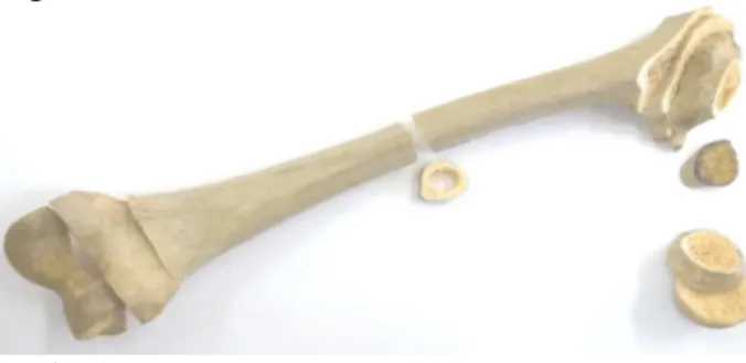
The present study aims to analyze the geometric characteristics of four cross - sections (femoral head - FH, femoral neck - FN, intertrochanteric - IT and diaphysis - D) from the proximal femoral bone (PFB) area, according to Figure 1.
Fig. 1. Femoral bone sectioned in the cross - section plane.
In the computational relations of stresses and deformations produced by axial loading (produced by the axial forces, N) or the shear loading (produced by the cutting forces, T), the cross – section (CS) of the proximal femoral bone (Fig.2), affected by osteoporosis (OP), occurs in its simplest form, namely by the value of its area of shape (AOS). For this cases of loading the CS geometry does not play any role.
Fig. 2. The structure of PFB. a) longitudinal section; b) sagittal section.
In the study of the state of stresses and deformations caused by other simple loading, such as bending, torsion, or in the case of composite loading, geometric notions of a more complex form than the CS area occur. These are moments of varying degrees of CS, such as static moments of surface (SMOS) (moments of the first degree), moment of inertia (MOI) and polar moment of inertia (PMOI), product of inertia (POI), radius of gyration (ROG), section modulus (axial – SMA and polar SMP). Their values depend on both size and the shape of the CS studied.
dimensions (outer distance, inner distance), FN dimensions (outer distance, inner distance), FH dimensions (outer distance, inner distance), IT distance. All these dimensions are determined mainly by anteroposterior (AP) X-rays or scanning by computer tomography (CT) [1, 2, 3, 4, 5, 6, 7] but also with digital photography [8]. If reference is made to the geometric characteristics of the CS (AOS, SMOS, MOI, PMOI, POI, ROG, SMA, SMP) can be shown that the number of scientific works which meet the subject is relatively low [9, 10].
In order to determine the size of these parameters, it is necessary to know in depth the architectural microstructure of the trabecular tissue [11, 12, 13, 14, 15]. If the trabecular structure is affected by osteoporosis, using the Singh index and bone mineral density (BMD), its degradation may be highlighted [16, 17, 18].
It is assumed that the trabecular dimensions of the different trajectory groups (primary and secondary compression group, main and secondary stretch group) depend on the magnitude of the mechanical stress level of the human body and that when the BMD decreases trabecular pattern register a regression, in a predictable sequence. In 1970 M. Singh, A.R. Nagrath and P.S. Maini proposed a classification system based on this phenomenon by a comparative x-ray of the PFB radiograph showing OP with radiographies considered to be „normal”. This classification system is called Singh’s system. Under this system there are six degrees of visibility of the trabecular structure of the PFB, according to Figure 3. Grades 6 to 4 are considered normal and grades 3 to 1 indicate OP.
Fig. 3. Hierarchy of the Singh index.
Currently, BMD is the surrogate parameter of bone mass in OP. Osteodensitometry is the non-invasive method
that allows BMD measurement, and as long as the identification of the OP remains tributary to the quantitative element, it is the main method of diagnosing the disease in the preclinical stage, that is before the occurrence of the fractures. From the perspective of the OP’s particularities regarding the architecture of the trabecular structure of the PFB and the fact that it is affected by a gradual regression, the geometric characteristics of the four CS mentioned above (Fig.2) were determined.
2. METHODS
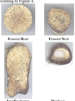
The femoral bone chosen for the study is estimated to be characteristic of an overweight person with a body mass index BMI=25.6. Following sectioning in the transverse plane of the PFB (Fig.1), the following four CS were taken into consideration: FH, FN, IT and D, according to Figure 4.
Femoral Head Femoral Neck
InterTrochanter Diaphysis
Fig. 4.Cross Sections considered.
dimensions are 1,584x1,696 pixels and the horizontal and vertical resolution is 1,200 dpi, in the CS of the IT area the dimensions are 2,208x4,000 pixels and the horizontal and vertical resolution is 1,200 dpi, in the case of the CS of the D area the dimensions are 1,648x1,584 pixels and the horizontal and vertical resolution is 1,200 dpi. The next step is to highlight the structure of the cortical and trabecular tissue in the plane of interest by eliminating in-depth planes using an image editing software, as shown in Figure 5.
Fig. 5. Define the current plane for the CS of the FN.
The CS in the final form is shown in Figure 6.
Fig. 6. The CS, in the final form, of the FN.
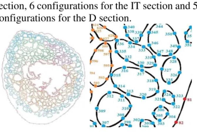
In the next step, the current surface is discretized through a number of nodes, according to Figure 7. For the FH section were needed 5,791 nodes, for the FN section were needed 3,500 nodes, for the IT section were needed 10,117 nodes, for the D section were needed 855 nodes, in total 20,263 nodes.
By scaling the image using Digimizer software, the position can be determined in the cartesian coordinate of each node.
Starting from such a configuration, considered to be the basic section, by introducing the cartesian coordinates in the AutoCad software, also taking into account the Singh index of degradation of the trabecular structure is obtained, according to Figure 8, Figure 9, Figure 10, Figure 11, 5 configurations for the FH section, 6 configurations for the FN
section, 6 configurations for the IT section and 5 configurations for the D section.
Fig. 7. Numbering nodes.
According to Figure 8, the CS of the FH considered healthy has a number of 904 traves. When the trabecular structure is affected by OP, for Grade 4 there are 690 traves with a deterioration percentage of 23.67 relative to the structure considered to be healthy; for Grade 3 there are 424 traves with a deterioration percentage of 53.09 compared to the structure considered to be healthy; for Grade 2 there are 114 traves with a deterioration percentage of 87.38 compared to the structure considered to be healthy and Grade 1 there are 27 traves with a 97.01 damage percentage compared to the structure considered to be healthy.
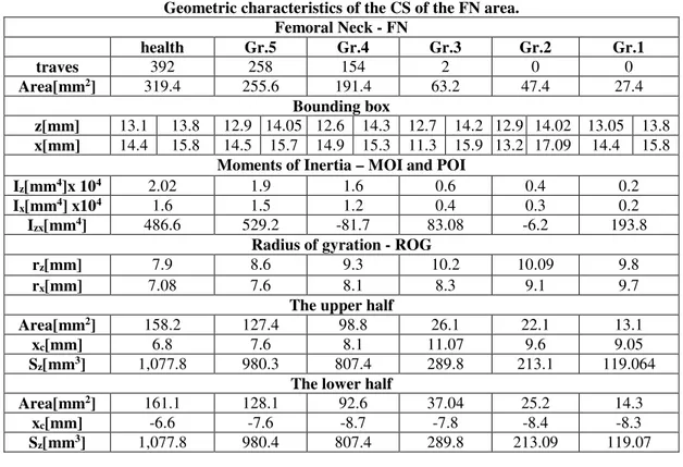
According to Figure 9, the CS of the FN considered healthy has a number of 392 traves. When the trabecular structure is affected by OP, for Grade 5 there are 258 traves with a deterioration percentage of 34.18 relative to the structure considered to be healthy; for Grade 4 there are 154 traves with a deterioration percentage of 60.71 compared to the structure considered to be healthy; for Grade 3 there are 2 traves with a deterioration percentage of 99.48 compared to the structure considered to be healthy; for Grade 2 and 1 there is no longer a travee recorded with a deterioration percentage of 100 compared to the structure considered to be healthy.
256 traves with a deterioration percentage of 85.04 compared to the structure considered to be healthy; for Grade 2 there are 81 traves with a 95.26 damage percentage compared to the structure considered to be healthy and Grade 1 there are 20 traves with a 98.83 damage percentage compared to the structure considered to be healthy.
healthy Grade 4 Grade 3
Grade 2 Grade 1
Fig. 8. The CS of the FH area.
healthy Grade 5 Grade 4
Grade 3 Grade 2 Grade 1
Fig. 9. The CS of the FN area.
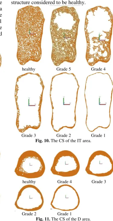
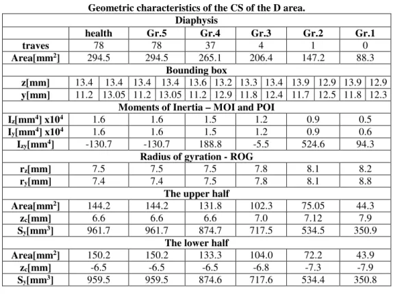
According to Figure 11, the CS of the D considered healthy has a number of 78 traves. When the trabecular structure is affected by OP, for Grade 4 there are 37 traves with a deterioration percentage of 52.56 relative to the structure considered to be healthy; for Grade 3 there are 4 traves with a deterioration percentage of 94.87 compared to the structure considered to be healthy; for Grade 2 there are 1 trave with a deterioration percentage of 98.71 compared to the structure considered to be healthy and Grade 1 there is no longer a travee recorded with a
deterioration percentage of 100 compared to the structure considered to be healthy.
healthy Grade 5 Grade 4
Grade 3 Grade 2 Grade 1
Fig. 10. The CS of the IT area.
healthy Grade 4 Grade 3
Grade 2 Grade 1
Fig. 11. The CS of the D area.
Analytically, it is admitted that the surface area A is composed of a number of surface elements with infinitely small size, of area dA. Is defined the SMOS (or moment of the first degree of surface) in relation to the axes Oz and Oy the sum of the products between the infinite small areas dA of the surface elements and the distances of these elements at thw considered axis [19]. SMOS are measured in mm3, cm3 etc.
The coordinates of the center of gravity of the complex surface can be determined by the following relationship:
= = ∙ + ∙+ + ⋯ ++ ⋯ + ∙ (2)
= == ∙ + ∙+ + ⋯ ++ ⋯ + ∙ (3)
MOI and POI can be determined through Steiner’s formulas:
(
)
∑ +
=
=
n
1
i i
2 C z
z I y A
I
i
i =∑
(
+)
=
n
1
i i
2 C y
y I z A
I
i i
(4)
(
)
∑ +
=
=
n
1
i zy C C i
zy I y z A
I
i i i i
(5)
3. RESULTS
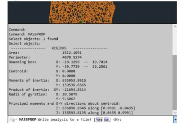
Once the geometries of the analyzed models are defined in the AutoCAD software, the MASSPROP command (according to Figure 12) generates the values for the following characteristics of the CS: moment of inertia (MOI) and polar moment of inertia (PMOI),
product of inertia (POI), radius of gyration (ROG), etc.
Fig. 12. The geometric characteristics generated in AutoCAD with the MASSPROP command.
Thus, in Table 1 the geometric characteristics of the CS of the FH area are centralized; in Table 2 the geometric characteristics of the CS of the FN area are centralized; in Table 3 the geometric characteristics of the CS of the IT area are centralized and in Table 4 the geometric characteristics of the CS of the D area are centralized.
Table 1 Geometric characteristics of the CS of the FH area.
Femoral Head - FH
health Gr.5 Gr.4 Gr.3 Gr.2 Gr.1
traves 904 904 690 424 114 27
Area[mm2] 821.5 821.5 697.7 492.3 164.4 82.6
Bounding box
z[mm] 20.8 20.9 20.8 20.9 20.7 21.0 20.6 21.1 21.6 20.1 20.6 21.1
x[mm] 21.3 21.4 21.3 21.4 21.3 21.4 21.1 21.6 21.2 21.5 20.5 22.2
Moments of Inertia – MOI and POI
Iz[mm4] x104 9.4 9.4 8.4 7.7 3.3 1.8
Ix[mm4] x104 9.01 9.01 8.06 7.3 3.2 1.6
Izx[mm4] -2,479.6 -2,479.6 -829.7 -876.5 -874.03 -492.5
Radius of gyration - ROG
rz[mm] 10.7 10.7 11.0 12.5 14.3 15.09
rx[mm] 10.4 10.4 10.7 12.2 14.1 14.2
The upper half
Area[mm2] 407.9 407.9 345.7 241.7 82.4 39.6
xc[mm] 9.1 9.1 9.4 11.3 12.8 14.2
Sz[mm3] 3,737.3 3,737.3 3,252.7 2,745.7 1,060.5 566.2
The lower half
Area[mm2] 413.6 413.6 351.9 250.6 82.06 43.0
xc[mm] -9.03 -9.03 -9.2 -10.9 -12.9 -13.1
Table 2 Geometric characteristics of the CS of the FN area.
Femoral Neck - FN
health Gr.5 Gr.4 Gr.3 Gr.2 Gr.1
traves 392 258 154 2 0 0
Area[mm2] 319.4 255.6 191.4 63.2 47.4 27.4
Bounding box
z[mm] 13.1 13.8 12.9 14.05 12.6 14.3 12.7 14.2 12.9 14.02 13.05 13.8
x[mm] 14.4 15.8 14.5 15.7 14.9 15.3 11.3 15.9 13.2 17.09 14.4 15.8
Moments of Inertia – MOI and POI
Iz[mm4]x 104 2.02 1.9 1.6 0.6 0.4 0.2
Ix[mm4] x104 1.6 1.5 1.2 0.4 0.3 0.2
Izx[mm4] 486.6 529.2 -81.7 83.08 -6.2 193.8 Radius of gyration - ROG
rz[mm] 7.9 8.6 9.3 10.2 10.09 9.8
rx[mm] 7.08 7.6 8.1 8.3 9.1 9.7
The upper half
Area[mm2] 158.2 127.4 98.8 26.1 22.1 13.1
xc[mm] 6.8 7.6 8.1 11.07 9.6 9.05
Sz[mm3] 1,077.8 980.3 807.4 289.8 213.1 119.064 The lower half
Area[mm2] 161.1 128.1 92.6 37.04 25.2 14.3
xc[mm] -6.6 -7.6 -8.7 -7.8 -8.4 -8.3
Sz[mm3] 1,077.8 980.4 807.4 289.8 213.09 119.07
Table 3 Geometric characteristics of the CS of the IT area.
InterTrochanteric - IT
health Gr.5 Gr.4 Gr.3 Gr.2 Gr.1
traves 1,712 1,229 591 256 81 20
Area[mm2] 1,512.1 1,208.2 746.05 388.8 227.7 147.1 Bounding box
z[mm] 18.3 19.7 18.2 19.7 18.9 19.07 18.0 20.02 17.6 20.3 19.2 18.7
x[mm] 39.7 36.2 35.7 40.2 32.6 43.4 34.2 41.7 35.05 40.9 34.9 41.04
Moments of Inertia – MOI and POI
Iz[mm4] x104 63.5 51.7 34.5 22.2 14.3 8.7
Ix[mm4] x104 13.9 12.6 9.3 6.7 4.2 2.8
Izx[mm4] -21,654.8 -21,892.8 -15,124.5 -8,020.3 -4,965.4 -3,655.9 Radius of gyration - ROG
rz[mm] 20.5 20.6 21.5 23.9 25.1 24.4
rx[mm] 9.6 10.2 11.1 13.1 13.5 13.8
The upper half
Area[mm2] 781.3 579.2 321.1 185.7 109.02 71.4
xc[mm] 17.1 18.2 20.9 22.06 23.3 22.1
Sz[mm3] 13,411.5 10,559.2 6,712.5 4,098.6 2,546.1 1,585.08 The lower half
Area[mm2] 730.8 628.9 424.8 203.1 118.7 75.6
xc[mm] -18.3 -16.7 -15.7 -20.1 -21.4 -20.9
Table 4 Geometric characteristics of the CS of the D area.
Diaphysis
health Gr.5 Gr.4 Gr.3 Gr.2 Gr.1
traves 78 78 37 4 1 0
Area[mm2] 294.5 294.5 265.1 206.4 147.2 88.3 Bounding box
z[mm] 13.4 13.4 13.4 13.4 13.6 13.2 13.3 13.4 13.9 12.9 13.9 12.9
y[mm] 11.2 13.05 11.2 13.05 11.2 12.9 11.8 12.4 11.7 12.5 11.8 12.3
Moments of Inertia – MOI and POI
Iz[mm4] x104 1.6 1.6 1.5 1.2 0.9 0.5
Iy[mm4] x104 1.6 1.6 1.5 1.2 0.9 0.6
Izy[mm4] -130.7 -130.7 188.8 -5.5 524.6 94.3 Radius of gyration - ROG
rz[mm] 7.5 7.5 7.5 7.8 8.1 8.2
ry[mm] 7.4 7.4 7.5 7.8 8.1 8.8
The upper half
Area[mm2] 144.2 144.2 131.8 102.3 75.05 44.3
zc[mm] 6.6 6.6 6.6 7.0 7.12 7.9
Sy[mm3] 961.7 961.7 874.7 717.5 534.5 350.9 The lower half
Area[mm2] 150.2 150.2 133.3 104.0 72.2 43.9
zc[mm] -6.5 -6.5 -6.5 -6.8 -7.3 -7.9
Sy[mm3] 959.5 959.5 874.6 717.6 534.4 350.8
4. CONCLUSIONS
Depending on the process of degradation of the trabecular tissue generated by osteoporosis, a process characterized by the Singh index, the geometric characteristics of the cross - section were determined in different areas of the proximal femoral bone: area of shape, the coordinates of the center of gravity, moment of inertia, product of inertia, radius of gyration and static moments of surface.
These geometric characteristics of cross – section play an important role in determining the stress and deformation state as well as the buckling stability of the proximal femoral bone. From the results it can be pointed out that the area of shape, moment of inertia, product of inertia and static moments of surface registers a progressive regression with the evolution of osteoporosis, this signifying a weakening of the resistance in the proximal femoral bone area.
5. ACKNOWLEDGEMENTS
This study was made possible by the technical support given by Curean Rareş, Duma Irina and Filipovici Dumitreasa Emil, students at the Automotive Engineering and
Transportations Department, Faculty of Mechanics, Technical University of Cluj Napoca, Romania.
6. REFERENCES
[1] Moulton D.L., Lindsey R.W., Gugala Z.,
Proximal femur size and geometry in
cementless total hip arthroplasty patients,
F1000 Research 2015, 4:161.
[2] Patton M.S., Duthie R.A., Sutherland A.G.,
Proximal femoral geometry and hip
fractures, Acta Orthop. Belg., 2006, 72,
51-54.
[3] Robin J., Kerr Graham H., Selber P., Dobson F., Smith K., Baker R., Proximal femoral
geometry in cerebral palsy. A population –
based cross – sectional study, The Journal of
bone & joint surgery (Br), 2008; 90-B: 1372-1379.
[4] Panula J., Savela M., Jaatinen P.T., Aarnio P., Kivela S.L., The impact of proximal femur
geometry on fracture type – a comparison between cervical and trochanteric fractures
with two parameters, Scandinavian Journal
of Surgery, 97: 266-271, 2008.
[5] Imren Y., Sofu H., Dedeoglu S.S., Desteli E.E., Cabuk H., Kir M.C., Predictive value of
femoral geometry for hip fracture in the elderly: what is the role of the true moment arm?, Arch. Med. Sci. Civil Dis., 2016; 1: s58 – e62.
[6] Pocock N.A., Noakes K.A., Majerovic Y., Griffiths M.R., Magnification error of
femoral geometry using fan beam
densitometers, Calcif. Tissue Int., 1997, 60:
8-10.
[7] Nissen N., Hauge E.M., Abrahamsen B., Jensen J.E.B., Mosekilde L., Brixen K.,
Geometry of the proximal femur in relation to
age and sex: a cross – secţional study in
healthy adult danes, Acta Radiol., 2005;
46:514-518.
[8] Unnanuntana A., Toogood P., Hart D., Cooperman D., Grant R.E., Evaluation of
proximal femoral geometry using digital
photographs, Journal of Orthopedic
Research, 2010, 28:1399-1404.
[9] Hui L., Kang L., Taehyong K., Aidong Z., Murali R., Spatial modeling of bone
microarchitecture, Proc. SPIE 8290, 82900P,
2012.
[10] Yang L., Burton A.C., Bradburg M., Nielson C.M., Orwoll E.S., Eastell R.,
Distribution of bone density in the proximal femur and its association with hip fracture
risk in older men: the MrOS Study, J Bone
Miner Res. 2012; 27(11): 2314-2324.
[11] Wehrli F.W., Role of Cortical and
Trabecular Bone Architecture in
Osteoporosis, cds.ismrm.org.
[12] Boutroy S., Vilayphiou N., Roux J.P., Delmas P.D., Blain H., Chapurlat R.D., Chavassieux P., Comparison of 2D and 3D
bone microarchitecture evaluation at the
femoral neck, among postmenopausal women
with hip fracture or hip osteoarthritis, Bone,
2011; 49:1055-1061.
[13] Blain H., Chavassieux P., Portero-Muzy N., Bonnel F., Canovas F., Chammas M., Maury P., Delmas P.D., Cortical and trabecular
bone distribution in the femoral neck in
osteoporosis and osteoarthritis, Bone, 2008;
43:862-868.
[14] Chen H., Zhou X., Fujita H., Onozuka M., Kubo K.Y., Age-Related Changes in
Trabecular and Cortical Bone
Microstructure, Int. J. of Endocrinology,
vol.2013, ID 213234.
[15] Brandi M.L., Microarchitecture, the key to
bone quality, Rheumatology, 2009;
48:iv3-iv8.
[16] Singh M., Nagrath A.R., Maini P.S.,
Changes in trabecular pattern of the upper
end of the femur as an index of osteoporosis,
The Journal of Bone & Joint Surgery, 1970; 52A:457-467.
[17] Vaseenon T., Luevitoonvechkij S., Namwongphrom S., Rojanasthien S.,
Proximal femoral bone geometry in
osteoporotic hip fractures in Thailand, J.
Med. Assoc. Thai, 2015: 98 (1): 77-81. [18] Thomas C.D.L., Mayhew P.M., Power J.,
Poole K.E.S., Loveridge N., Clement J.G., Burgoyne C.J., Reeve J., Femoral Neck
Trabecular Bone: Loss With Aging and Role
in Preventing Fracture, J Bone Miner Res.
2009; 24(11): 1808-1818.
[19] Botean A.I., Rezistenţa materialelor.
Solicitări simple, U.T.PRESS, Cluj-Napoca,
2017
Studiul modificării caracteristicilor geometrice ȋn osul femural proximal afectat de osteoporoză,
ȋn concordanţă cu indicele Singh
Rezumat: Prezentul studiu ȋşi propune analiza caracteristicilor geometrice a patru secţiuni transversale (cap femural, col femural, intertrohanteric şi diafiză) din zona osului femural proximal. În funcţie de procesul de degradare a ţesutului trabecular generat de către osteoporoză, proces caracterizat prin intermediul indicelui Singh, ȋn diferitele zone ale femurului proximal s-au determinat caracterizticile geometrice ale secţiunii transversale: aria A, perimetrul, coordonatele centrului de greutate, momentele de inerţie axiale, momentul de inerţie centrifugal, razele de giraţie (razele minime de inerţie) precum şi momentul static.