Follow this and additional works at:

(1)

Dickinson Scholar

Faculty and Staff Publications By Year Faculty and Staff Publications

4-27-2020

Computational Comparison of Exact Solution Methods for 0-1

Quadratic Programs: Recommendations for Practitioners

Richard J. Forrester Dickinson College Noah Hunt-Isaak Dickinson College

Follow this and additional works at: https://scholar.dickinson.edu/faculty_publications

Part of the Mathematics Commons

Recommended Citation Recommended Citation

Forrester, Richard J., and Noah Hunt-Isaak. "Computational Comparison of Exact Solution Methods for 0-1 Quadratic Programs: Recommendations for Practitioners." Journal of Applied Mathematics (2020): Article ID 5974820, 21 pp. https://doi.org/10.1155/2020/5974820

This article is brought to you for free and open access by Dickinson Scholar. It has been accepted for inclusion by an authorized administrator. For more information, please contact scholar@dickinson.edu.

(2)

Research Article

Computational Comparison of Exact Solution Methods for 0-1

Quadratic Programs: Recommendations for Practitioners

Richard J. Forrester

and Noah Hunt-Isaak

Dickinson College, Carlisle, Pennsylvania, USA

Correspondence should be addressed to Richard J. Forrester; forrestr@dickinson.edu

Received 28 January 2020; Accepted 12 March 2020; Published 26 April 2020

Academic Editor: Lucas Jodar

Copyright © 2020 Richard J. Forrester and Noah Hunt-Isaak. This is an open access article distributed under the Creative Commons Attribution License, which permits unrestricted use, distribution, and reproduction in any medium, provided the original work is properly cited.

This paper is concerned with binary quadratic programs (BQPs), which are among the most well-studied classes of nonlinear integer optimization problems because of their wide variety of applications. While a number of different solution approaches have been proposed for tackling BQPs, practitioners need techniques that are both efficient and easy to implement. We revisit two of the most widely used linearization strategies for BQPs and examine the effectiveness of enhancements to these formulations that have been suggested in the literature. We perform a detailed large-scale computational study over five different classes of BQPs to compare these two linearizations with a more recent linear reformulation and direct submission of the nonlinear integer program to an optimization solver. The goal is to provide practitioners with guidance on how to best approach solving BQPs in an effective and easily implemented manner.

1. Introduction

Binary quadratic programs (BQPs) are one of the most well-studied classes of nonlinear integer optimization problems. These problems appear in a wide variety of applications (see [1, 2] for examples) and are known to be NP-hard. There are a number of diﬀerent solution techniques that have been proposed for BQPs, including heuristics and exact solution methods. Given the diﬃculty of implementing and maintain-ing custom algorithms, the most commonly used exact solu-tion method for BQPs involves linearizing the nonlinear problem and subsequently submitting the equivalent linear form to a standard mixed-integer linear programming (MILP) solver. Interestingly, the majority of commercial MILP solvers have been updated to handle the direct submis-sion of a BQP, which provides an attractive solution alternative.

In this paper, we revisit two of the most widely used lin-earization strategies for BQPs: the standard linlin-earization [3] and Glover’s method [4]. There have been a number of

proposed enhancements to these methods, but to the best of our knowledge, there has not been a comprehensive study to determine the optimal manner in which to apply these lin-earization techniques. In order to investigate these enhance-ments, we utilize five different classes of BQPs from the literature (the unconstrained BQP, the multidimensional quadratic knapsack problem, thek-item quadratic knapsack problem, the heaviestk-subgraph problem, and the quadratic semi-assignment problem) and three different MILP solvers (CPLEX, GUROBI, and XPRESS). We also make compari-sons to the more recent linearization strategy of Sherali and Smith [5] and the direct submission of the BQP to the solver. The goal of this paper is to provide practitioners with sugges-tions for solving BQPs in an efficient and easily implemented manner. Note that our work is similar to that of [6, 7] who also perform computational studies of different linearization strategies for BQPs. However, our focus is not only on com-paring different linearizations but also on how enhancements to the standard linearization and Glover’s method affect algorithmic performance.

Volume 2020, Article ID 5974820, 21 pages https://doi.org/10.1155/2020/5974820

(3)

The general formulation of a BQP is given by BQP:maximize 〠 n i=1 c_ix_i+ 〠 n i=1 〠n j=1 j≠i C_ijx_ix_j:x∈X,xbinary 8 > > > < > > > : 9 > > > = > > > ; , ð1Þ

wherecjandCijare the linear and quadratic cost coeﬃcients,

respectively, andXis a polyhedral set representing the feasi-ble region. For notational ease, we henceforth let the indicesi

and jrun from 1 tonunless otherwise stated. Note that for each binary variable,x2

i =xi, and thus,Cii can be

incorpo-rated into the linear termci without loss of generality. Fur-thermore, note that the overall cost associated with the product xixj is Cij+Cji. Therefore, even ifCij and Cji are

modiﬁed so that their sum is unchanged, the problem remains the same. The two most common quadratic coeﬃ -cient representations in the literature are to either assume

Cij=Cjifor alli≠j(so that the quadratic coeﬃcient matrix Cis symmetric) or assumeCij= 0for alli≥j(so that the qua-dratic coeﬃcient matrixCis upper triangular); both of which can be assumed without loss of generality. For our purposes, we will explicitly keep both termsCijxixj andCjixjxi. Note

that there is no assumption that C is a negative-semideﬁnite matrix, and therefore, the continuous relaxation of problem BQP is not necessarily a convex optimization problem. However, with regards to the linearizations, the concavity of the objective function is irrelevant as it is rewrit-ten into a linear form.

2. Linearizations

One of the most widely used techniques for optimizing a BQP is to utilize a linearization step that reformulates the nonlinear program into an equivalent linear form through the introduction of auxiliary variables and constraints. The linearized model can then be submitted to a standard MILP solver. While the size and continuous relaxation strength of a reformulation certainly play a role in the performance of a linearization when submitted to an MILP solver, it is not always possible to infer which formulation will have a better performance. Indeed, the use of preprocessing techniques, cutting planes, heuristics, and other enhancements makes it challenging to predict how two linearizations will compare computationally.

In this section, we review two of the most well-known lin-earization strategies and consider modiﬁcations that can aﬀect their computational performance. In addition, we describe the more recent linearization strategy of Sherali and Smith [5].

2.1. Standard Linearization.A standard method to linearize a BQP, due to Glover and Woolsey [3], is to replace each prod-uctxixjin the objective function with a continuous variable wij. In order to simplify the presentation, we ﬁrst rewrite

the objective function of BQP as

〠n i=1 cixi+ 〠 n−1 i=1 〠n j=i+1 Cij′xixj, ð2Þ

whereCij′=Cij+Cjifor allði,jÞwithi<j, which we can do

without loss of generality. We now deﬁne thestandard line-arization of BQP below. STD:maximize〠 n j=1 cjxj+ 〠 n−1 i=1 〠n j=i+1 C′_ijw_ij: ð3Þ subject to wij≤xi ∀ð Þi,j ,i<j, ð4Þ wij≤xj ∀ð Þi,j,i<j, ð5Þ wij≥xi+xj−1 ∀ð Þi,j ,i<j, ð6Þ wij≥0 ∀ð Þi,j ,i<j, ð7Þ x∈X,xbinary: ð8Þ

Note that (4)–(7) enforce thatwij=xixjfor all binaryx.

While this linearization method is straightforward, it has the disadvantage that it requires the addition ofnðn−1Þ/2

auxiliary variables and4nðn−1Þ/2auxiliary constraints. As noted in [8], we can reduce the number of auxiliary constraints by using the sign ofCij′. LetC−=fði,jÞ: Cij′< 0g:

and C+₌_fð_i,_j_Þ_:_C ij

′> 0g. Then, we can omit the constraints (4) and (5) bounding wij from above forði,jÞ∈C−, and we

can omit the constraints (6) and (7) boundingwijfrom below

forði,jÞ∈C+, as these will be implied at optimality. We refer to this reduced form asSTD′ and note that the continuous relaxation ofSTD′ may potentially be weaker than that of

STD′.

This leads us to theﬁrst question that we would like to address:

Question 1:When applying the standard linearization to a BQP, should you reduce the size of the formulation based on the sign of the quadratic objective coeﬃcients? That is, which reformulation, STD or STD′, provides a better perfor-mance when submitted to a standard MILP solver?

We will address this question in our computational study.

2.2. Glover’s Linearization. A more compact linearization method is due to Glover [4]. Given problem BQP, this method replaces eachxjð∑ni=1,i≠jCijxiÞ) found in the objective

function with a continuous variable zj and uses four linear

restrictions to enforce that zj=xjð∑ni=1,i≠jCijxiÞ. Speciﬁcally,

theGloverlinearization is as follows.

G1:maximize〠 n j=1 cjxj+ 〠 n j=1 zj ð9Þ

(4)

subject to zj≤U1jxj ∀j, ð10Þ zj≥L1jxj ∀i, ð11Þ zj≤ 〠 n i=1 i≠j Cijxi−L0j 1−xj ∀j, ð12Þ zj≥ 〠 n i=1 i≠j Cijxi−U0j 1−xj ∀j, ð13Þ x∈X, xbinary ð14Þ

For eachj,U1j andU0j are upper bounds on∑ni=1,i≠jCijxi,

while L1jxj and L0jxj are lower bounds on ∑ni=1,i≠jCijxi.

Problems BQP and G1 are equivalent in that, given any binary x, constraints (10)–(13) ensure that zj=xj ð∑n

i=1,i≠jCijxiÞ) for each j. Observe that this formulation

only requires the addition of n (unrestricted) auxiliary continuous variables and 4n auxiliary constraints and is therefore considerably more compact than the standard linearization.

As noted earlier, the two most common representations of the quadratic objective coeﬃcients Cij in the literature

are to either assumeCij=Cjifor alli<j(so that the quadratic

coefficient matrixC is symmetric) or assumeCij= 0for all i≥j (so that the quadratic coefficient matrix C is upper triangular); both of which can be assumed without loss of generality. While the continuous relaxation strength of STD and STD′ are not affected by the choice of objective function representation, the relaxation value of G1 is dependent on the manner in which the objective function of a BQP is expressed as shown in [9, 10]. This follows from the fact that the quadratic objective coefficients Cij

do not appear in the auxiliary constraints of STD or STD′, whereas they do appear in those of G1. Moreover, if the quadratic coeﬃcient matrix is upper triangular, then the variable z1 can be removed from G1 along with the

associated constraints in (10)–(13). To see this, note that when C is upper triangular, (10)–(13) ensure that z1=x1

ð∑n

i=1,i≠nCi1xiÞ= 0 because Cij= 0 for all i≥j. Thus, when

the quadratic coeﬃcient matrix is upper triangular, Glover’s formulation only requires the addition of n−1

auxiliary variables and 4ðn−1Þ auxiliary constraints. Fur-thermore, when C is upper triangular, the auxiliary con-straints of G1 are less dense than when C is symmetric, which may provide a computational advantage when submit-ted to an MILP solver. This leads us to our next question, which we will address in our computational study.

Question 2: When formulating Glover’s formulation, should you represent the quadratic objective coeﬃcient matrixCin upper triangular or symmetric form?

The bounds within G1 can be computed in a number of diﬀerent ways. As originally suggested in [4], for eachj, they can easily be computed as

L1_j=L0_j= 〠 n i=1,i≠j Cij<0 CijandU1j=U 0 j= 〠 n i=1,i≠j Cij>0 Cij: ð15Þ

As shown in [9], stronger bounds that take into consider-ation the feasible region can be computed as

Lpj= min 〠 n i=1 i≠j Cijxi:x∈X,xj=p 8 > > > > < > > > > : 9 > > > > = > > > > ; and Up_j= max 〠 n i=1 i≠j Cijxi:x∈X,xj=p 8 > > > > < > > > > : 9 > > > > = > > > > ; ð16Þ

forp∈f0, 1g. These bounds could potentially be made even tighter by enforcingxbinary so that

Lpj= min 〠 n i=1 i≠j Cijxi:x∈X,xj=p,xbinary 8 > > > > < > > > > : 9 > > > > = > > > > ; and Upj= max 〠 n i=1 i≠j Cijxi:x∈X,xj=p,xbinary 8 > > > > < > > > > : 9 > > > > = > > > > ; : ð17Þ

While the continuous relaxation of G1 could be poten-tially tightened by strengthening the values of the U1j, U0j, L1

j, andL0j bounds within the formulation, we need to take

into consideration the amount of computational eﬀort required to ﬁnd the bounds. This leads us to our third question.

Question 3:With regards to the overall computational eﬀort to formulate and solve problem G1 to optimality using an MILP solver, should we compute the boundsU1

j,U0j,L1j,

andL0j using (15), (16), or (17)?

As noted in [11], we can reduce the size of G1 by remov-ing the constraints (11) and (13) that boundzj from below

because of the maximization objective and the fact that the

(5)

problem G1 can be written more concisely as themodiﬁed GloverG2: G2:maximize〠 n j=1 cjxj+〠 n j=1 zj ð18Þ subject to 5 ð Þ, 7ð Þ x∈X, xbinary: ð19Þ

Interestingly, problem G2 only requires2nauxiliary con-straints as opposed to the 4nrequired for G1, but G2 will have the same continuous relaxation strength as G1.

Our next question to be addressed in the computational study is as follows.

Question 4:How do formulations G1 and G2 compare when submitted to an MILP solver?

It turns out that we can further reduce the number of structural constraints in G2 through the substitution of vari-ablessj=U1jxj−zjorsj=∑i≠jCijxi−L0jð1−xjÞ−zjfor allj,

which express the variableszjin terms of the slack variables

to the inequalities (10) and (12), respectively (see [11]). Upon performing theﬁrst substitution, we obtain G2a:

G2a:maximize〠 n j=1 cjxj+ 〠 n j=1 U1jxj−sj ð20Þ subject to sj≥0 ∀j, sj≥ U1j−L0j xj− 〠 n i=1 i≠j Cijxi+L0j ∀j, x∈X, xbinary: ð21Þ

The second substitution yields G2b:

G2b:maximize〠 n j=1 cjxj+〠 n j=1 〠n i=1 i≠j Cijxi−L0j 1−xj −sj 0 B B B @ 1 C C C A ð22Þ subject to sj≥ 〠 n i=1 i≠j Cijxi− U1j−L0j xj−L0j ∀j, sj≥0 ∀j, x∈X, xbinary: ð23Þ

Note that both G2a and G2b only requiren (nonnega-tive) auxiliary variables andnauxiliary constraints, yet they

both have the same continuous relaxation strength as G1 and G2. This leads us to our next question:

Question 5:Is it advantageous to perform the substitu-tion of variables to reduce problem G2 to G2a or G2b when submitting the model to an MILP solver? That is, how do for-mulations G2, G2a, and G2b compare when submitted to an MILP solver?

2.3. Sherali-Smith Linear Formulation.A more recent linear-ization was introduced by Sherali and Smith [5]. This method converts BQP to the linear form below.

SS:maximize〠 n i=1 si+〠 n i=1 ci+Li ð Þxi ð24Þ subject to y_i= 〠 n j=1 Cijxj−si−Li ∀i, ð25Þ y_i≤ðUi−LiÞð1−xiÞ ∀i, ð26Þ si≤ðUi−LiÞxi ∀i, ð27Þ yi≥0 ∀i, ð28Þ si≥0 ∀i, ð29Þ x∈X, xbinary: ð30Þ

For eachi,UiandLiare upper and lower bounds,

respec-tively, on ∑n_j_=1,_j≠iCijxj, and can be computed in a similar

fashion as in (15), (16), or (17). However, based upon prelim-inary computational results, we will construct SS using the bounds computed as in (16). Note that the authors of [5] actually introduced three formulations, called BP, BP, and BP-strong, which all consider instances of BQP that include quadratic constraints. However, each of these three formula-tions is equivalent to SS for BQP. After performing the sub-stitutions suggested by constraints (25), SS increases the size of the problem by adding an additional nnonnegative auxiliary variables and3nauxiliary constraints (26)–(29).

3. Binary Quadratic Program Classifications

In this section, we introduce theﬁve diﬀerent classes of BQPs that we consider in our computational study and discuss the manner in which our problem instances are generated.

3.1. Unconstrained 0-1 Quadratic Program: Boolean Least Squares Problem.Theﬁrst family of 0-1 quadratic problems that we investigate is the unconstrained BQP (UBQP), so that

Xis deﬁned as

X≡fx∈ℝn:0≤xi≤1 fori= 1,⋯,ng: ð31Þ

While simplistic, the UBQP is notable for its ability to represent a wide range of applications (see [2] for a recent survey). For our experiments, we decided to focus on the Boolean least squares problem (BLSP), which is a basic

(6)

problem in digital communication where the objective is to identify a binary signalxfrom a collection of noisy measure-ments. Traditionally, this problem is modeled as

minimize kDx−dk2=xTDTDx−2dTDx+dTd ð32Þ

subject to

X≡fx∈ℝn:0≤xi≤1 fori= 1,⋯,ng, ð33Þ

whereD∈ℝm×n_and_d_∈_ℝm_{are given. By ignoring the}

con-stant termdTd, we can rewrite this formulation in our nota-tion and in maximizanota-tion form by setting Q=DT_D_, q=−2dTD, and subsequently deﬁning Cij=−Qij for i≠j, Cij= 0fori=j, andci= 2qi+Qiifor alli.

We randomly generated instances of BLSP as in [1]. Spe-ciﬁcally, we setm=nand generated a randomDmatrix with elements from the standard normal distributionNð0, 1Þand a binary vectory∈ℝn_{with elements from the uniform}

distri-butionUð0, 1Þ. The vectordis then constructed asd=Dy+ε

whereεis a random noise term with elements fromNð0, 1Þ. We generated 10 instances for each value ofn, which we var-ied from 30 to 70 in increments of 10 to provide a range of progressively more challenging problems.

3.2. Quadratic Multidimensional Knapsack Problem. The next class of problems that we consider is the quadratic knap-sack problem with multiple constraints, also known as the quadratic multidimensional knapsack problem (QMKP) (see [10, 12]). These problems have the following form.

QMKP:maximize〠 n j=1 cjxj+ 〠 n j=1 〠n i=1 i≠j Cijxixj _ð 34Þ subject to 〠n i=1 akixi≤bkfork= 1,⋯m, xbinary: ð35Þ

Within QMKP, thecj,aki,Cij, andbkcoeﬃcients are

typ-ically nonnegative scalars. We assume for everykthataki≤bk

for eachisince otherwise variables can beﬁxed to 0 and that

bk<∑ni=1akifor thekth constraint to be restrictive.

Problem QMKP is a generalization of both the multidi-mensional knapsack problem and the quadratic knapsack problem (QKP). The multidimensional knapsack problem is that case of QMKP wherein Cij= 0 for all ði,jÞ, so that

the problem reduces to linear form. The QKP retains the quadratic objective terms but has only a single knapsack con-straint deﬁningXðm= 1Þ:This latter problem is one of the most extensively studied nonlinear discrete optimization programs in the literature (see [13] for an excellent survey). We randomly generated two diﬀerent test beds; both of which contained instances with k= 1, 5 and 10

knap-sack constraints. The coeﬃcients aki are integers taken

from a uniform distribution over the interval [1,50], and

bk is an integer from a uniform distribution between 50

and ∑n_i=1aki.

For the first test bed, the objective coefficients were all nonnegative. Specifically, the (nonzero) objective coefficients

cj for all j and Cij=Cji for ði,jÞ with i<j are integers

from a uniform distribution over the interval [1,100]. To assess the eﬀects of the density of nonzero cj and Cij on

CPU time, each of these coeﬃcients is nonzero with some predetermined probability Δ. We considered instances with probabilities (densities) Δ= 25%, 50%, 75%, and 100%:

For each value of Δ, we generated ten instances for each value of n, which varied from 80 to 110 in increments of 10 when k= 1 and varied from 30 to 70 in increments of 10 whenk= 5or 10.

For the second test bed, the objective coefficients were mixed in sign. Specifically, the (nonzero) objective coeffi -cientscjfor alljandCij=Cjiforði,jÞwithi<jare integers

from a uniform distribution over the interval½−100,100. As with the first test bed, the density of the objective coeffi -cients was varied fromΔ= 25–100% in increments of25%. For each value of Δ, we generated 10 instances for each value ofn, which varied from 20 to 50 in increments of 10 for k= 1, 5, and 10. We utilized smaller sizes as objective coefficients that are mixed in sign are significantly more

dif-ﬁcult to solve.

3.3. The Heaviest k-Subgraph Problem. The heaviestk -sub-graph problem (HSP) is concerned with determining a block ofknodes of a weighted graph such that the total edge weight within the subgraph induced by the block is maximized [14]. The HSP can be formulated as

HSP:maximize〠 n j=1 〠n i=1 i≠j Cijxixj _ð 36Þ subject to 〠n i=1 xi=k, xbinary: ð37Þ

The HSP is also known under the name of the cardi-nality constrained quadratic binary program, the densest

k-subgraph problem, the p-dispersion-sum problem, and thek-cluster problem. For each number of nodes,n= 10, 20, 30, and 40, we randomly generated 10 instances with three dif-ferent graph densities, Δ= 25%, 50%, and 75%. Speciﬁcally, for each density Δand any pair of indexes ði,jÞ such that

i<j, we assignedCij= 1with probabilityΔandCij= 0

oth-erwise. We set k= 0:5nfor all of our tests.

3.4. k-Item Quadratic Knapsack Problem. The k-item qua-dratic knapsack problem (kQKP), introduced in [15, 16], consists of maximizing a quadratic function subject to a

(7)

linear knapsack constraint with an additional equality cardi-nality constraint: kQKP:maximize〠 n j=1 cjxj+ 〠 n j=1 〠n i=1 i≠j Cijxixj _ð₃₈_Þ subject to 〠n i=1 aixi≤b, ð39Þ 〠n i=1 xi=k, ð40Þ xbinary: ð41Þ

Here, we assume thatai≤bfor eachisince otherwise

var-iables can beﬁxed to 0 and thatb<∑n_i=1aifor the constraint

to be restrictive. Let us denote bykmaxthe largest number of items which can beﬁlled in the knapsack, that is, the largest number of the smallest ai whose sum does not exceed b.

We can assume thatk∈f2,⋯,kmaxg.

Note thatkQKP includes two classical subproblems, the HSP by dropping constraint (39) and the QKP by dropping constraint (40). We randomly generated two diﬀerent tests beds; both of which contained instances with randomly cho-sen values ofkfrom the discrete uniform distribution over the range½2,bn/4c. For theﬁrst test bed, the objective

coef-ﬁcients were all nonnegative, where the (nonzero) objective coeﬃcientscjfor alljandCij=Cjiforði,jÞwithi<jare

inte-gers from a uniform distribution over the interval [1,100]. The density of the objective coeﬃcients was varied from

Δ= 25–100% in increments of 25%. For each value of Δ, we generated ten instances withn= 50, 60, and 70variables. For the second test bed, the objective coeﬃcients were mixed in sign, where the objective coeﬃcientscjfor alljandCij= Cjiforði,jÞwithi<jare integers from a uniform

distribu-tion over the interval ½−100,100. As with theﬁrst test bed, the density of the objective coeﬃcients was varied from

Δ= 25–100% in increments of 25%. For each value of Δ, we generated 10 instances for each value ofn, wherenvaried from 50 to 90 in increments of 10.

3.5. Quadratic Semiassignment Problem: Task Allocation Problem.Here, we consider a speciﬁc instance of the qua-dratic semiassignment problem (QSAP) called the task allo-cation problem [17]. A set of tasks fT1,⋯,Tmg is to be

allocated to a set of processors fP1,⋯,Png. The execution

costs for assigning taskTito processorPk is denoted byeik

and the communication costs betweenTi onPk and Tj on Pl is denoted by Cikjl. The constraints limit every task to

exactly one processor. The speciﬁc formulation is as follows.

QSAP:minimize 〠 m i=1 〠n k=1 e_ikx_ik+ 〠 m−1 i=1 〠m j=i+1 〠n k=1 〠n l=1 C_ikjlx_ikx_jl ð42Þ subject to 〠n k=1 xik= 1 fori= 1,⋯m, xbinary: ð43Þ

For our tests, we considered two values ofn(4 and 5) and three values ofm(10, 12, 15). For each of the sixðm,nÞpairs, we generated 10 instances where the coeﬃcientseikandCikjl

are integers from a uniform distribution over the interval [−50,50] as in [1]. Note that in our tests, we changed the sense of the objective function of QSAP to maximization.

4. Computational Study

In this section, we attempt to answer the questions posed in the previous sections. In addition, we compare the standard linearization and Glover’s method with both the linearization strategy of Sherali and Smith and direct submission of the BQP to the solver. All tests were implemented in Python and executed on a Dell Precision Workstation equipped with dual 2.4 GHz Xeon processors and 64 GB of RAM running 64bit Windows 10 Professional. In order to better under-stand the performance of a linear formulation independent of the solver, we utilized three diﬀerent MILP optimization packages, CPLEX 12.8.0, GUROBI 8.0.0, and XPRESS 8.5.0, which were the most current versions of the software avail-able when we performed the computational tests. We utilized the default settings on all the MILP solvers with a time limit of 3,600 seconds (1 hr) per instance. Note that for the sake of brevity, we only present a subset of the data generated during our study. However, more complete data is available upon request to the corresponding author.

We present our results usingperformance profiles, which is a graphical comparison methodology introduced by Dolan and Moré [18] to benchmark optimization software. Rather than analyzing the data using average solve times that tend to be skewed by a small number of difficult problem instances, performance profiles provide the cumulative dis-tribution function of the ratio of the solve time of a partic-ular formulation versus the best time of all formulations as the performance metric. This effectively eliminates the influence of any outliers and provides a graphical presen-tation of the expected performance difference among the dif-ferent formulations.

In order to describe our speciﬁc implementation of the per-formance proﬁles, suppose that we have a setFofn_f formula-tions and a setPofnpproblem instances. For each problemp

and formulationf, we deﬁnetp,f= computing time required to solve problempusing formulationf:

We compare the performance of formulationf on prob-lempwith the best performance by any formulation on this problem using theperformance ratio

rp,f=

tp,f min tp,f :f ∈F

(8)

Then, thecumulative performance proﬁleis deﬁned as ρfð Þτ = 1 np size p∈P:rp,f≤τ , ð45Þ

so thatρ_fðτÞis the probability for formulation f∈Fthat a performance ratiorp,f is within a factorτof the best possible

ratio. Thus, for example,ρ_fð1Þis the probability of formula-tionf to be the best formulation to solve any given problem, whileρ_fð3Þis the probability of formulationf to be the best within a time factor of 3 of the best formulation. Note that the performance proﬁles also provide information about the for-mulations that fail to reach optimality within the time limit. In particular, those proﬁles that do not meetρ_fðτÞ= 1 indi-cate that there is a probability that they will not solve a subset of problems to optimality within the time limit.

4.1. Results for the Standard Linearization.We begin with our

ﬁrst question raised: When implementing the standard line-arization, should you utilize the full formulation or use the formulation that is based on the sign of the quadratic objec-tive coeﬃcients? That is, how does STD compare with STD′ when submitted to an MILP solver?

Figure 1 shows the performance obtained for STD and STD′ for each class of BQP, where we aggregated all of the sizes and densities for each problem class, along with the three different MILP solvers. Note that since STD and STD′vary depending on the sign of the objective coefficients, we provide two performance profiles for both QMKP andk

QKP, one for instances with positive quadratic coefficients and one for instances with quadratic coefficients of mixed sign. For the reader unfamiliar with performance profiles, let us examine the results for the BLSP presented in Figure 1(a) in detail. Here,nf= 2as we are comparing the

two formulations STD and STD′, whilenp= 5sizesðn= 30, 40, 50, 60, 70Þ× 10 instances × 3 MILP solvers = 150. Each of these 150 instances is then solved using STD and STD′. For each instance, the minimum computational time of the two formulations is determined, and then the computational time of each formulation is divided by the minimum time, provid-ing the performance ratio. Usprovid-ing the calculation of the per-formance ratios for all instances, the cumulative proﬁle is then calculated for a set ofﬁxed ratios of time factors. Recall thatρ_fð1Þis the probability formulationf will have the fast-est solve time for any given problem. Thus, the probability that STD′will have the fastest solve time for BLSP is approx-imately 86%, whereas the probability that STD will be the fastest formulation is approximately 14%.

The performance proﬁles clearly indicate that STD′ is more likely to have the fastest solve time for all of the BQPs under consideration. While not presented in Figure 1, when aggregated across all problem classes, the probability that STD′ is the fastest formulation was 92%. We also note that a more detailed analysis showed that STD′ was the superior formulation regardless of objective coeﬃcient density, prob-lem size, or MILP solver—we omit the details for brevity.

While performance profiles provide information on how likely a particular formulation will have a faster solve time, they do not indicate the actual differences in solve time. We report the average CPU times to solve the formulations to proven optimality for the different BQP classes in Figure 2. These average CPU times were computed after removing all instances where at least one of the formulations did not solve within the time limit. That is, the averages only include instances in which both formulations were solved to optimal-ity within the 1-hour time limit. Note that the performance profiles indicate that the number of instances that were not solved within the time limit was fairly small. To see this, recall that those profiles that do not meetρ_fðτÞ= 1indicate that there is a probability that they will not solve a subset of problems to optimality within the time limit. For example, note that approximately 5% of the instances of HSP formu-lated with STD did not solve within the 1-hour limit. The data in Figure 2 indicates that STD′ is significantly faster than STD on average for all BQP classes considered. Indeed, for 5 of the 7 classifications, the average CPU time of STD′is less than half of that of STD.

Thus, our results clearly indicate that when utilizing the standard linearization, it is best to use the sign-based version STD′ regardless of BQP class, objective function density, problem size, or MILP solver. It is interesting to note that STD has a continuous relaxation that is at least as tight as STD′ but comes at the expense of a larger problem size. Our tests clearly indicate that the stronger continuous relax-ation of STD does not provide an overall computrelax-ational advantage.

4.2. Results for Glover’s Formulation. In this section, we investigate the four questions posed regarding Glover’s for-mulation. While ideally we would investigate these questions simultaneously, doing so would require a prohibitive number of test cases. Therefore, we investigate the questions in an incremental manner to make the task more tractable.

We begin by focusing on answering the second and fourth questions raised. That is, when formulating Glover’s model, should we record the quadratic objective coefficient matrix in a symmetric or upper triangular form, and should we reduce the size of G1 by removing constraints (11) and (13) to obtain the modified Glover formulation G2? In order to compare the use of a symmetric quadratic coefficient matrixCwith that of one in upper triangular form when for-mulating G1 and G2, we replaced Cij in the objective

func-tion of BQP withC_ij′ deﬁned as follows. To obtain an upper triangular objective coeﬃcient matrix, we setCij′=Cij+Cji

for allði,jÞwithi<jandCij′= 0fori≥j. To obtain a

symmet-ric objective coeﬃcient matrix, we set Cij′=Cji′= 1/2ðCij+ CjiÞ) for allði,jÞwithi<jandCii′= 0for alli.

Figure 3 shows the performance of the four different for-mulations under consideration: G1 and G2 formulated with both symmetric and upper triangular objective coefficient matrices. We once again aggregate across all objective coeffi -cient densities, sizes, and MILP solvers. Note that when

(9)

1 0.0 0.2 0.4 0.6

Cumulative distribution function

0.8 1.0

3 5 7 9

𝜏 = Factor of best ratio

11 13 STD STD′ (a) 1 0.0 0.2 0.4 0.6

0.8 1.0

11 21 31

41 51 STD STD′ (b) 0.0 0.2 0.4 0.6

0.8 1.0

1 11 21 31 41 51 STD STD′ (c) 1 0.0 0.2 0.4 0.6

0.8 1.0

5 9 13

17 21 STD STD′ (d) 0.0 0.2 0.4 0.6

0.8 1.0

1 5 9 13 17 21 STD STD′ (e) 1 0.0 0.2 0.4 0.6

0.8 1.0

21 41 61

81 101

STD STD′

(f)

(10)

formulating G1 and G2, we computed the bounds within the formulations as in (16) since preliminary computational experience showed this method provides the best perfor-mance. However, we will formally compare the bounds of (15), (16), and (17) in another set of tests. We also note that when computing solution times, we included the time needed toﬁnd the bounds within G1 and G2.

The results in Figure 3 provide a fairly definitive answer to question 4—Problem G2 is superior to G1 when compared using the same objective coefficient representation. Indeed, G2 with objective coefficients in upper triangular form had the highest probability of being the fastest formulation for all classes of BQPs, while G2 with objective coefficients in symmetric form had the second highest probability of being

the fastest formulation for all classes except BLSP and QSAP. With regards to Question 2, note that both G1 and G2 for-mulated with objective coeﬃcients in upper triangular form were more likely to be faster than their respective versions formulated with symmetric objective coeﬃcients, with the exception of instances ofkQKP with positive objective

coef-ficients. Interestingly, we note that a more detailed analysis (not presented here) showed that G2 with symmetric objec-tive coefficients was also superior for higher density (Δ= 75%and 100%) instances of QMKP with positive coeffi -cients. Note that the performance profiles also indicate that some of the formulations struggled with being able to solve all of the instances within the time limit. For example, G1 and G2 formulated with symmetric objective coefficients were unable to solve approximately 50% of the instances of QSAP, while none of the formulations were able to solve all of the instances of HSP.

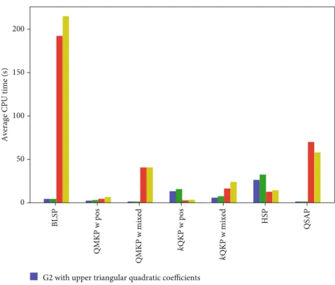
We report the average CPU times to solve the formula-tions to proven optimality for the diﬀerent BQP classes in Figure 4. As before, these average CPU times were computed after removing all instances where at least one of the formu-lations did not solve within the time limit.

Figure 4 provides some additional information not cap-tured in the performance profiles. First, note that while the performance profiles in Figure 3 indicate that G2 was supe-rior to G1, Figure 4 indicates that the actual difference in average solution times between G1 and G2 is fairly negligible when they are formulated with the same objective represen-tation. However, there are stark differences between the sym-metric and upper triangular coefficient representations for both G1 and G2. In particular, instances of G1 and G2 for-mulated with symmetric objective coefficients typically take considerably longer to solve on average than their respective models formulated with upper triangular coefficients. There are two exceptions—G2 with symmetric objective coefficients is superior for HSP and instances of kQKP with positive coefficients. 1 0.0 0.2 0.4 0.6

0.8 1.0

3

2 4 5

6 7

STD STD′

(g)

Figure_{1: Performance pro}_ﬁ_{les based on relative CPU time (s) for Question 1. (a) BLSP, (b) QMKP with positive coe}_ﬃ_{cients, (c) QMKP with}

mixed-sign coefficients, (d)kQKP with positive coefficients, (e)kQKP with mixed coefficients, (f) HSP, (g) QSAP.

0 BLSP QMKP w pos QMKP w mixed k QKP w Pos k QKP w mixed HSP QSAP 20 40 60 80 100

Average CPU time (s)

120 140

STD STD_′

(11)

1.0 0.0 0.2 0.4 0.6 C u m u la ti ve di st ri b u tio n fun ctio n 0.8 1.0 1.5 2.0 2.5 3.0 3.5 4.0 4.5 5.0

G2 with upper triangular quadratic coefficients G1 with upper triangular quadratic coefficients G2 with symmetric quadratic coefficients G1 with symmetric quadratic coefficients

(a) 1.0 0.0 0.2 0.4 0.6 C u m u la ti ve di st ri b u tio n fun ctio n 0.8 1.0 1.5 2.0 2.5 3.0 3.5 4.0 4.5 5.0

(b) 1.0 0.0 0.2 0.4 0.6 C u m u la ti ve di st ri b u tio n fun ctio n 0.8 1.0 1.5 2.0 2.5 3.0 3.5 4.0 4.5 5.0

(c) 1.0 0.0 0.2 0.4 0.6 C u m u la ti ve di st ri b u tio n fun ctio n 0.8 1.0 1.5 2.0 2.5 3.0 3.5 4.0 4.5 5.0

(d)

(12)

While the results are not completely definitive, Figures 3 and 4 indicate that in general, constraints (11) and (13) should be dropped from G1 to obtain G2 and the quadratic objective coefficients C should be represented in upper triangular form. We reiterate that while the average CPU time differences between G1 and G2 are fairly small, those differences are rather large for the two different objective function representations.

We now attempt to answer Question 5, which is con-cerned with whether it is advantageous to perform the substi-tution of variables that reduces G2 to either G2a or G2b. Figure 5 shows the performance proﬁles of G2, G2a, and

G3b where we aggregate across all objective coeﬃcient densi-ties, sizes, and MILP solvers. As with our previous test cases, we computed the bounds within the formulations as in (16). Note that, typically, G2 was the slowest formulation while G2a and G2b had fairly comparable likelihoods of being the fastest. Although, a closer examination reveals that G2a was slightly more likely to be the fastest formulation for all prob-lem classes except instances of QMKP with positive objective coeﬃcients. We report the average CPU times in Figure 6, which were computed as before.

While the average CPU times for G2, G2a, and G2b are all fairly similar for each problem classiﬁcation, G2a tended

1.0 0.0 0.2 0.4 0.6 C u m u la ti ve di st ri b u tio n fun ctio n 0.8 1.0 1.5 2.0 2.5 3.0 3.5 4.0 4.5 5.0

(e) 1.0 0.0 0.2 0.4 0.6 C u m u la ti ve di st ri b u tio n fun ctio n 0.8 1.0 1.5 2.0 2.5 3.0 3.5 4.0 4.5 5.0

(f) 1.0 0.0 0.2 0.4 0.6 C u m u la ti ve di st ri b u tio n fun ctio n 0.8 1.0 1.5 2.0 2.5 3.0 3.5 4.0 4.5 5.0

(g)

Figure_{3: Performance pro}_ﬁ_{les based on relative CPU time (s) for Questions 2 and 4. (a) BLSP, (b) QMKP with positive coe}_ﬃ_{cients, (c)}

(13)

to be the fastest formulation. Therefore, based on our tests, we recommend that G2 should be reduced in size via the sub-stitution of variablessj=U1jxj−zjto obtain G2a. While the

results were certainly not deﬁnitive, they do suggest that G2a has the highest probability of being the fastest formulation.

We now address Question 3 regarding how the bounds within Glover’s formulation should be computed. Within our tests, we refer to the bounds computed as in (15) asweak, those computed as in (16) astight, and those as in (17) as

tightest. Based upon our prior results, our tests were all per-formed using G2a formulated with the three diﬀerent methods to compute the bounds. We again reiterate that our solution times include not only the time to solve G2a to integer optimality but also the time required to compute the bounds within the formulation. Our results are presented in Figure 7 where we once again aggregate across all objective coeﬃcient densities, sizes, and MILP solvers. Note that we do not include the BLSP instances because for these problems, the bounds (15), (16), and (17) are all the same.

Interestingly, note that G2a formulated with the weak bounds of (15) tended to be the fastest formulation. We found this result surprising as preliminary experience showed that the tight bounds of (16) were superior. A more detailed analysis revealed that for smaller-sized instances, the extra time needed toﬁnd the tighter bounds of (16) was not warranted. However, once the instances start to become more challenging, the additional strength aﬀorded by the tight bounds (16) was advantageous even though the time

to ﬁnd the bounds increases. In order to better understand how these bounds aﬀect CPU time, let us examine the aver-age CPU times presented in Figure 8.

Note that in terms of average CPU times, G2a formulated with the tight bounds (16) was the best formulation for all problem classifications except instances ofkQKP with posi-tive objecposi-tive coefficients. Moreover, not only did the weak bounds (15) perform poorly in terms of average CPU times, they typically performed significantly worse than the tighter bounds. This stems from the fact that the continuous relaxa-tion strength of G2a formulated with (15) for anything other than smaller-sized instances is too weak for the linearization to be effective. Thus, our general recommendation is to for-mulate Glover’s model with the tight bounds of (16), espe-cially for larger-sized instances.

We summarize the answers and recommendations from Questions 1 through 5 in Table 1.

In conclusion, our recommendation based on a detailed computational study across five different classes of BQPs and three different MILP solvers is to implement Glover’s formulation using the concise version G2a with an upper tri-angular objective coefficient matrix C where the bounds within the formulation are computed as in (16).

4.3. Comparison of Exact Solution Methods.In this section, we compare our recommended versions of the standard lin-earization and Glover’s method, STD′, and G2a formulated with an upper triangular quadratic coeﬃcient matrixC and the bounds of (16), with the more recent linearization of

0 50 100

150 200 BLSP QMKP w pos QMKP w mixed k QKP w pos k QKP w mixed HSP QSAP

(14)

1.0 1.5 2.0 2.5 3.0 3.5 4.0 4.5 5.0

G2 G2a G2b

𝜏 = Factor of best ratio 0.0

0.2 0.4 0.6

0.8 1.0 (a) 1.0 1.5 2.0 2.5 3.0 3.5 4.0 4.5 5.0 G2 G2a G2b

0.2 0.4 0.6

0.8 1.0

(b)

1.0 1.5 2.0 2.5 3.0 3.5 4.0 4.5 5.0

0.2 0.4 0.6

0.8 1.0 G2 G2a G2b (c) 1.0 1.5 2.0 2.5 3.0 3.5 4.0 4.5 5.0 G2 G2a G2b

0.2 0.4 0.6

0.8 1.0 (d) 1.0 1.5 2.0 2.5 3.0 3.5 4.0 G2 G2a G2b

0.2 0.4 0.6

0.8 1.0 (e) 1.0 1.5 2.0 2.5 3.0 3.5 4.0 4.5 5.0 G2 G2a G2b

0.2 0.4 0.6

0.8 1.0

(f)

(15)

Sherali and Smith and direct submission to an optimization solver. When formulating the Sherali-Smith model, we uti-lized the bounds of (16) and an upper triangular quadratic coeﬃcient matrix.

As noted earlier, many MILP solvers have recently been updated to directly handle nonconvex BQPs. Before

examin-ing the results of our study, we review the two approaches typically utilized by commercial MILP solvers to solve non-convex BQPs directly. The MILP solvers of CPLEX, GUR-OBI, and XPRESS employ one of two diﬀerent strategies for solving nonconvex BQPs. Theﬁrst strategy consists of trans-forming the nonconvex problem into an equivalent convex

G2 G2a G2b

1.0 1.5 2.0 2.5 3.0 3.5 4.0 4.5 5.0

0.2 0.4 0.6

0.8 1.0

(g)

Figure_{5: Performance pro}_ﬁ_{les based on relative CPU time (s) for Question 5. (a) BLSP, (b) QMKP with positive coe}_ﬃ_{cients, (c) QMKP with}

mixed-sign coefficients, (d)kQKP with positive coefficients, (e)kQKP with mixed coefficients, (f) HSP, (g) QSAP.

BLSP QMKP w pos QMKP w mixed k QKP w pos k QKP w mixed HSP QSAP G2 G2a G2b

0 10 20 30 40 50 60

(16)

2 0.0 0.2 0.4 0.6 0.8 1.0 4 6 8 10 12 14 16 C u m u la ti ve di st ri b u ti o n fun ctio n

𝜏 = Factor of best ratio Weak bounds Tight bounds Tightest bounds (a) 2 0.0 0.2 0.4 0.6 0.8 1.0 4 6 8 10 12 14 16 C u m u la ti ve di st ri b u ti o n fun ctio n

𝜏 = Factor of best ratio Weak bounds Tight bounds Tightest bounds (b) 2 0.0 0.2 0.4 0.6 0.8 1.0 4 6 8 10 12 14 16 C u m u la ti ve di st ri b u ti o n fun ctio n

𝜏 = Factor of best ratio Weak bounds Tight bounds Tightest bounds (c) 2 0.0 0.2 0.4 0.6 0.8 1.0 4 6 8 10 12 14 C u m u la ti ve di st ri b u ti o n fun ctio n

𝜏 = Factor of best ratio Weak bounds Tight bounds Tightest bounds (d) 2 0.0 0.2 0.4 0.6 0.8 1.0 4 6 8 10 12 14 C u m u la ti ve di st ri b u ti o n fun ctio n

𝜏 = Factor of best ratio Weak bounds Tight bounds Tightest bounds (e) 0.0 1 2 3 4 5 6 7 8 9 10 0.2 0.4 0.6 0.8 1.0 C u m u la ti ve di st ri b u ti o n fun ctio n

𝜏 = Factor of best ratio Weak bounds

Tight bounds Tightest bounds

(f)

Figure_{7: Performance pro}_ﬁ_{les based on relative CPU time (s) for Question 3. (a) QMKP with positive coe}_ﬃ_{cients, (b) QMKP with}

(17)

BQP, which can then be solved using standard convex qua-dratic programming techniques. This is accomplished by using the identityx=xT_I_x _when_x_{is binary. The quadratic}

portion of the objective function xTCx can therefore be replaced by xT_ð_C₊_ρI_Þ_x₋_ρ_x_{. A number of strategies for}

selecting aρso thatC+ρIwill be negative semideﬁnite have been proposed, such as those by Billionet et al. [19]. The sec-ond strategy is to employ a linearization technique to trans-form the nonconvex BQP into an equivalent linear trans-form, such as the standard linearization.

For this second part of our computational study, we randomly generated a completely new set of test problems from those used in Sections 4.1 and 4.2. In addition, we also adjusted the sizes of the problem instances to include more challenging problems (although all other aspects of the instances were generated as presented in Section 3). With regards to instances of Problem QMKP with positive objec-tive coeﬃcients,nwas varied from 110 to 140 in increments of 10 whenk= 1and varied from 50 to 80 in increments of 10 when k= 5 or 10. For instances of QMKP with objective

QMKP w pos QMKP w mixed k QKP w pos k QKP w mixed HSP QSAP Weak bounds Tight bounds Tightest bounds

0 10 20 30 40 50

Figure_{8: Average CPU times (s) for Question 3.}

Table_{1: Summary of answers to Questions 1 through 5.}

Question Answer/recommendation

1: When applying the standard linearization to a BQP, should you reduce the size of the formulation based on the sign of the quadratic objective coeﬃcients?

Our recommendation is to use the sign-based formulation STD′ when using the standard linearization.

2: When applying Glover’s formulation, should you represent the quadratic objective coeﬃcient matrixCin upper triangular or symmetric form?

Our recommendation is to represent the quadratic objective coeﬃcient matrixCin upper triangular form when using Glover’s

method. 3: With regards to the overall computational eﬀort to formulate and

solve problem G1 to optimality using a MILP solver, should we compute the boundsU_j1,U_j0,L1_j, andL0_jusing (15), (16), or (17)?

In general, we recommend using the bounds of (16) when applying Glover’s method. However, for smaller-sized instances it may be

beneﬁcial to use the weaker bounds of (15). 4: How do formulations G1 and G2 compare when submitted to a

MILP solver? In general, formulation G2 is superior to G1.

5: Is it advantageous to perform the substitution of variables to reduce Problem G2 to G2a or G2b when submitting the model to a MILP solver?

While formulations G2, G2a, and G2b are fairly comparable in terms of performance, our general recommendation is to use G2a when

(18)

2 4 6 8 10 12 14

𝜏 = Factor of best ratio 0.0 0.2 0.4 0.6 0.8 1.0

G2a STD_′ SS

Quadratic submission to CPLEX Quadratic submission to GUROBI Quadratic submission to XPRESS

(a)

2 4 6 8 10 12 14

G2a STD′ SS

(b)

2 4 6 8 10 12 14

G2a STD′ SS

(c)

2 4 6 8 10 12 14

G2a STD′ SS

(d)

(19)

coeﬃcients of mixed sign, n was varied from 40 to 70 in increments of 10 fork= 1, 5, or 10. We variednfrom 20 to 50 in increments of 10 for Problem HSP. For instances of

kQKP with positive objective coeﬃcients,nwas varied from 60 to 90 in increments of 10, while for those instances with objective coeﬃcients of mixed sign, we variednfrom 80 to 110 in increments of 10. With regards to Problem QSAP, we considered ten ðm,nÞ pairs where n∈f4, 5g and m∈ f10, 12, 15, 18, 20g. For BLSP, we maintained the same sizes as before since this set was already challenging.

The performance proﬁles of our results are presented in Figure 9, where we once again aggregate across all objective coeﬃcient densities and sizes. Note that in order to ensure that the number of problem instancesnpis the same for each

of the formulations as required to construct performance proﬁles, we only solved the linearizations STD′, G2a, and SS with CPLEX, as opposed to all three solvers as in Sections 4.1 and 4.2. We report the average CPU times in Figure 10, which were computed as before. That is, these average CPU times were computed after removing all instances where at

2 4 6 8 10 12 14

G2a STD_′ SS

(e)

2 4 6 8 10 12 14

G2a STD′ SS

(f)

2 4 6 8 10 12 14

G2a STD′ SS

(g)

Figure_{9: Performance pro}_ﬁ_{les based on relative CPU time (s) for all approaches. (a) BLSP, (b) QMKP with positive coe}_ﬃ_{cients, (c) QMKP}

(20)

least one of the formulations did not solve within the time limit. Thus, the averages only include instances in which all formulations were solved to optimality within the 1-hour time limit.

While we had hoped that a single strategy would emerge as the best approach for solving all BQPs regardless of prob-lem class, the results presented in Figures 9 and 10 clearly indicate that this is not the case. Indeed, different strategies appear to be superior for each of the different problem clas-ses. We begin by noting that in general, direct submission of the BQP does not appear to be competitive with submis-sion of any of the linear reformulations. In fact, the average CPU times are typically much higher when using the qua-dratic solvers of CPLEX, GUROBI, and XPRESS as opposed to solving the linearizations. Moreover, the quadratic solvers were more likely to not be able to solve all instances. For example, the XPRESS solver was unable to solve approxi-mately 55% of the instances of QMKP with objective coefficients of mixed sign. Of the three solvers, CPLEX per-formed the best for direct submission, which is not surprising given that the nonconvex BQP solver of CPLEX is more mature than those of GUROBI or XPRESS (CPLEX has had the ability to solve nonconvex BQP well before GUROBI or XPRESS). Overall, our tests suggest that while it is convenient to be able to directly submit a BQP to the solver, solution times may be significantly reduced by reformulating the problem into linear form by the user before applying the solver.

We now examine the performance proﬁles of Figure 9 to compare the linearizations STD′, G2a, and SS. The standard linearization STD′ had the highest probability of being the

fastest formulation for instances of QMKP with objective coeﬃcients of mixed sign and instances of HSP. Glover’s lin-earization G2a had the highest probability of being the best formulation to solve instances of BLSP and instances of k

QKP with both positive objective coeﬃcients and objective coeﬃcients of mixed sign. The linearization of Sherali and Smith SS had the largest probability of being the fastest for-mulation for instances of QMKP with positive objective

coef-ficients, instances of kQKP with objective coefficients of mixed sign, and instances of QSAP. When examining the data a little more closely, G2a was the top performing formu-lation for instances of HSP that were 75% dense, instances of QMKP with objective coefficients of mixed sign that had den-sities of 75% and 100%, and instances ofkQKP with objective coefficients of mixed sign that were 100% dense.

In terms of the average CPU times in Figure 10, there were no signiﬁcant diﬀerences between the three lineariza-tions. All of the average solution times were fairly close with the exception of STD′applied to instances of QSAP. Indeed, STD′ performed poorly for this class of BQP.

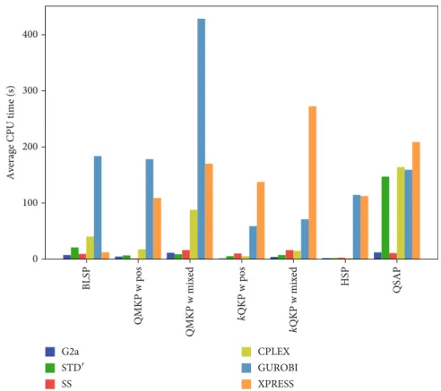
We end our analysis by aggregating the test results for all of the classes of BQPs into a single data set. The performance proﬁles of the three linearizations are presented in Figure 11, while the average CPU times are presented in Figure 12.

We can see that G2a had the fastest solution time approx-imately 26% of the time, STD′was the fastest reformulation approximately 38% of the time, while SS was the superior for-mulation approximately 34% of the time. Interestingly, in terms of average overall CPU time, we see a diﬀerent pattern. Note that STD′required an average overall CPU time of 70

BLSP QMKP w pos QMKP w mixed k QKP w pos k QKP w mixed HSP QSAP

0 100 200 300 400 G2a STD′ SS CPLEX GUROBI XPRESS

(21)

seconds, while G2a only required an average of 28 seconds. While we omit the details for brevity, a closer examination of the data suggests that STD′ is better suited for smaller-sized instances of BQPs, likely because of the large number of auxiliary variables and constraints. For larger-sized instances of BQPs, the compactness of G2a and SS seems to provide an advantage when submitted to an MILP solver.

5. Conclusions and Recommendations

In this paper, we revisited the standard linearization [3] and Glover’s method [4] for reformulating a BQP into linear form. Using a large-scale computational study overﬁve dif-ferent classes of BQPs, we evaluated a number of enhance-ments that have been proposed for these two linearizations.

0 10 20 30 40 50 60 70 G2a STD′ SS

Figure_{12: Average CPU times (s) over all problem classes.}

2 0.0 0.2 0.4 0.6 0.8 1.0 4 6 8 10 12 14

𝜏 = Factor of best ratio G2a

STD′ SS

(22)

Based on our analysis, we recommend that when reformulat-ing a BQP usreformulat-ing the standard linearization, the sign-based version STD′should be utilized. When applying Glover’s lin-earization, we recommend using the concise version G2a with an upper triangular objective coeﬃcient matrixCwhere the bounds within the formulation are computed as in (16). In the second part of our study, we compared the STD′ and G2a formulations with the more recent linearization of Sherali and Smith and direct submission of the BQP to the solver. Our analysis showed that while it is convenient to sub-mit a BQP directly to the solver, in general, it is advantageous for the user to perform a linear reformulation themselves beforehand. That being said, the more mature nonconvex BQP solver of CPLEX fared acceptably well on a number of diﬀerent problem classes. Among the linear reformulations studied, no linearization was superior over all problem clas-ses in terms of the probability of having the fastest solution times. In terms of overall average CPU time across all classes of BQPs, G2a and SS yielded the best times. Based upon our analysis, we recommend using STD′ for smaller-sized instances of BQPs, while for larger-sized instances, we rec-ommend using either G2a or SS.

Data Availability

The data used to support theﬁndings of this study are avail-able from the corresponding author upon request.

Conflicts of Interest

The authors declare that they have no conﬂicts of interest.

References

[1] R. Pörn, O. Nissfolk, A. Skjäl, and T. Westerlund,“Solving 0-1 quadratic programs by reformulation techniques,”Industrial & Engineering Chemistry Research, vol. 56, no. 45, pp. 13444–13453, 2017.

[2] G. Kochenberger, J. K. Hao, F. Glover et al., “The uncon-strained binary quadratic programming problem: a survey,” Journal of Combinatorial Optimization, vol. 28, no. 1, pp. 58–81, 2014.

[3] F. Glover and E. Woolsey,“Technical Note—Converting the 0-1 polynomial programming problem to a 0-1 linear pro-gram,”Operations Research, vol. 22, no. 1, pp. 180–182, 1974. [4] F. Glover, “Improved linear integer programming formula-tions of nonlinear integer Problems,” Management Science, vol. 22, no. 4, pp. 455–460, 1975.

[5] H. D. Sherali and J. C. Smith, “An improved linearization strategy for zero-one quadratic programming problems,”

Opti-mization Letters, vol. 1, no. 1, pp. 33–47, 2007.

[6] R. M. Lima and I. E. Grossmann,“On the solution of noncon-vex cardinality Boolean quadratic programming problems: a computational study,” Computational Optimization and

Applications, vol. 66, no. 1, pp. 1–37, 2017.

[7] F. Furini and E. Traversi, “Theoretical and computational study of several linearisation techniques for binary quadratic problems,”Annals of Operations Research, vol. 279, no. 1-2, pp. 387–411, 2019.

[8] R. Forrester and H. Greenberg,“Quadratic binary program-ming models in computational biology,”Algorithmic

Opera-tions Research, vol. 3, pp. 110–129, 2008.

[9] W. P. Adams, R. J. Forrester, and F. W. Glover,“Comparisons and enhancement strategies for linearizing mixed 0-1 qua-dratic programs,” Discrete Optimization, vol. 1, no. 2, pp. 99–120, 2004.

[10] R. J. Forrester, W. P. Adams, and P. T. Hadavas,“Concise RLT forms of binary programs: a computational study of the qua-dratic knapsack problem,” Naval Research Logistics, vol. 57, no. 1, pp. 1–12, 2010.

[11] W. P. Adams and R. J. Forrester,“A simple recipe for concise mixed 0-1 linearizations,” Operations Research Letters, vol. 33, no. 1, pp. 55–61, 2005.

[12] H. Wang, G. Kochenberger, and F. Glover,“A computational study on the quadratic knapsack problem with multiple con-straints,”Computers and Operations Research, vol. 39, no. 1, pp. 3–11, 2012.

[13] D. Pisinger, “The quadratic knapsack problem—a survey,”

Discrete Applied Mathematics, vol. 155, no. 5, pp. 623–648,

2007.

[14] A. Billionnet,“Diﬀerent formulations for solving the Heaviest

K-Subgraph problem,”INFOR: Information Systems and

Oper-ational Research, vol. 43, no. 3, pp. 171–186, 2005.

[15] L. Létocart, M. C. Plateau, and G. Plateau,“An eﬃcient hybrid heuristic method for the 0-1 exactk-item quadratic knapsack problem,” Pesquisa Operacional, vol. 34, no. 1, pp. 49–72, 2014.

[16] L. Létocart and A. Wiegele, “Exact solution methods for the

k-item quadratic knapsack problem,” inInternational

Sym-posium on Combinatorial Optimization, pp. 166–176,

Springer, Cham, 2016.

[17] A. Billionnet, S. Elloumi, and M.-C. Plateau,“Improving the performance of standard solvers for quadratic 0-1 programs by a tight convex reformulation: The QCR method,”Discrete

Applied Mathematics, vol. 157, no. 6, pp. 1185–1197, 2009.

[18] E. D. Dolan and J. J. Moré,“Benchmarking optimization soft-ware with performance proﬁles,”Mathematical Programming, vol. 91, no. 2, pp. 201–213, 2002.

[19] A. Billionnet, S. Elloumi, and A. Lambert,“Extending the QCR method to general mixed-integer programs,” Mathematical