Quick Switching Conditional RGS Plan 3 Indexed through Outgoing Quality Levels

(1)

Quick Switching Conditional RGS Plan-3 Indexed

through Outgoing Quality Levels

V. Kaviyarasu

Department of Statistics, Bharathiar University, Coimbatore, Tamil Nadu, India *Corresponding Author:[email protected]

Abstract

This paper tries to study the designing of new attribute sampling plan towards Quick Switching Conditional Repetitive Group Sampling System (QSCRGSS)-3 indexed through Average Outgoing Quality (AOQ), Average Outgoing Quality Limit (AOQL) and its Operating Ratio (OR). Tables are provided with numerical illustrations for newly developed plan for its various plan parameters.

Keyword

Quick Switching System, Conditional Repetitive Group Sampling Plan, AOQ, AOQL and Operating Ratio

1. Introduction

Statistical Quality Control is widely used in industry to ensure customer satisfaction due to mass production of products and services. Acceptance sampling was widely used to test the quality of the product towards reduction of variability in process and product where variation is measured by statistical methods. An important field of statistical quality control is acceptance sampling which is either to accept or reject products of a lot under sample inspection when 100% inspection is not possible. The primary objective of sampling inspection is to reduce the cost of inspection while at the same time assuring the customer to an adequate level of quality for the items being inspected under identical conditions for both the producer and consumer.

This paper presents a new repetitive sampling plan for attributes which has considered by base and reference sampling plan. The Quick Switching System (QSS) as base plan and Conditional Repetitive Group Sampling Plan as reference plan to propose a new sampling plan called as Quick Switching Conditional Repetitive Group Sampling System (QSCRGSS)-3. Sampling plan is widely used in government sector and industry for controlling the quality of shipment of components, supplies and final products (e.g. life of electric bulbs, tensil strength and hardness of steel casting etc.,). Similar situations can be thought over the time

where the quality of the product improves with decrease in the value of inspection cost.

2. Quick Switching System

Dodge (1967) proposed a new sampling inspection plan involving normal and tightened inspection which is usually referred as two-plan system. Romboski (1969) studies a Quick Switching System, switching to tightened inspection when the rejection comes under normal inspection. Due to instantaneous switching between normal and tightened plans, this system is referred as ‘Quick Switching System (QSS)’. Romboski (1969) has further studied the merits and demerits of switching rules of QSS when it is compared with two-plan system (m, d). The rule of QSS is retained at m=1 where as tightened rule is made when d>1.Two natural choice for tightened rule for d=2, d=3 etc., which are designed as QSS-2, QSS-3 and QSS-d. Schilling (1981) has mentioned the switching rules employed in the system are simple and the condition for application has evolved.

3. Conditional Repetitive Group

Sampling (CRGS) Plan

The concept of Repetitive Group Sampling (RGS) plan was introduced by Sherman (1965) in which acceptance or rejection of a lot is based on the repeated sample results on the same lot. Soundararajan and Ramasamy (1986) has tabulated the values for selection of RGS plan indexed through (AQL, AOQL), (p0, h0) and (p*, h*). Gauri shankar

and Mohapatra (1993) has developed a new Repetitive Group Sampling plan designated as Conditional Repetitive Group Sampling plan in which disposal of lot on the basis of repeated sample results is dependent on the outcome of the inspection of the immediate preceding i lots. Further they derived the formulae for OC and ASN function.

(2)

Quality Level (AQL), Limiting Quality Level (LQL), Indifference Quality Level (IQL) and AOQL. This paper provides a new procedure for selection of QSS-3 with Conditional RGS plan indexed through outgoing quality levels, which are tailor made for industrial shop floor applications.

4. Designation

QSCRGSS-3 (n; u1, u2; v1, v2) refers to a Quick Switching

System of type 3 where the normal CRGS plan has a sample size n and acceptance number u1, u2 (u1 < u2) and the

tightened CRGS plan has a sample size n and acceptance number v1, v2 (v1< v2, v1≤ u1 and v2 ≤ u2). The plan has six

parameters namely n, u1, u2; v1, v2and i.

5. Operating Procedure

The Quick Switching Conditional Repetitive Group Sampling plan-3 is carried out through the following steps: Step 1: Draw a random sample of size n and test each unit for its conformation for the specified requirements.

Step 2: Under normal inspection, inspect the plan under Conditional Repetitive Group Sampling plan with the parameters n,

u1and u2. If lot is accepted, continue step 2 otherwise

step 3.

Step3: Under tightened inspection, inspect the plan under Conditional Repetitive Group Sampling plan with the parameters n,

v1 and v2. If a lot is accepted, Continue step 3 for next 3 lots and goes to step 2, otherwise step 3.

Thus, the Quick Switching Conditional Repetitive Group Sampling Systems (QSCRGSS)-3 are characterized with six parameters namely, n, u1, u2, v1, v2, and i. Here, it may be

observed that when u1 = u2 = v1 = v2, and i = 0 the resulting

plan is reduced to Repetitive Group Sampling plan due to Sherman (1965). Further, the Quick Switching Conditional Repetitive Group Sampling plan-3 is applicable to a stream of lots and not for isolated lots.

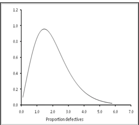
6. Operating Characteristics Function

Based on Sherman (1965), Romboski (1969), Arumainayagam (1991) and Jayalakshmi (2009) the expression for OC function of QSCRGSS-3 is given by,

Pa (p) =

(

)(

)

(

N

)(

T

)

T T N T T N

P

+

−

+

−

+

1

3 3 (1) Where, PN =

(

)

(

)

[

2 1

]

1 1 ) ( u X P u X p u X P r r r ≤ + ≤ −

≤ ₍₂₎

And

PT =

[

(

)

(

)

]

1 2 1

1 )

(

v

X

P

v

X

p

v

X

P

r r r

≤

+

≤

−

≤

(3) Glossary N = lot size n = sample size

p = incoming quality of the submitted lot Pa (p) = Probability of Acceptance

PN = probability of acceptance under normal inspection

PT = probability of acceptance under tightened inspection

u1 and u2 = acceptance numbers under normal inspection v1 and v2 = acceptance numbers under tightened inspection

α = Consumer risk and β = producer risk

P0.95, P0.50 = the lot or process quality for which the

probability of acceptance is 0.95 and 0.50 etc., for given sampling plan

i = clearance interval

PL = Average Outgoing Quality Limit (AOQL) and

Pm = Quality at which AOQL occurs.

7. Designing QSCRGSS-3 for Different

Parameters

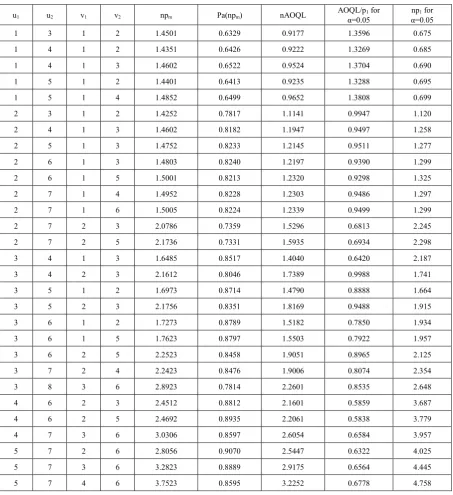
[image:2.595.319.544.463.665.2]

7.1. Designing Systems for given AQL and AOQL

(3)

[image:3.595.79.535.132.668.2]

Table 2 can be used to design a QSCRGSS-3 indexed by AQL and AOQL. For example, given AQL = 5.1% (α= 0.05) and AOQL = 7.04% one can compute AOQL / AQL = 7.04 / 5.1 = 1.38039. From the table 1 the value of AOQL / AQL closest to the desired value is 1.3704. This value corresponds to u1 = 1, u2 = 4, v1 = 1, v2 = 3, i = 2 and np1 = 0.690.

Table 1. AOQL values for QSCRGSS-3 when i = 1

u1 u2 v1 v2 npm Pa(npm) nAOQL _{for α=0.05}AOQL/p1 _α=0.05np1 for

1 3 1 2 1.4701 0.6802 1.0000 1.2706 0.787

1 4 1 2 1.4601 0.6944 1.0140 1.2291 0.825

1 4 1 3 1.5501 0.6928 1.0740 1.2431 0.864

1 5 1 2 1.4601 0.6976 1.0186 1.2272 0.830

1 5 1 4 1.6001 0.6907 1.1052 1.2335 0.896

2 3 1 2 1.5051 0.7892 1.1879 0.9999 1.188

2 4 1 3 1.6051 0.8272 1.3278 0.9594 1.384

2 5 1 3 1.6301 0.8382 1.3663 0.9745 1.402

2 6 1 3 1.6401 0.8405 1.3786 0.9296 1.483

2 6 1 5 1.6901 0.8347 1.4107 0.9275 1.521

2 7 1 4 1.6801 0.8365 1.4053 1.0356 1.357

2 7 1 6 1.7001 0.8331 1.4164 0.9455 1.498

2 7 2 3 2.1601 0.7717 1.6669 1.0938 1.524

2 7 2 5 2.3451 0.7603 1.7830 1.0999 1.621

3 4 1 3 1.7601 0.8527 1.5008 0.8566 1.752

3 4 2 3 2.2551 0.8070 1.8198 1.0065 1.808

3 5 1 2 1.8022 0.8769 1.5803 0.8863 1.783

3 5 2 3 2.2972 0.8431 1.9368 0.9402 2.060

3 6 1 2 1.8561 0.8869 1.6462 0.7303 2.254

3 6 1 5 1.9461 0.8878 1.7277 0.7621 2.267

3 6 2 5 2.4661 0.8534 2.1046 0.8566 2.457

3 7 2 4 2.4361 0.8597 2.0943 0.7361 2.845

3 8 3 6 3.1061 0.8010 2.4880 1.1082 2.245

4 6 2 3 2.5761 0.8825 2.2735 0.6987 3.254

4 6 2 5 2.6861 0.8844 2.3757 0.6502 3.654

4 7 3 6 3.2711 0.8645 2.8280 0.7545 3.748

5 7 2 6 2.9951 0.9061 2.7140 0.6380 4.254

5 7 3 6 3.4936 0.8877 3.1011 0.7116 4.358

(4)

[image:4.595.79.533.85.581.2]

Table 2. AOQL values for QSCRGSS-3 when i = 2

u1 u2 v1 v2 npm Pa(npm) nAOQL AOQL/p_α=0.051 for _α=0.05np1 for

1 3 1 2 1.4501 0.6329 0.9177 1.3596 0.675

1 4 1 2 1.4351 0.6426 0.9222 1.3269 0.685

1 4 1 3 1.4602 0.6522 0.9524 1.3704 0.690

1 5 1 2 1.4401 0.6413 0.9235 1.3288 0.695

1 5 1 4 1.4852 0.6499 0.9652 1.3808 0.699

2 3 1 2 1.4252 0.7817 1.1141 0.9947 1.120

2 4 1 3 1.4602 0.8182 1.1947 0.9497 1.258

2 5 1 3 1.4752 0.8233 1.2145 0.9511 1.277

2 6 1 3 1.4803 0.8240 1.2197 0.9390 1.299

2 6 1 5 1.5001 0.8213 1.2320 0.9298 1.325

2 7 1 4 1.4952 0.8228 1.2303 0.9486 1.297

2 7 1 6 1.5005 0.8224 1.2339 0.9499 1.299

2 7 2 3 2.0786 0.7359 1.5296 0.6813 2.245

2 7 2 5 2.1736 0.7331 1.5935 0.6934 2.298

3 4 1 3 1.6485 0.8517 1.4040 0.6420 2.187

3 4 2 3 2.1612 0.8046 1.7389 0.9988 1.741

3 5 1 2 1.6973 0.8714 1.4790 0.8888 1.664

3 5 2 3 2.1756 0.8351 1.8169 0.9488 1.915

3 6 1 2 1.7273 0.8789 1.5182 0.7850 1.934

3 6 1 5 1.7623 0.8797 1.5503 0.7922 1.957

3 6 2 5 2.2523 0.8458 1.9051 0.8965 2.125

3 7 2 4 2.2423 0.8476 1.9006 0.8074 2.354

3 8 3 6 2.8923 0.7814 2.2601 0.8535 2.648

4 6 2 3 2.4512 0.8812 2.1601 0.5859 3.687

4 6 2 5 2.4692 0.8935 2.2061 0.5838 3.779

4 7 3 6 3.0306 0.8597 2.6054 0.6584 3.957

5 7 2 6 2.8056 0.9070 2.5447 0.6322 4.025

5 7 3 6 3.2823 0.8889 2.9175 0.6564 4.445

5 7 4 6 3.7523 0.8595 3.2252 0.6778 4.758

7.2. Determining the value of AOQL of a given system

Table 1 can be used to obtain the values of AOQL and pm for a given system. For example, QSCRGSS-3(63; 3, 8; 3, 6)

when i = 1, from table 1, corresponding to these entry plan parameters one can get nAOQL = 2.4880 and npm = 3.1061. So

AOQL = nAOQL / n = 2.4880 / 63 = 0.03949 and pm = npm / n = 3.1061 / 63 = 0.04930.

7.3. Conversion from one set of parameters to the other

Table 1 can be used to convert the given set of parameters to another familiar equivalent set. For example, for given AQL = 0.05, α = 0.05, LQL = 0.09 and β = 0.10, from the Table one can fix the QSCRGSS-3 plan as n = 55, u1 = 3, u2 = 4, v1 = 2, v2 = 3 when i = 1. Corresponding to these entry parameters, one can find the following values from tables.

np1 = 1.808 npm = 2.2551 nAOQL = 1.8198

np0 = 2.2954 h0 = 1.8461

(5)

AQL (α = 0.05) = 0.05, AOQL = nAOQL / n = 1.8198 / 55 = 0.03308 IQL = np0 / n = 2.2954 / 55 = 0.04173

Thus, for given (AQL, 1-α) and (LQL, β), other equivalent parameters were (AQL, AOQL) and (p0, h0) are (0.05, 0.03308)

and (0.04173, 1.8461).

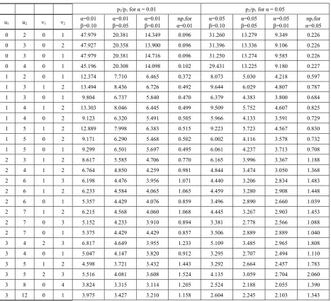
7.4. Designing Systems given p1, α, p2 and β

Table 3 can be used to design Quick Switching Conditional Repetitive Group Sampling System (QSCRGSS)-3, when two points on the OC curve (p1, 1- α) and (p2, β) are given. To design a QSCRGSS-3 the operating ratio (OR) = p2 / p1. From table

3, one can determine the value of OR which is nearer to the desired ratio. Corresponding to the selected OR values of u1, u2, v1, v2 and np1 when i = 1. The sample size is determined by dividing np1 by p1.

For example, let p1 = 0.05, α = 0.05, p2 = 0.395 and β = 0.10, calculate the Operating Ratio (OR) = p2 / p1 = 0.395 / 0.05 =

7.9. From the table 3 the value of OR for α = 0.05 and β = 0.10 which is the nearest to the desired ratio is 8.0731. Corresponding to this selected OR values are u1 = 1, u2 = 2, v1 = 0, v2 = 1 when i = 1 and np1 = 0.372. The sample size is

obtained as n = np1 / p1 = 0.372 / 0.05 = 7.44 ~ 7. The desired system is QSCRGSS-3(7; 1, 2) for normal and (7; 0, 1) for

[image:5.595.73.541.286.711.2]

tightened case when i = 1.

Table 3. Operating Ratio values for QSCRGSS-3 (n, u1, u2, v1, v2) when i=1

p2/p1 for α = 0.01 p2/p1 for α = 0.05

u1 u2 v1 v2 α=0.01 _β=0.10 α=0.01 _β=0.05 α=0.01 _β=0.01 _α=0.01np1for α=0.05 _β=0.10 α=0.05 _β=0.05 α=0.05 _β=0.01 _α=0.05np1for

0 2 0 1 47.979 20.381 14.349 0.096 31.260 13.279 9.349 0.226

0 3 0 2 47.927 20.358 13.900 0.096 31.396 13.336 9.106 0.226

0 3 0 1 47.979 20.381 14.716 0.096 31.250 13.274 9.585 0.226

0 4 0 1 45.196 20.308 14.098 0.102 29.431 13.225 9.180 0.227

1 2 0 1 12.374 7.710 6.465 0.372 8.073 5.030 4.218 0.597

1 3 1 2 13.494 8.436 6.726 0.492 9.644 6.029 4.807 0.787

1 3 0 1 9.804 6.737 5.840 0.470 6.379 4.383 3.800 0.684

1 4 1 2 13.303 8.046 6.445 0.499 9.509 5.752 4.607 0.825

1 4 0 2 9.123 6.320 5.491 0.505 5.966 4.133 3.591 0.729

1 5 1 2 12.889 7.998 6.383 0.515 9.223 5.723 4.567 0.830

1 5 0 2 9.171 6.290 5.468 0.502 6.002 4.116 3.578 0.732

1 5 0 1 9.299 6.501 5.697 0.495 6.061 4.237 3.713 0.708

2 3 1 2 8.617 5.585 4.706 0.770 6.165 3.996 3.367 1.188

2 4 1 2 6.764 4.850 4.259 0.981 4.844 3.474 3.050 1.368

2 6 1 3 6.198 4.476 3.956 1.071 4.440 3.206 2.834 1.483

2 6 1 2 6.233 4.584 4.065 1.065 4.459 3.280 2.908 1.448

2 6 0 1 5.357 4.429 4.076 0.859 3.496 2.890 2.660 1.039

2 7 1 2 6.215 4.568 4.060 1.068 4.445 3.267 2.903 1.453

2 7 0 3 5.152 4.233 3.910 0.894 3.381 2.778 2.566 1.088

2 7 0 1 5.375 4.429 4.429 0.857 3.506 2.889 2.889 1.040

3 4 2 3 6.817 4.649 3.955 1.233 5.109 3.485 2.965 1.808

3 4 0 1 5.047 4.147 3.820 0.912 3.295 2.707 2.494 1.110

3 5 1 2 4.598 3.721 3.432 1.443 3.292 2.664 2.457 1.783

3 5 2 3 5.516 4.081 3.608 1.524 4.135 3.059 2.704 2.060

3 8 0 4 3.824 3.315 3.114 1.205 2.524 2.188 2.055 1.390

(6)

[image:6.595.71.541.93.592.2]

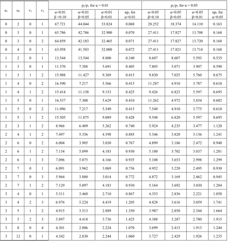
Table 4. Operating Ratio values for QSCRGSS-3 (n, u1, u2, v1, v2) when i=2

u1 u2 v1 v2

p2/p1 for α = 0.01 p2/p1 for α = 0.05

α=0.01

β =0.10 α=0.01 β=0.05 α=0.01 β=0.01 α=0.01 np1 for α=0.05 β=0.10 α=0.05 β=0.05 α=0.05 β=0.01 α=0.05 np1 for 0 2 0 1 67.721 44.044 33.824 0.068 28.252 18.374 14.110 0.163 0 3 0 1 65.786 42.786 32.900 0.070 27.411 17.827 13.708 0.168 0 3 0 2 64.859 42.183 32.465 0.071 27.411 17.827 13.720 0.168 0 4 0 1 63.958 41.583 32.000 0.072 27.411 17.821 13.714 0.168

1 2 0 1 13.544 13.544 8.800 0.340 8.607 8.607 5.593 0.535

1 3 0 1 11.370 7.388 5.691 0.405 7.805 5.071 3.907 0.590

1 3 1 2 15.988 11.427 9.369 0.415 9.830 7.025 5.760 0.675

1 4 0 2 16.590 7.217 5.566 0.415 11.287 4.910 3.787 0.610

1 4 1 2 15.414 11.158 9.153 0.425 9.426 6.823 5.597 0.695

1 5 0 1 16.537 7.300 5.629 0.410 11.262 4.972 3.834 0.602

1 5 0 2 11.096 7.217 5.549 0.415 7.549 4.910 3.775 0.610

1 5 1 2 15.505 11.075 9.089 0.428 9.548 6.820 5.597 0.695

2 3 1 2 8.966 6.409 5.262 0.740 5.924 4.235 3.477 1.120

2 4 1 2 7.497 5.356 4.398 0.885 5.346 3.820 3.136 1.241

2 6 0 2 6.004 3.905 3.030 0.767 4.899 3.186 2.472 0.940

2 6 1 2 7.134 5.099 4.183 0.930 5.180 3.702 3.037 1.281

2 6 1 3 7.096 5.075 4.166 0.935 5.108 3.653 2.998 1.299

2 7 0 1 6.091 3.962 3.069 0.756 4.952 3.220 2.495 0.930

2 7 0 3 5.964 3.880 3.014 0.772 4.872 3.169 2.462 0.945

2 7 1 2 7.129 5.097 4.183 0.930 5.164 3.692 3.030 1.284

3 4 0 1 5.311 3.460 2.710 0.867 4.353 2.836 2.221 1.058

3 4 2 3 6.976 5.224 4.419 1.205 4.828 3.616 3.059 1.741

3 5 1 2 4.915 3.513 2.889 1.350 3.987 2.850 2.344 1.664

3 5 2 3 5.897 4.418 3.736 1.425 4.388 3.287 2.780 1.915

3 8 0 4 4.301 2.806 2.224 1.070 3.699 2.413 1.913 1.244

3 12 0 1 4.342 2.830 2.244 1.060 3.727 2.429 1.926 1.235

7.5. Operating Ratio

Designing Systems for given Operating Ratio

Table 3 and 4 can be used to design QSRGSS-3, when two points on the OC curve (p1, 1- α) and (p2, β) are given.

To design a QSRGSS-3 calculate the Operating Ratio (OR) = p2 / p1. From table 3 and 4, one can determine the value of

OR which is nearer to the desired ratio, corresponding to the selected OR values of u1, u2, v1, v2, i and np1. The

sample size is determined by dividing np1 by p1.

For example, let p1 = 0.02, α = 0.05, p2 = 0.086 and β =

0.10, calculate the Operating Ratio (OR) = p2 / p1 = 0.086 /

0.02 = 4.3. From table 2.5.1, the value of OR for α = 0.05 and β = 0.05 which is the nearest to the desired ratio is 4.3424. Corresponding to this selected OR the parameters are u1 = 1, u2 = 3, v1 = 1, v2 = 2 and np1 = 1.1191. The

sample size is obtained as n = np1 / p1 = 1.1191 / 0.02 =

55.955 ≅ 56. The desired system is QSRGSS-3(56; 1, 3; 1, 2).

7.6. Construction of Tables

(7)

composite OC function is given by equation (1) with

PN =

( )

u

( )

i

x x np u x u x x np x np u o x x np x np e x np e x np e x np e             − +

∑

= − = = − − = − 1 1 2 1 0 0 0 ! / ! / ! / 1 ! / (4)

PT =

( )

v

( )

i

x x np v x v x x np x np v o x x np x np e x np e x np e x np e             − +

∑

= − = = − − = − 1 1 2 1 0

0 / ! 0 / ! / !

1

!

/

(5) For various assumed values of u1, u2, v1, v2, i and Pa (p) the

equation (1) is solved with the equation (4) and (5) one can get the np using iteration techniques from c++ computer program and values are obtained. Utilizing the np values tabulated for different values of u1, u2, v1, v2 and i. From table

1 and 2 the various outgoing quality levels and Operating Ratio values are calculated for different α and β values are given in table 3 and 4. Assuming nAOQ = np * Pa(p), value of np which maximizes nAOQ was obtained by the method of successive approximation and these values (npm) together

with nAOQL( = npm*Pa(pm)) appear in table 1 to 2.

8. Conclusion

Acceptance sampling is a technique which gives a better solution to the problems faced by the industry. Acceptance sampling itself does not improve quality, but whenever the lot is rejected it indicates the instability of the production process. Acceptance sampling is a cost efficient one and only an admissible method which is used for destructive and costly tests which provides quick results. Sampling plans are necessary to provide the disposal of defective products made, while efforts are activated to control the process. In that Quick Switching System and Conditional RGS Plan have wide potential applicability in industries to ensure a high standard of quality attainment and increased customer satisfaction. Here, an attempt is made towards the concept of Quick Switching Conditional Repetitive Group Sampling System (QSCRGSS)-3 in which disposal of a lot is on the basis of normal and tightened plans. Poisson unity values have been tabulated for a wide range of plan parameters. The present development would be valuable addition in the literature and a useful device to the quality practitioners. The concept of this article may be of assistance to quality control engineers and plan designers in the development of further plans.

REFERENCES

[1] AMERICAN NATIONAL STANDARDS,

Institute/American Society for Quality Control (ANSI/ASQC) STANDARD A2 (1987): “Terms, symbols and Definition for Acceptance Sampling”, American Society for Quality Control, Milwaukee, Wisconsin. USA.

[2] ARUMAINAYAGAM, S. D. (1991): “Contribution to the Study of Quick Switching System and its Application”, Ph.D., Thesis, Department of Statistics, Bharathiar University Coimbatore, Tamilnadu, India.

[3] DODGE, H. F. (1967): Notes on the Evolution of Acceptance Sampling Plans, Journal of Quality Technology. Vol.1, No.2, pp. 77-88.

[4] GAURI SANKAR and MOHAPATRA, B. N. (1993): GERT Analysis of Conditional Repetitive Group Sampling Plan,

International Journal of Quality & Reliability Management,

Vol.10, No.2, pp 50-62.

[5] GAURI SANKAR and JOSEPH, S. (1994): GERT Analysis of Multiple Repetitive Group Sampling Plans, IAPQR

Transactions, Vol.19, No.2, pp. 7-19.

[6] JAYALAKSHMI, S. (2009): Contribution to the Selection of Quick Switching System and related sampling plans, Ph.D Thesis, Department of Statistics, Bharathiar University, Coimbatore, Tamil Nadu, India.

[7] KAVIYARASU, V. and SURESH, K. K. (2011): Certain Results and Tables Relating to QSS-1 with Multiple RGS Plan, Journal of Mathematical Research, Canadian Center

of Science and Education, Canada Vol.3, No.4, pp.158-167,

Nov 2011.

[8] ROMBOSKI, L. D. (1969): “An Investigation of Quick Switching Acceptance Sampling Systems”, Ph.D Thesis, Rutgers- The State University, New Brunswick, New Jersey. [9] SCHILLING, E. G. (1981): A modified general procedure for sampling inspection, Frontiers in Statistical Quality Control, Edited Lenz, H.J., Wetherill, G.B., Wilrich, P.Th. Wilrich. [10] SHERMAN, R. E. (1965): “Design and Evaluation of

Repetitive Group Sampling Plans”, Technometrics, Vol.7, No.1, pp.11-21.

[11] SOUNDARARAJAN, V. and RAMASAMY, M. M. (1986): Procedures and Tables for Construction and Selection of Repetitive Group Sampling (RGS) Plan, the QR Journal, Vol.13, No.3, pp.19-21.