Assessment of the Combined Approach for the Environmental Impact of Water Purification System Study

(1)

Assessment of the Combined Approach for the

Environmental Impact of Water Purification

System Study

Lovorka Gotal Dmitrovic

1,*

_{, Ivica Mustac}

1

_{, Renata Bagnall}

2

1_{University Centre Varazdin, University North, Croatia} 2_{The Open University, Milton Keynes Campus, United Kingdom}

Abstract

The combined approach principle involves reducing water pollution from point and diffused sources. The objective of the combined approach is to reduce water pollution. The combined approach principle considers the quality of wastewater discharged into the receiver and their impact on the receiver. The methodology involves determining the flow of the receiver and effluent flow as well as determining the emission limit values (load of pollutants in the effluent). According to the type of receiver and depending on the discharge of effluent into streams, stagnant or into transitional and coastal waters, daily and annual load values permitted shall be determined. However, to obtain accurate values modelling methods must be used whose combined approaches solve the system of differential-difference equations.

Keywords

Combined Approach, Water Purification System

1. Introduction

The combined approach principle has been defined by the Article 58 of the Water Resources Act (NN No. 153/09, 63/11, 130/11, 63/11, 130/11, 56/13 and 14/14). The principle of the combined approach involves reducing water pollution from point and diffused sources. The methodology involves determining the flow of the receiver and effluent flow as well as determining the emission limit values (load of pollutants in the effluent):

(1)

whereas:

cds – downstream concentration of a pollutant in receiver

(river) (mg/l),

cus – upstream concentration of a pollutant in receiver

(river) (mg/l),

celv – emission limit value of a pollutant concentration in

river (mg/l),

Qds – downstream flow in receiver (river) (m3/s),

Qus – upstream flow in receiver (river) (m3/s),

Qef – effluent flow (m3/s)

According to the type of receiver and depending on the discharge of effluent into streams, stagnant or into transitional and coastal waters, daily and annual load values permitted shall be determined. In cases where the required water status cannot be achieved the additional protective measures and stricter conditions of discharge shall be regulated. However, to obtain accurate values must be used modelling methods which combined approach solves the differential system-differential equations.

The goal of the simulation modelling is purification wastewater optimisation process and methodology design suitable to significant behaviour patterns of contamination matter. Mathematical models for the modelling and analysing system, such as models of differential equations in continuous time models of differential equations with discrete time, the techniques of operations research and simulation models of discrete events, are well described in the literature, but the overall analysis behaviour of environmental systems includes a dynamic approach [2, 4].

(2)

Environment and Ecology Research 4(3): 140-145, 2016 141

the development of continuous and discrete systems models, the mechanism of the transition from one to the other components stage assures correct choice for model designing [2, 9].

Also, simulation modelling can display the system at various levels. Conceptual models offer a presentation given to the lawfulness of its behaviour and structure, and thus allow the study of the most important parameters of the functioning of the entire system or its components. Using mathematical, statistical and algorithmic presentation systems, allows exploring the legality of the system behaviour, as well as the interdependence of its entities and the development of systematic dynamics model of the system. In this way, simulation modelling is a powerful tool for analysing the state system, alignment parameters and the selection of the appropriate mode of operation of environmental systems.

The focus of this paper is modelling the purifying systems for wastewater with acceptable work for effluent discharge into the recipient. In order to make the systems work in optimal conditions that are based on the concentrations of pollution data, receiver flow and effluent flow changes with time. The designing of a conceptual as well as a mathematical model was required. These models can show the reduction in the observed pollutants concentration, by using the systems of differential-difference equations for the purifiers considered, along with function equations for each substance.

Following the mathematical model functions work development, it was necessary to design a computer model as well. Mathematical functions present independent variables, while the water quality in the supplied water purification systems, presents a dependent variable.

Searching the literature examples were found of using a combined approach, however, the main innovation and originality of this research, is that the original equation of the combined approach converted into system of differential equations, and to observe changes in the concentration and flow depending on the time.

2. The Conceptual Model

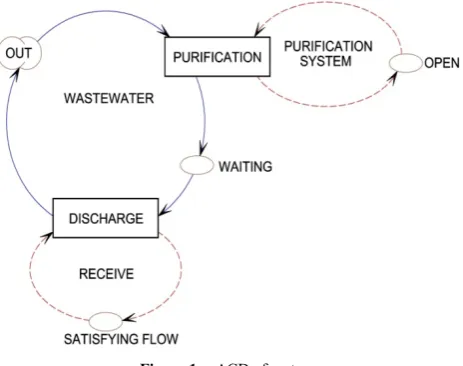
The conceptual model of system in the Diagram cycle activity - DCA (or Activity cycle diagram - ACD) form was created (Figure 1), as well as Ishikawa diagram (Figure 2).

There are many known modelling paradigms to describe the dynamics of system in process-oriented, based and activity-based viewpoints. Among those modelling paradigms, the activity-based modelling is a natural way to represent the activity paradigm of discrete event simulation and our knowledge about system components patterns behaviour. In activity-based modelling the dynamics of system is represented as an ACD (activity cycle diagram), which is a network model of the logical and temporal relationships among the activities [11]. An ACD is easily implemented with the activity scanning method of

simulation execution [11].

The activity cycle diagram (ACD) is a method to describe the interactions of objects in a system. It uses the common graphical modelling notation to explain series of activities in real-life diverse circumstances. The core idea of the ACD was conceived by Tocher to describe the congestion problem at the steel plant in a general framework, called flow diagram with the three-phase rule [8]. The objects in a system can be classified into two classes:

 transient object or entity that receives the services and leaves the system,

 resident object or resource that serves the entities. In the ACD, the behaviour or lifecycle of an entity or resource in the system is represented by an activity cycle, which alternates the active states with the passive states. The passive state of an entity or resource is called a queue in a circle, and the active state is called an activity in a rectangle as shown in Figure 1. The arc is used to connect the activity and queue. The activity represents the interaction between an entity and resource(s), which usually takes a time delay to finish it. The token is used to represent the state of the queue and activity. All activity cycles are closed on itself [8].

In the diagram cycle activities used two main symbols: a rectangle describing activities, e.g. wastewater purification, effluent discharge, and ellipse describing queues. Entity - wastewater enable activities (purification) when the purification system opens. After purification (activity), wastewater (entity) waiting to be released in receiver (waiting satisfying flow of receiver).

Figure 1. ACD of system

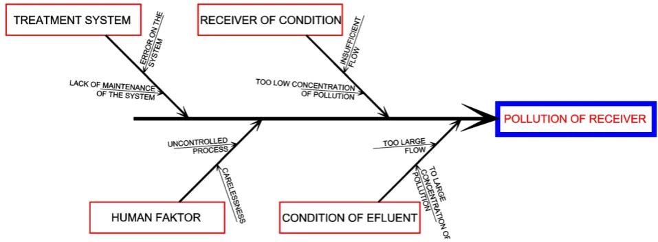
[image:2.595.318.550.449.632.2]

(3)

Figure 2. Ishikawa diagram of the system

Cause and Effect Analysis gives you a useful way of doing this. This diagram-based technique, which combines Brainstorming with a type of Mind Map, pushes you to consider all possible causes of a problem, rather than just the ones that are most obvious [7].

Although it was originally developed as a quality control tool, it can use the technique just as well in other ways. For instance, Ishikawa diagram can use it to:

• Discover the root cause of a problem. • Uncover bottlenecks in processes.

Ishikawa diagram shows causes of some effects. The diagram has a cause side (left) and the effect side (right). Exit or effect must be clearly defined. The result can be positive (target) or negative (a problem). Right from the central arrows draw the square - effect (pollution of river / receiver). It identifies the main causes that contribute to the effect. The main causes are divided on the treatment system, the human factor, the condition river (receiver) and effluent. For each main cause specific factors are identified. This is done by asking a series of questions “Why”.

3. The Mathematical Model

The mathematical model of real system was created, based on the system of differential-difference equations. The Runge-Kutta method was used to solve equation system.

Mathematical modelling framework was applied to develop the model component of receiver and effluent using differential and difference-differential equations. This occurs for the component according to the following reaction (1) written as differential equation. Concentrations are observed as changes in the concentration in the changing time, also flows too.

(2)

Whereas:

cds,1 – the initial value for downstream concentration of a

pollutant in receiver (river) (mg/l),

cus,1 – the initial value for upstream concentration of a

pollutant in receiver (river) (mg/l),

celv – emission limit value concentration of a pollutant in

river (mg/l),

Qus,1 – the initial value for upstream flow in receiver (river)

(m3_/s),

Qef – effluent flow (m3/s),

In the component, the difference equation was generated by using the Runge-Kutta method. Assuming that t(0) = 0, that is, at time t(0), the output cds(0) = 0, according to the

Runge-Kutta (IV) method, applies: cds(ti+1) = cdS(ti+Δti) =

= cdS(ti) + 1/6 [K1(i) + 2K2(i) + 2K3(i) + K4(i)] (3)

Whereas:

K1(i)= Δti· F(ti, cdS(ti)) (4)

K2(i)= Δti· F(ti+ Δti/2, cds(ti) + Δti/2 K1(i)) (5)

K3(i)= Δti· F(ti+ Δti/2, cdS(ti) + Δti/2 K2(i)) (6)

K4(i)= Δti· F(ti+ Δti/2, cdS(ti) + Δti K3(i)) (7)

4. The System Dynamics Model

System dynamics is an approach to understanding the nonlinear behaviour of complex systems over time using stocks and flows, internal feedback loops and time delays [10].

[image:3.595.63.542.87.263.2]

(4)

allow us to create management flight simulators-micro worlds where space and time can be compressed and slowed so we can experience the long-term side effects of decisions, speed learning, develop our understanding of complex systems, and design structures and strategies for greater success” [14].

The system dynamics model was created using the Powersim Constructor programme v. 2.51. (Figure 3). Flow diagram (the system dynamics model) provides detailed connection between the level, speed and delay. The system dynamics models, entities and events in the aggregate levels, which are actually the system state variables and flows. The levels leads to the accumulation of material while the flow of materials and information between the levels specified speed transition. The upstream concentration in receiver (river) (cus)

and upstream flow in receiver (river) (Qus) are used as a

random value from the theoretical probability distribution of real (empirical) values. Random number generators are marked blue. The parameters of the theoretical probability distribution of upstream concentration in receiver (river) are marked in red, and the parameters of the theoretical probability distribution of upstream flow in receiver (river) are marked in green in Figure 3. Emission limit value concentration of a pollutant in river (celv) and effluent flow

(Qef) are constants (marked in orange in Figure 3). In cds

(marked purple) is calculated by the system of equations with the method of Runge-Kutta (equations (3)-(7)).

Figure 3. System dynamics model

5. Results and Discussions

Empirical data from the flow of the river Bednja and concentration of pollutions in the river was obtained from the Croatian Meteorological Institute and Croatian Waters for a period of 5 years. Due to the limited research material, the samples were based on the total nitrogen. The monthly mean value of the data was calculated, while the Missing data belongs to Missing at Random (MAR)), the sample remains representative [1]. For the data processing the recommended deletion method is Listwise deletion, which is only used for the complete rows of table data [5, 3]. Values Missing at

Random (MAR) is an alternative to data Missing Completely at Random (MCAR), which occurs when the missing data is relating to a particular variable, for example an accidentally skipped answer from a questionnaire [10]. When one or more values are missing in a set of numbers, most software packages use Listwise Deletion Method. It is a simple method most commonly used for missing data management. This method deletes rows containing gaps, and uses only the complete ones [1, 5]. The interesting fact is that the Listwise Deletion Method, which is the simplest method, provides very good matching results with the probability distributions [3].

[image:4.595.311.553.319.593.2]

Using the applications Stat::Fit simulation packages Service Model Student Version, the characteristic theoretical distribution of the total nitrogen concentration and river flow, as well as the basic characteristics of descriptive statistics, was obtained. These data is shown in Table 1.

Table 1. Descriptive statistics and characteristic theoretical probability distribution of river flow and total nitrogen concentration

FLOW (m3_/s) CONCENTRATION (mg

N/l) Theoretical

distribution Lognormal (0; -0,34; 1,12) Lognormal (-1,21; 1,19; 0,458)

Data points 60 60

Minimum 0 0,13

Maximum 6,667 9,64

Mean 1,30022 2,45017

Median 0,6335 2,58

Mode 0,243 2,675

Standard deviation 1,52381 1,77556

Variance 2,322 3,1526

Coefficient of

variation 117,197 72,4667

Equation of Log – normal distribution (min, μ, σ) is:

f(x) = 1

(x−min)�2πσ2exp (−

[ln(x−min)− µ]2

2σ2 ) (8) whereas:

min – minimum x

μ – mean of the included Normal

σ – Standard deviation of the included Norma

The parameters of the log-normal distribution are entered into the system dynamics model. The value of emission limit value concentration of a pollutant in river (celv) is 2,6 mgN/L

(constant), and effluent flow (Qef) is 10 m3/s. The output

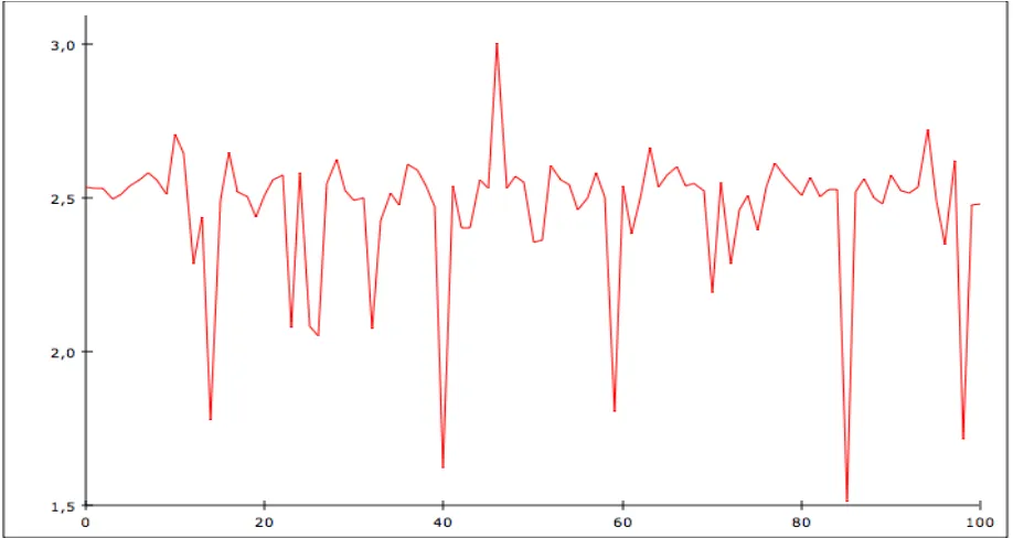
[image:4.595.62.290.416.532.2]

(5)

[image:5.595.75.534.79.323.2]

Figure 4. Downstream concentration of total nitrogen in receiver (river)

Downstream concentrations of total nitrogen in receiver (river) are variable in time. Depending on the upstream concentration and upstream flow rate can be regulated by the flow of the effluent.

The standard principle combined approach (equation (1) is using the mean or minimum value (worst case) to obtain a value without change in time. This approach often gives an incorrect and distorted view of the situation.

6. Conclusions

Based on the combined approach, a model that provides precise and a more accurate impact of effluent discharges into recipient (river) was developed. The focus of this paper is modelling the purifying systems for wastewater with acceptable work for effluent discharge into the recipient. In order to make the systems work in optimal conditions that are based on the concentrations of pollution data, receiver flow and effluent flow changes with time. The designing of a conceptual was required as well as a mathematical model. These models can show the reduction in the observed pollutants concentration, by using the systems of differential-difference equations for the purifiers considered, along with function equations for each substance.

Following the mathematical model functions work development, it was necessary to design a computer model as well. Mathematical functions present independent variables, while the water quality in the supplied water purification systems presents as a dependent variable. Searching the literature examples of using a combined approach was found. However, the main innovation and originality of this research is that the original equation of the combined approach is converted into the system of differential

equations and to observe changes in the concentration and flow depending on the time.

The input parameters were used according to the value of the total nitrogen concentrations from the effluent, river (upstream), and flow rate of the effluent and of the recipient. Moreover, the model is adaptable and can also be used for other concentrations and flow, or for studying the contamination of other substances. The methods of modelling and conceptualisation of such situations contribute significantly to environmental protection and human health.

In addition, the economic component of the system should also be taken into consideration. The developed adaptive model allows setting the optimal structure of the model according to the needs and working environment.

REFERENCES

[1] Allison P.D. Missing Data, Sage University Papers Series on Quantitative Applications in the Social Science, 2001.

[2] Gotal Dmitrović, L., Dušak, V., Anić Vučinić, A. The

Development of Conceptual, Mathematical and System Dynamics Model for Food Industry Wastewater Purifying System, JIOS, 39, pp.151-162, 2015

[3] Gotal Dmitrović, L., Dušak, V., Dobša, J. Missing data

problems in Non-Gaussian probability distributions, Informatologia, Vol. 49, 3- 4, 2016.

[4] Helo P.T. Dynamic modelling of surge effect and capacity limitation in supply chains; International Journal of Production Research; Volume 38, Number 17, 2000.,

(6)

Missing-Dana Methods for Generalised Linear Models: A Comparative Review, Journal of the American Statistical Association, 2005.

[6] Ishikawa, K. Guide to Quality Control, Asian Productivity Organization, UNIPUB. ISBN 92-833-1036-5, 1976. [7] Jackson, K. Cause and Effect Analysis - Identifying the Likely

Causes of Problems,https://www.mindtools.com/pages/articl e/newTMC_03.htm, downloaded: August, 18th 2015. [8] Kang, D., Choi, B. K. Visual Modelling and Simulation

Toolkit For Activity Cycle Diagram, http://www.scs-europe. net/conf/ecms2010/2010%20accepted%20papers/ibs_ECMS 2010_0037.pdf, downloaded: August, 18th 2015.

[9] Klingstram P. A methodology for supporting manufacturing system development; success factors for integrating simulation in the engineering process; New Supporting Tools for Designing Products and Production Systems, Leuven, 1999.,

[10]MIT System Dynamics in Education Project (SDEP), http://web.mit.edu/sysdyn/sd-intro/, downloaded: August, 18th 2015.

[11]Page, Jr., E. H. Simulation Modeling Methodology: Principles and Etiology of Decision Support, PhD thesis, Faculty of the Virginia Polytechnic Institute and State University, http://www.thesimguy.com/articles/simModMeth.pdf, downloaded: August, 17th 2015.

[12]Pidd M., Tools for Thinking – Modelling in Management Science; John Wiley & Sons New York; 1997.

[13]Shi, J. A Conceptual Activity Cycle-Based Simulation Modelling Method, http://www.informs-sim.org/wsc97paper s/1127.PDF, downloaded: August, 17th 2015.