Optimization of Manufacturing of Operational
Amplifier Manufactured
by
Using
Field-effect
Heterotransistor
to
Decrease Their Dimensions
E.
L. Pankratov
1,21
Nizhny Novgorod State University, Russia
2
Nizhny Novgorod State Technical University, Russia
Copyright©2019 by authors, all rights reserved. Authors agree that this article remains permanently open access under the terms of the Creative Commons Attribution License 4.0 International License
Abstract
In this paper we introduce an approach to decrease dimensions of operational amplifier based on field-effect heterotransistors. Dimensions of the elements will be decreased due to manufacture heterostructure with specific structure, doping of required areas of the heterostruc-ture by diffusion or ion implantation and optimization of annealing of dopant and/or radiation defects.Keywords
Operational Amplifier, Increasing Integration Rate of Field-effect Heterotransistors, Optimization of Manufacturing1. Introduction
In the present time density of elements of integrated circuits and their performance intensively increasing. Simultaneously with increasing of the density of these elements of integrated circuits their dimensions decreases. One way to decrease dimensions of these elements of these integrated circuit is manufacturing of these elements in thin-film heterostructures [1-4]. An alternative approach to
decrease dimensions of the elements of integrated circuits is using laser and microwave types annealing [5-7]. Using these types of annealing leads to generation inhomogeneous distribution of temperature. Due to Arrhenius law the inhomogeneity of the diffusion coefficient and other parameters of process. The inhomogeneity gives us possibility to decrease dimensions of elements of integrated circuits. Changing of properties of electronic materials could be obtain by using radiation processing of these materials [8,9].
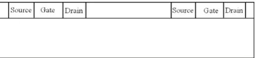
[image:1.595.171.429.597.741.2]In this paper we consider an operational amplifier based on field-effect heterotransistors described in Ref. [10] (see Fig.1). We assume, that the considered element has been manufactured in heterostructure from Fig. 1. The heterostructure consist of a substrate and an epitaxial layer. The epitaxial layer includes into itself several sections manufactured by using another materials. The sections have been doped by diffusion or ion implantation to generation into these sections required type of conductivity (n or p). In this paper we analyzed redistribution of dopant during annealing of dopant and/ or radiation defects to formulate conditions for decreasing of dimensions of the considered amplifier.
Figure 1b. Heterostructure with two layers and sections in the epitaxial layer
2. Method of solution
We determine spatio-temporal distribution of concentration of dopant by solving the following boundary problem
(1)
with boundary and initial conditions
, , , (2)
, , , C (x,y,z,0)=f (x,y,z).
Here C(x,y,z,t) is the spatio-temporal distribution of concentration of dopant; T is the temperature of annealing; DС is the dopant diffusion coefficient. Value of dopant diffusion coefficient depends on properties of materials, speed of heating and cooling of heterostructure (with account Arrhenius law). Dependences of dopant diffusion coefficients could be approximated by the following function [9,11,12]
, (3)
where DL (x,y,z,T) is the spatial (due to existing several layers wit different properties in heterostructure) and temperature (due to Arrhenius law) dependences of dopant diffusion coefficient; P(x,y,z,T) is the limit of solubility of dopant; parameter γ could be integer framework the following interval γ∈[1,3] [9]; V(x,y,z,t) is the spatio- temporal distribution of concentration of radiation vacancies; V* is the equilibrium distribution of concentration of vacancies. Concentrational dependence of dopant diffusion coefficient have been discussed in details in [9]. It should be noted, that using diffusion type of doping did not leads to generation radiation defects and ζ1= ζ2= 0. We determine spatio-temporal distributions of
concentrations of point defects have been determine by solving the following system of equations [11,12]
(4)
(
)
=
t
t
z
y
x
C
∂
∂
,
,
,
(
)
(
)
(
)
+
+
=
z
t
z
y
x
C
D
z
y
t
z
y
x
C
D
y
x
t
z
y
x
C
D
x
C C C∂
∂
∂
∂
∂
∂
∂
∂
∂
∂
∂
∂
,
,
,
,
,
,
,
,
,
(
)
0
,
,
,
0
=
∂
∂
=
x
x
t
z
y
x
C
(
)
0
,
,
,
=
∂
∂
=Lx x
x
t
z
y
x
C
(
)
0
,
,
,
0
=
∂
∂
=
y
y
t
z
y
x
C
(
)
0
,
,
,
=
∂
∂
=Ly x
y
t
z
y
x
C
(
)
0
,
,
,
0
=
∂
∂
=
z
z
t
z
y
x
C
(
)
0
,
,
,
=
∂
∂
=Lz x
z
t
z
y
x
C
(
)
(
(
)
)
(
)
(
( )
)
+
+
+
=
2* 2
2 *
1
,
,
,
,
,
,
1
,
,
,
,
,
,
1
,
,
,
V
t
z
y
x
V
V
t
z
y
x
V
T
z
y
x
P
t
z
y
x
C
T
z
y
x
D
D
C Lξ
γς
ς
γ
(
)
(
) (
)
(
) (
)
+
∂
∂
∂
∂
+
∂
∂
∂
∂
=
∂
∂
y
t
z
y
x
I
T
z
y
x
D
y
x
t
z
y
x
I
T
z
y
x
D
x
t
t
z
y
x
I
I I
,
,
,
,
,
,
,
,
,
,
,
,
,
,
,
(
) (
)
−
(
) (
) (
)
−
∂
∂
∂
∂
+
k
x
y
z
T
I
x
y
z
t
V
x
y
z
t
z
t
z
y
x
I
T
z
y
x
D
z
I IV,
,
,
,
,
,
,
,
,
,
,
,
,
,
,
,(
x
y
z
T
) (
I
x
y
z
t
)
k
I,I,
,
,
2,
,
,
[image:2.595.169.430.78.137.2]with boundary and i
nitial conditions
, , , ,
, , ρ(x,y,z,0)=fρ(x,y,z). (5)
Here ρ =I,V; I (x,y,z,t) is the spatio-temporal distribution of concentration of radiation interstitials; Dρ(x,y,z,T) is the diffusion coefficients of radiation interstitials and vacancies; terms V2(x,y,z,t) and I2(x,y,z,t) correspond to generation of divacancies and diinterstitials; kI,V(x,y,z,T) is the parameter of recombination of point radiation defects; kρ,ρ(x,y,z,T) are the
parameters of generation of simplest complexes of point radiation defects.
We determine spatio-temporal distributions of concentrations of divacancies ΦV(x,y,z,t) and diinterstitials ΦI(x,y,z,t) by solving the following system of equations [11,12]
(6)
with boundary and initial conditions
, , ,
, , , (7)
Φ
I(x,y,z,0)=f
ΦI(x,y,z), Φ
V(x,y,z,0)=f
ΦV(x,y,z).
(
)
(
) (
)
(
) (
)
+
∂
∂
∂
∂
+
∂
∂
∂
∂
=
∂
∂
y
t
z
y
x
V
T
z
y
x
D
y
x
t
z
y
x
V
T
z
y
x
D
x
t
t
z
y
x
V
V V,
,
,
,
,
,
,
,
,
,
,
,
,
,
,
(
) (
)
−
(
) (
) (
)
−
∂
∂
∂
∂
+
k
x
y
z
T
I
x
y
z
t
V
x
y
z
t
z
t
z
y
x
V
T
z
y
x
D
z
V IV,
,
,
,
,
,
,
,
,
,
,
,
,
,
,
,(
x
y
z
T
) (
V
x
y
z
t
)
k
V,V,
,
,
2,
,
,
−
(
)
0
,
,
,
0=
∂
∂
= xx
t
z
y
x
ρ
(
)
0
,
,
,
=
∂
∂
=Lx x
x
t
z
y
x
ρ
(
)
0
,
,
,
0=
∂
∂
= yy
t
z
y
x
ρ
(
)
0
,
,
,
=
∂
∂
=Ly y
y
t
z
y
x
ρ
(
)
0
,
,
,
0=
∂
∂
= zz
t
z
y
x
ρ
(
)
0
,
,
,
=
∂
∂
=Lz z
z
t
z
y
x
ρ
(
)
(
)
(
)
(
)
(
)
+
Φ
+
Φ
=
Φ
Φ Φy
t
z
y
x
T
z
y
x
D
y
x
t
z
y
x
T
z
y
x
D
x
t
t
z
y
x
I II I I
∂
∂
∂
∂
∂
∂
∂
∂
∂
∂
,
,
,
,
,
,
,
,
,
,
,
,
,
,
,
(
)
(
)
k
(
x
y
z
T
) (
I
x
y
z
t
) (
k
x
y
z
T
) (
I
x
y
z
t
)
z
t
z
y
x
T
z
y
x
D
z
I I II
I
,
,
,
,
,
,
,
,
,
,
,
,
,
,
,
,
,
,
+
, 2−
Φ
+
Φ∂
∂
∂
∂
(
)
(
)
(
)
(
)
(
)
+
Φ
+
Φ
=
Φ
Φ Φy
t
z
y
x
T
z
y
x
D
y
x
t
z
y
x
T
z
y
x
D
x
t
t
z
y
x
V VV V V
∂
∂
∂
∂
∂
∂
∂
∂
∂
∂
,
,
,
,
,
,
,
,
,
,
,
,
,
,
,
(
)
(
)
k
(
x
y
z
T
) (
V
x
y
z
t
)
k
(
x
y
z
T
) (
V
x
y
z
t
)
z
t
z
y
x
T
z
y
x
D
z
VV VV
V
,
,
,
,
,
,
,
,
,
,
,
,
,
,
,
,
,
,
+
, 2−
Φ
+
Φ∂
∂
∂
∂
(
)
0
,
,
,
0=
∂
Φ
∂
= xx
t
z
y
x
ρ
(
,
,
,
)
=
0
∂
Φ
∂
=Lx
x
x
t
z
y
x
ρ
(
)
0
,
,
,
0=
∂
Φ
∂
= yy
t
z
y
x
ρ(
)
0
,
,
,
=
∂
Φ
∂
=Ly y
y
t
z
y
x
ρ
(
)
0
,
,
,
0=
∂
Φ
∂
= zz
t
z
y
x
ρ
(
)
0
,
,
,
=
∂
Φ
∂
=Lz
Here DΦρ(x,y,z,T) are the diffusion coefficients of complexes of radiation defects; kρ(x,y,z,T) are the parameters of decay of complexes of radiation defects.
We determine spatio-temporal distributions of concentrations of dopant and radiation defects by using method of averaging of function corrections [13] with decreased quantity of iteration steps [14]. Framework the approach we used solutions of Eqs. (1), (4) and (6) in linear form and with averaged values of diffusion coefficients D0L, D0I, D0V, D0ΦI, D0ΦV as initial-order approximations of the required concentrations. The solutions could be written as
,
,
,
,
,
where , ,
cn(χ)=cos(πnχ/Lχ).
With the second-order approximations and higher orders approximations of concentrations of dopant and radiation defects we determine framework for standard iterative procedure [13,14]. Framework of this procedure to calculate approximations with the n-th-order one shall replace the functions C(x,y,z,t), I(x,y,z,t), V(x,y,z,t), ΦI(x,y,z,t), ΦV(x,y, z,t) in the right sides of the Eqs. (1), (4) and (6) on the following sums αnρ+ρn-1(x,y,z, t). As an example we present equations for
the second-order approximations of the considered concentrations
(8)
(
)
=
+
∑
∞( ) ( ) ( ) ( )
=1 0 12
,
,
,
n nC n n n nC
z y x z y x
C
F
c
x
c
y
c
z
e
t
L
L
L
L
L
L
F
t
z
y
x
C
(
)
=
+
∑
∞( ) ( ) ( ) ( )
=1 0 12
,
,
,
n nI n n n nI
z y x z y x
I
F
c
x
c
y
c
z
e
t
L
L
L
L
L
L
F
t
z
y
x
I
(
)
=
+
∑
∞( ) ( ) ( ) ( )
=1 0 12
,
,
,
n nC n n n nV
z y x z y x
C
F
c
x
c
y
c
z
e
t
L
L
L
L
L
L
F
t
z
y
x
V
(
)
=
+
∑
( ) ( ) ( )
( )
Φ
∞= Φ Φ
Φ 1 0 1
2
,
,
,
n n n n n n
z y x z y x
I
F
c
x
c
y
c
z
e
t
L
L
L
L
L
L
F
t
z
y
x
I I I(
)
=
+
∑
( ) ( ) ( )
( )
Φ
∞= Φ Φ
Φ 1 0 1
2
,
,
,
n n n n n n
z y x z y x
V
F
c
x
c
y
c
z
e
t
L
L
L
L
L
L
F
t
z
y
x
V V V( )
+
+
−
=
2 2 01
21
21
2exp
z y x nL
L
L
t
D
n
t
e
ρπ
ρ=
∫
( ) ( ) ( ) (
∫
∫
)
x y z
L L L
n n n
n
c
u
c
v
c
v
f
u
v
w
d
w
d
v
d
u
F
0 0 0
,
,
ρ ρ(
)
(
)
(
)
( )
[
(
(
)
)
]
×
+
+
+
+
=
∗ ∗T
z
y
x
P
t
z
y
x
C
V
t
z
y
x
V
V
t
z
y
x
V
x
t
t
z
y
x
C
C,
,
,
,
,
,
1
,
,
,
,
,
,
1
,
,
,
2 12 2 2 1 2 γ γ
α
ξ
ς
ς
∂
∂
∂
∂
(
)
(
)
(
)
(
)
(
)
( )
×
+
+
+
×
∗ ∗ 2 2 2 11
,
,
,
,
,
,
1
,
,
,
,
,
,
,
,
,
V
t
z
y
x
V
V
t
z
y
x
V
T
z
y
x
D
y
x
t
z
y
x
C
T
z
y
x
D
L Lς
ς
∂
∂
∂
∂
(
)
[
]
(
)
(
)
(
)
(
)
×
+
+
+
×
z
t
z
y
x
C
T
z
y
x
D
z
y
t
z
y
x
C
T
z
y
x
P
t
z
y
x
C
L C∂
∂
∂
∂
∂
∂
α
ξ
γ γ,
,
,
,
,
,
,
,
,
,
,
,
,
,
,
1
2 1 1 1(
)
(
)
( )
[
(
(
)
)
]
+
+
+
+
×
∗ ∗T
z
y
x
P
t
z
y
x
C
V
t
z
y
x
V
V
t
z
y
x
V
C,
,
,
,
,
,
1
,
,
,
,
,
,
1
2 1(
)
(
)
(
)
(
)
(
)
+
+
=
y
t
z
y
x
I
T
z
y
x
D
y
x
t
z
y
x
I
T
z
y
x
D
x
t
t
z
y
x
I
I I∂
∂
∂
∂
∂
∂
∂
∂
∂
∂
,
,
,
,
,
,
,
,
,
,
,
,
,
,
,
1 12
(
)
(
)
−
[
+
(
)
]
[
+
(
)
]
×
+
I
x
y
z
t
V
x
y
z
t
z
t
z
y
x
I
T
z
y
x
D
z
I I,
,
,
V,
,
,
,
,
,
,
,
,
1α
2 1α
2 1∂
∂
∂
∂
(
)
(
)
[
(
)
]
21 2 ,
,
x
,
y
,
z
,
T
k
x
,
y
,
z
,
T
I
x
,
y
,
z
,
t
k
I V−
I I I+
×
α
(9)
(
)
(
)
(
)
(
)
(
)
+
+
=
y
t
z
y
x
V
T
z
y
x
D
y
x
t
z
y
x
V
T
z
y
x
D
x
t
t
z
y
x
V
V V∂
∂
∂
∂
∂
∂
∂
∂
∂
∂
,
,
,
,
,
,
,
,
,
,
,
,
,
,
,
1 12
(
)
(
)
−
[
+
(
)
]
[
+
(
)
]
×
+
I
x
y
z
t
V
x
y
z
t
z
t
z
y
x
V
T
z
y
x
D
z
V I,
,
,
V,
,
,
,
,
,
,
,
,
1α
2 1α
2 1∂
∂
∂
∂
(
)
(
)
[
(
)
]
21 2 ,
,
x
,
y
,
z
,
T
k
x
,
y
,
z
,
T
V
x
,
y
,
z
,
t
k
IV−
V V V+
×
α
(
)
(
)
(
)
(
)
×
+
Φ
=
Φ
ΦΦ
D
x
y
z
T
y
x
t
z
y
x
T
z
y
x
D
x
t
t
z
y
x
I I II2
,
,
,
,
,
,
1,
,
,
,
,
,
∂
∂
∂
∂
∂
∂
∂
∂
(
)
(
)
(
)
+
(
)
×
Φ
+
Φ
×
Φk
x
y
z
T
z
t
z
y
x
T
z
y
x
D
z
y
t
z
y
x
I I I II
,
,
,
,
,
,
,
,
,
,
,
,
, 1 1∂
∂
∂
∂
∂
∂
(
x
y
z
t
)
k
(
x
y
z
T
) (
I
x
y
z
t
)
I
2,
,
,
−
I,
,
,
,
,
,
×
(
)
(
)
(
)
(
)
×
+
Φ
=
Φ
ΦΦ
D
x
y
z
T
y
x
t
z
y
x
T
z
y
x
D
x
t
t
z
y
x
V V VV2
,
,
,
,
,
,
1,
,
,
,
,
,
∂
∂
∂
∂
∂
∂
∂
∂
(10)(
)
(
)
(
)
+
(
)
×
Φ
+
Φ
×
Φk
x
y
z
T
z
t
z
y
x
T
z
y
x
D
z
y
t
z
y
x
V V V IV
,
,
,
,
,
,
,
,
,
,
,
,
, 1 1∂
∂
∂
∂
∂
∂
(
x
y
z
t
)
k
(
x
y
z
T
) (
V
x
y
z
t
)
V
2,
,
,
−
V,
,
,
,
,
,
×
Integration of the left and right sides of Eqs.(8)-(10) gives us possibility to obtain relations for the second-order approximations of concentrations of dopant and radiation defects in the final forms
(
)
(
)
(
)
( )
[
(
(
)
)
]
∫
×
+
+
+
+
=
∗ ∗ t CT
z
y
x
P
z
y
x
C
V
z
y
x
V
V
z
y
x
V
x
t
z
y
x
C
0 1 2 2 2 2 1 2,
,
,
,
,
,
1
,
,
,
,
,
,
1
,
,
,
γ γτ
α
ξ
τ
ς
τ
ς
∂
∂
(
)
(
)
(
)
(
)
( )
∫
×
+
+
+
×
∗ ∗ t LV
z
y
x
V
V
z
y
x
V
y
d
x
z
y
x
C
T
z
y
x
D
0 2 2 2 11
,
,
,
1
,
,
,
,
,
,
,
,
,
ς
τ
ς
τ
(8a) (9a) (10a)
(
)
[
(
(
)
)
]
(
)
(
)
∫
×
+
+
+
×
C t LL
D
x
y
z
T
z
d
y
z
y
x
C
T
z
y
x
P
z
y
x
C
T
z
y
x
D
0 1 12
,
,
,
,
,
,
,
,
,
,
,
,
1
,
,
,
∂
∂
τ
∂
τ
∂
τ
α
ξ
γ γ(
)
(
)
( )
[
(
(
)
)
]
(
)
+
+
+
+
+
×
∗∗
∂
τ
τ
∂
τ
α
ξ
τ
ς
τ
ς
γ γd
z
z
y
x
C
T
z
y
x
P
z
y
x
C
V
z
y
x
V
V
z
y
x
V
C,
,
,
,
,
,
,
,
,
1
,
,
,
,
,
,
1
2 1 12 2 2 1
(
x
y
z
)
f
C,
,
+
(
)
(
) (
)
+
∫
(
)
×
∫
=
t I tD
Ix
y
z
T
y
d
x
z
y
x
I
T
z
y
x
D
x
t
z
y
x
I
0 0 12
,
,
,
,
,
,
,
,
,
,
,
,
∂
∂
τ
∂
τ
∂
∂
∂
(
)
(
) (
)
(
)
×
∫
−
∫
+
×
t Id
tk
I Ix
y
z
T
z
z
y
x
I
T
z
y
x
D
z
d
y
z
y
x
I
0 , 0 11
,
,
,
,
,
,
,
,
,
τ
,
,
,
∂
τ
∂
∂
∂
τ
∂
τ
∂
(
)
[
+
]
+
(
)
−
∫
(
)
[
+
(
)
]
×
×
II
x
y
z
d
f
Ix
y
z
tk
IVx
y
z
T
II
x
y
z
0 1 2 , 2 1
2
,
,
,
τ
τ
,
,
,
,
,
α
,
,
,
τ
α
(
)
[
α
2V+
V
1x
,
y
,
z
,
τ
]
d
τ
×
(
)
(
)
(
)
+
∫
(
)
×
∫
=
t V tD
Vx
y
z
T
y
d
x
z
y
x
V
T
z
y
x
D
x
t
z
y
x
V
0 0 12
,
,
,
,
,
,
,
,
,
,
,
,
∂
∂
τ
∂
τ
∂
∂
∂
(
)
(
)
(
)
(
)
×
∫
−
∫
+
×
t Vd
tk
VVx
y
z
T
z
z
y
x
V
T
z
y
x
D
z
d
y
z
y
x
V
0 , 0 11
,
,
,
,
,
,
,
,
,
τ
,
,
,
∂
τ
∂
∂
∂
τ
∂
τ
∂
(
)
[
+
]
+
(
)
−
∫
(
)
[
+
(
)
]
×
×
IV
x
y
z
d
f
Vx
y
z
tk
IVx
y
z
T
II
x
y
z
0 1 2 , 2 1
2
,
,
,
τ
τ
,
,
,
,
,
α
,
,
,
τ
α
(
)
[
α
2V+
V
1x
,
y
,
z
,
τ
]
d
τ
×
(
)
(
)
(
)
+
∫
(
)
×
∫
Φ
=
Φ
t Φ I t ΦI
D
x
y
z
T
y
d
x
z
y
x
T
z
y
x
D
x
t
z
y
x
I I0 0
1
2
,
,
,
,
,
,
,
,
,
,
,
,
∂
∂
τ
∂
τ
∂
∂
∂
(
)
(
)
(
)
(
)
×
∫
+
∫
Φ
+
Φ
×
I t Φ Id
tk
I Ix
y
z
T
z
z
y
x
T
z
y
x
D
z
d
y
z
y
x
I 0 , 0 11
,
,
,
,
,
,
,
,
,
τ
,
,
,
∂
τ
∂
∂
∂
τ
∂
τ
∂
(
x
y
z
)
d
k
(
x
y
z
T
) (
I
x
y
z
)
d
f
(
x
y
z
)
I
I
t
I
,
,
,
,
,
,
,
,
,
,
,
0 2 Φ+
∫
−
×
τ
τ
τ
τ
(
)
(
)
(
)
+
∫
(
)
×
∫
Φ
=
Φ
t Φ V t ΦV
D
x
y
z
T
y
d
x
z
y
x
T
z
y
x
D
x
t
z
y
x
V V 0 0 12
,
,
,
We determine average values of the second-orders approximations of the considered concentrations by using the following standard relations [13,14]
. (11)
Substitution of relations (8a)-(10a) into relation (11) gives us possibility to obtain relations for the required average values α 2ρ
, (12)
(13a)
, (13b)
where ,
,
,
(
)
(
)
(
)
(
)
×
∫
+
∫
Φ
+
Φ
×
I t Φ Vd
tk
VVx
y
z
T
z
z
y
x
T
z
y
x
D
z
d
y
z
y
x
V
0 , 0
1
1
,
,
,
,
,
,
,
,
,
τ
,
,
,
∂
τ
∂
∂
∂
τ
∂
τ
∂
(
x
y
z
)
d
k
(
x
y
z
T
) (
V
x
y
z
)
d
f
(
x
y
z
)
V
V
t
V
,
,
,
,
,
,
,
,
,
,
,
0 2
Φ
+
∫
−
×
τ
τ
τ
τ
(
)
(
)
[
]
∫ ∫ ∫ ∫
−
Θ
=
Θ0 0 0 0
1 2
2
,
,
,
,
,
,
1
L L Lx y zz y x
t
d
x
d
y
d
z
d
t
z
y
x
t
z
y
x
L
L
L
ρ
ρ
α
ρ(
)
∫ ∫ ∫
=
L L Lx y zC z
y x
С
f
x
y
z
d
z
d
y
d
x
L
L
L
0 0 02
,
,
1
α
(
)
[
{
+
+
+
−
−
+
−
=
2 00 2 10 20 1100 2 10 01
00
2
1
4
2
1
IV II
IV V II IV
V II
IV II
I
A
A
A
A
A
A
A
A
α
α
α
(
)
00
00 2 10 01
2 1
0 0 0
2
1
,
,
1
II
IV V II
IV L L L
I z
y
x
A
A
A
A
x
d
y
d
z
d
z
y
x
f
L
L
L
x y z
+
+
+
α
−
∫ ∫ ∫
−
(
)
4 3 1
3 4
2 3 4 2
4
4
4
2
1
B
A
B
A
B
y
B
y
B
A
B
B
V+
−
+
−
−
+
=
α
(
)
(
) (
) (
)
∫
Θ
−
∫ ∫ ∫
Θ
=
Θ0 0 0 0
1 1
,
,
,
,
,
,
,
,
,
,
1
L L Lx y zj i
b a z
y x
abij
t
k
x
y
z
T
I
x
y
z
t
V
x
y
z
t
d
z
d
y
d
x
d
t
L
L
L
A
(
)
200 00 2
00 2
00 2
00
4
A
IVA
IV2
A
IVA
IIA
VVB
=
−
−
B
3=
A
IV00A
IV2 00+
A
IV01A
IV3 00+
A
IV00A
II10A
IV2 00−
(
−
)
[
+
(
+
+
)
−
(
+
+
)
]
−
−
4
A
IV2 00A
II00A
VV002
A
IV01A
IV002
A
IV001
A
IV01A
II102
A
II00A
IV10A
VV101
2 00 01 00 2
00 00
10
2
4
A
IVA
IIA
IV+
A
IVA
IVA
IV−
=
{
(
+
+
)
+
2+
00×
01 2
00 2
10 01
2 00
2
A
IV1
A
IVA
IIA
IVA
IVA
IVB
(
)
×
−
−
−
−
+
+
×
z y x II
IV II II
IV II
IV IV
IV IV
IV
L
L
L
A
A
A
A
A
A
A
A
A
A
A
4
4
1
2
00 00 00 01 00 10 10 00 00 11 20(
)
{
[
+
(
+
+
)
−
(
+
+
∫ ∫ ∫
×
,
,
2
01 002
001
01 102
00 101
0 0 0
IV II II
IV IV
IV IV L L L
I
![Figure 1a . Structure of the considered amplifier. View from top [10]](https://thumb-us.123doks.com/thumbv2/123dok_us/8788032.907936/1.595.171.429.597.741/figure-a-structure-considered-amplifier-view.webp)