Some Construction Methods of A Optimum Chemical Balance Weighing Designs

http://dx.doi.org/10.4236/jamp.2014.213136

How to cite this paper: Awad, R. and Banerjee, S. (2014) Some Construction Methods of A-Optimum Chemical Balance Weighing Designs. Journal of Applied Mathematics and Physics, 2, 1159-1170.

http://dx.doi.org/10.4236/jamp.2014.213136

Some Construction Methods of A-Optimum

Chemical Balance Weighing Designs

Rashmi Awad*_{, Shakti Banerjee}

School of Statistics, Devi Ahilya University, Indore, India Email: *_{awad.rashmi@gmail.com, shaktibn@yahoo.com}

Received 25September 2014; revised 26October 2014; accepted 3November 2014

Copyright © 2014 by authors and Scientific Research Publishing Inc.

This work is licensed under the Creative Commons Attribution International License (CC BY).

http://creativecommons.org/licenses/by/4.0/

Abstract

Some new construction methods of the optimum chemical balance weighing designs and pairwise efficiency and variance balanced designs are proposed, which are based on the incidence matrices of the known symmetric balanced incomplete block designs. Also the conditions under which the constructed chemical balance weighing designs become A-optimal are also been given.

Keywords

Balance Incomplete Block Design, Symmetric Balanced Incomplete Block Design, Variance

Balanced Design, Efficiency Balanced Design, Weighing Design, Chemical Balance Weighing Design, Optimum Chemical Balance Weighing Design, A-Optimal Chemical Balance Weighing Design

1. Introduction

Sir R. A. Fisher, a founder of modern concept of experimental designs gave the new ideas of designing in his first book Design of Experiment in the year 1935. Fisher’s work was continued by others; see [1]-[4]. The nec-essary and sufficient condition for a general block design to be variance balanced and efficiency balanced was given in the literature [5]-[8]. The concept of repeated blocks was introduced by Van Lint; see [9]. Further some potential applications of the balanced incomplete block designs with repeated blocks were presented in the lit-erature [10]-[13].

Another important concept which we discuss in this paper is weighing designs. The concept of weighing de-sign was originally given by Yates and formulated as a weighing problem by Hotelling and the condition of at-taining the lower bound by each of the variance of the estimated weights was given by him; see [14] [15]. In the latter developments, attention has been made in the direction of obtaining optimum weighing designs. Prominent work has been done by many researchers in this field; see [16]-[20]. In recent years, the new methods of con-structing the optimum chemical balance weighing designs and a lower bound for the variance of each of the es-*

timated weights from this chemical balance weighing design were obtained and a necessary and sufficient con-dition for this lower bound to be attained was proposed in the literature; see [21]-[24]. The constructions were based on the incidence matrices of balanced incomplete block designs, balanced bipartite block designs, ternary balanced block designs and group divisible designs.

Awad et al. [25] [26] gave the construction methods of obtaining optimum chemical balance weighing de-signs using the incidence matrices of symmetric balanced incomplete block dede-signs and some pairwise balanced designs were also been obtained which were efficiency as well as variance balanced. In that series we now pro-pose another new construction methods of obtaining optimum chemical balance weighing designs using the in-cidence matrices of symmetric balanced incomplete block designs and some more pairwise efficiency as well as variance balanced designs are proposed. Also we present the conditions under which the chemical balance weighing designs constructed by new construction methods leading to the A-optimal designs.

Let us consider ν treatments arranged in b blocks, such that the jth block contains kj experimental units and the ith treatment appears ri times in the entire design, i=1, 2,,ν ; j=1, 2,,b. For any block design there exist a incidence matrix N=   nij of order ν ×b, where nij denotes the number of experiment units in the jth block getting the ith treatment. When nij =1 or 0 ∀i and j, the design is said to be binary. Otherwise it is said to be nonbinary. In this paper we consider binary block designs only. The following addi-tional notations are used k=

[

k k1 2kb

]

′ is the column vector of block sizes, r=

[

r r1 2rv

]

′ is the column vector of treatment replication, Kb b× =diag

[

k k1 2kb

]

, Rv v× =diag

[

r r1 2rv

]

, Σ = Σ =ri kj n is the total num-ber of experimental units, with this N1b =r and N′ =1v k Where 1a is the a×1 vector of ones.

An equi-replicate, equi-block sized, incomplete design, which is also balanced in the sense given above is called balanced incomplete block design, which is an arrangement of ν symbols (treatments) into b sets (blocks) each containing k

(

k<ν

)

distinct symbols, such that any pair of distinct symbols occurs in exactly λ sets. Then it is easy to see that each treatment occurs in r

( )

>λ sets. ν, b, r, k, λ are called pa-rameters of the BIBD and the papa-rameters satisfies the relations ν =r bk, r k

(

− =1

)

λ ν

(

−1

)

and b≥ν

(Fisher’s Inequality). A BIB design is said to be symmetric if b=ν and r=k. In this case incidence matrix is a square matrix i.e. N′ =N. In case of symmetric balanced incomplete block design any two blocks have λ treatments in common.

Though there have been balanced designs in various senses (see [6] [27]). We will consider a balanced design of the following type.

A block design is called variance balanced if and only if

1) It permits the estimation of all normalized treatment contrasts with the same variance (see [7]). 2) If the information matrix for treatment effects C= −R NK N–1 ′ satisfies C=µ_I_ν −

( )

1ν 1 1_{ν ν}′_. where µ is the unique nonzero eigen value of the matrix C with the multiplicity

(

v−1

)

, I v is the v v× identity matrix.

A block design is called efficiency balanced if

1) Every contrast of treatment effects is estimated through the design with the same efficiency factor.

2) 1 1

( )

_{1 1}

(

( )

_{1 1}

)

o

M =R NK N− − ′− n _νr′=ψ I_ν n _νr′ ; see [2], and since M So =ψS, where ψ is the unique non zero eigen value of Mo with multiplicity

(

v−1

)

. For the EB block design N, the information matrix

C is given as C= −

(

1 ψ

)

(

R−

( )

1n rr′

)

; see [28].

A block design is said to be pairwise balanced if 1 b

ij i j j

n n′ =

= Λ

∑

(a constant) for all i, i′, i≠i′ and a pair- wise balanced block design is said to be binary if nij =0 or 1 only, for all i, j and it has parameters ν, b, r, k, Λ (=λ, say) [in this case, when r=r1v and k=k1b, it is a BIB design with parameters ν, b, r,

k, λ].

Weighing designs consists of n groupings of the p objects and suppose we want to determine the indi-vidual weights of p objects. We can fit the results into the general linear model

Y=X w e+ (1) where Y is an n×1 random column vector of the observed weights, w is the p×1 column vector repre- senting the unknown weights of objects and e is an n×1 random column vector of errors such that

( )

0_n

quanti-ties. The elements of matrix X take the values as

th th

th

th th

1 if the object is placed in the left pan in the weighing, 1 if the object is placed in the right pan in the weighing 0 if the object is not weighted in the weighing

th ij

j i

x j i

j i

+  = −_

 

The normal equations estimating w are of the form ˆ

X X w′ =X Y′ (2) where ˆw is the vector of the weights estimated by the least squares method.

The matrix X is called the design matrix. A weighing design is said to be singular or nonsingular, depend-ing on whether the matrix X X′ is singular or nonsingular, respectively. It is obvious that the matrix X X′ is nonsingular if and only if the matrix X is of full column rank

( )

= p . Now, if X is of full rank, that is, when

X X′ is nonsingular, the least squares estimate of w is given by

(

)

1

ˆ

w= X X′ − X Y′ (3) and the variance-covariance matrix of ˆw is

( )

_ˆ 2

(

)

1

Var w =σ X X′ − (4) When the objects are placed on two pans in a chemical balance, we shall call the weighings two pan weighing and the design is known as two pan design or chemical balance weighing design. In chemical balance weighing design, the elements of design matrix X =

( )

xij takes the values as +1 if the

th

j object is placed in the left pan in the ith weighing, −1 if the jth object is placed in the right pan in the ith weighing and 0 if the jth

object is not weighted in the ith weighing.

Hotelling has shown that if n weighing operations are to determine the weights of p=n objects, the minimum attainable variance for each of the estimated weights in this case is σ2 n and proved the theorem that each of the variance of the estimated weights attains the minimum if and only if X X′ =nIp (see [14]).

2. Variance Limit of Estimated Weights

Let X be an n×p matrix of rank p of a chemical balance weighing design and let mj be the number of times in which jth object is weighed, j=1, 2,,p (i.e. the mj be the number of elements equal to −1 and 1 in jth column of matrix X). Then Ceranka et al. (see [21]) proved the following theorem:

Theorem 2.1. For any n×p matrix X, of a nonsingular chemical balance weighing design, in which maximum number of elements equal to 1− and 1 in columns is equal to m, where m=max

{

m m₁, ₂,,m_p

}

. Then each of the variances of the estimated weights attains the minimum if and only if

p

X X′ =mI (5)

Also a nonsingular chemical balance weighing design is said to be optimal for the estimating individual weights of objects if the variances of their estimators attain the lower bound given by,

( )

ˆ 2

Var w , j 1, 2, ,p m

σ

= = _ (6)

In SBIB design D v r

(

, ,λ

)

; the block intersection between any two blocks is constant i.e. λ. Using this concept Banerjee (see [29]) proved the following results;

Proposition 2.2. Existence of SBIB design 

(

v r, ,λ

)

; implies the existence of a BIB design ′ with pa-

rameters v′ =v, 2 2

v b′ = _{ }

 , r′ =r

(

ν−1

)

, k′ =k, 2 2

k

λ′ = _{ }  .

Proposition 2.3. Existence of SBIB design 

(

v r, ,λ

)

; implies the existence of a BIB design ′ with pa-

rameters v′ =v,

2

v b′ =λ_{ }

 , 2

r r′ =r_{ }

 , k′ =k, 2

k

λ′ =λ_{ }  .

3. Construction of Design Matrix: Method I

In SBIB design D with the parameters v=b, r=k, λ; fix the th

to the j th fixed block, give negative sign to all the λ common treatments of remaining

(

b−1

)

blocks. Then eliminate that fixed block. Thus matrix N1 of design D1 is obtained.

Now doing the same procedure for all the remaining

(

b−1

)

blocks, the incidence matrix N∗1 of the new design D∗1 so formed is the matrix having the elements 1, −1 and 0; given as follows

[

]

1 1 2

N∗ = N N N_ν (7)

Then combining the incidence matrix N of SBIB design repeated s-times with N∗1 we get the matrix X

of a chemical balance weighing design as

-times

1 s

X N∗ N N

′

 

 

=

 

 



  (8)

Under the present construction scheme, we have 2

2 b

v n  _{ }+s

 

= and p=v. Thus the each column of X

will contain ρ1=r b r

(

− +

)

srelements equal to 1, ρ2=r r

(

−1

)

elements equal to −1 and n−ρ ρ1− 2 ele-ments equal to zero. Clearly such a design implies that each object is weighted m=ρ ρ1+ 2=r b

(

− +1

)

sr

times in 2

2 b

v n  _{ }+s

 

= weighing operations.

Lemma 3.1. A design given by X of the form (8) is non singular if and only if r b r

(

−

) (

≠ λ−k

)(

4λ+s

)

.

Proof. For the design matrix X given by (8), we have

(

)

{

}

{

(

)

(

)

}

{

(

)

(

)

}

(

) (

)(

)

{

}

{

(

)

(

(

)

)

}

1 1 4 1 4

4 1 4

X X r sr k k k s I k k k s J

X X r b r k s I k k k s J

ν νν

ν νν

ν λ λ λ λ λ λ

λ λ λ λ

 

′ =_ − + − − − − + _ + − − − +

 

′

⇒ =_ − + − + _ + − − − − (9)

and

(

) (

) (

{

)

(

(

)

)

}

(

)

{

(

)

(

(

)

)

}

1

1 1 1 4 1 1 4

X X′ =_r b− + +s ν− k k− −λ k−λ −s  _{ }× r b− + −s k k− −λ k−λ −s _ν− (10)

the determinant (10) is equal to zero if and only if

(

1

)

(

1

)

(

4

(

)

)

(

) (

)(

4

)

r b− +s =k k− −λ k−λ − ⇒s r b−r = λ−k λ+s

or r b

(

− + = −1 s

) (

1 ν

) (

{

k k− −1

)

λ

(

4

(

k−λ

)

−s

)

}

but r b

(

− + +1 s

) (

ν−1

) (

{

k k− −1

)

λ

(

4

(

k−λ

)

−s

)

}

is positive and then det

(

X X′ =

)

0 if and only if

(

) (

)(

4

)

r b r− = λ−k λ+s . So the lemma is proved. □

Theorem 3.2. The non-singular chemical balance weighing design with matrix X given by (8) is optimal if and only if

(

1

)

4

(

)

k k− =λ_ k−λ −s_ (11)

Proof. From the conditions (5) and (9) it follows that a chemical balance weighing design is optimal if and only if the condition (11) holds. Hence the theorem.

If the chemical balance weighing design given by matrix X of the form (8) is optimal then

( )

₍

2

₎

ˆ

Var ; 1, 2, ,

1 j

w j p

r b s

σ

= =

− + 

Example 3.3. Consider a SBIB design with parameters v= =b 7, r= =k 4, λ =2; whose blocks are gi- ven by (3,5,6,7), (1,4,6,7), (1,2,5,7), (1,2,3,6), (2,3,4,7), (1,3,4,5), (2,4,5,6).

1 0 0 1 0 1 1

1 1 0 0 1 0 1

1 1 1 0 0 1 0

0 1 1 1 0 0 1

1 0 1 1 1 0 0

0 1 0 1 1 1 0

0 0 1 0 1 1 1

1 1 0 0 1 0 1

1 1 1 0 0 1 0

0 1 1 1 0 0 1

1 0 1 1 1 0 0

0 1 0 1 1 1 0

0 0 1 0 1 1 1

1 0 0 1 0 1 1

1 1 1 0 0 1 0

0 1 1 1 0 0 1

1 0 1 1 1 0 0

0 1 0 1 1 1 0

0 0 1 0 1 1 1

1 0 0 1 0 1 1

1 1 0 0 1 0 1

0 1 1 1 0 0 1

1 − − − − − − − − − − − − − − − − − − − − − − − − − − − − − − − − − − − − − − − − − − − −

− 0 1 1 1 0 0

0 1 0 1 1 1 0

0 0 1 0 1 1 1

1 0 0 1 0 1 1

1 1 0 0 1 0 1

                                                                     ₋     _{− −}    − −    _{− −}   − −    

1 1 1 0 0 1 0

1 0 1 1 1 0 0

0 1 0 1 1 1 0

0 0 1 0 1 1 1

1 0 0 1 0 1 1

1 1 0 0 1 0 1

1 1 1 0 0 1 0

0 1 1 1 0 0 1

0 1 0 1 1 1 0

0 0 1 0 1 1 1

1 0 0 1 0 1 1

1 1 0 0 1 0 1

1 1 1 0 0 1 0

0 1 1 1 0 0 1

1 0 1 1 1 0 0

0 0 1 0 1 1 1

1 0 0 1 0 1 1

1 1 0 0 1 0 1

1 1 1 0 0 1 0

0 1 1 1 0 0 1

1 0 1 1 1 0 0

0 1 0 1 1 1 0

- --− − − − − − − − − − − − − − − − − − − − − − − − − − − − − −             

0 0 1 0 1 1 1

1 0 0 1 0 1 1

1 1 0 0 1 0 1

1 1 1 0 0 1 0

0 1 1 1 0 0 1

1 0 1 1 1 0 0

0 1 0 1 1 1 0

Clearly such a design implies that each object is weighted m=32 times in n=56 weighing operations and

( )

_ˆ 2

Var w_j =σ 32 for each j=1, 2,, 7.

Corollary 3.4. If the SBIB design exists with parameters ν = =b N, r= =k

(

N±d

)

2, λ=

(

N±2d+1 4

)

; then the design matrix N∗1 so formed using above method is optimum chemical balance weighing design.

Corollary 3.5. If in the design D∗1; −1 is replaced by zero then the new design D∗∗1 so formed is a BIB

design with parameters V =ν, 2 2

B= _{ }v

 , R=r b r

(

−

)

, K = −k λ, 2 2

k−λ



Λ = _ _

 . Then the structure

-times 1

1 s

N∗ N_∗∗ N N

 

 

=

 

 



  (12)

form a pairwise VB and EB design D*1 with parameters 1

V

ν∗ ₌

, b∗1 = +B sb, r∗2= +R sr,

1 1 1

1 , 2 , ,

k∗ = −k λ k∗ =k λ∗ = Λ +sλ

(

)

(

)

1 1

1

1 s and 1 1 s .

k k

k r k

λ ν λ

µ∗ ν λ ψ∗ λ

∗

   

= _ − − + _ = − _ − − + _

   

4. Construction of Design Matrix: Method II

In SBIB design D with the parameters ν =b, r=k, λ; consider the λ blocks containing any pair of treatments say

(

θ ψ,

)

. Now rearranging the λ-blocks corresponding to the pair

(

θ ψ,

)

and giving the nega-tive sign to the treatments θ and ψ both; the matrix N1 of design D1 is obtained.

Now doing the same procedure for all the 2

v

   

  sets of blocks, the incidence matrix N∗2 of the new design

2

D∗ so formed is the matrix having the elements 1, −1 and 0; given as follows

2 1 2

2

N_∗ N N N_{ ν}    

 

 

=

 

   

(13)

Then combining the incidence matrix N of SBIB design repeated s-times with N∗2 we get the matrix

X of a chemical balance weighing design as

-times

2 s

X N∗ N N

′

 

 

=

 

 



  (14)

Under the present construction scheme, we have

2

v sb n λ _{ }+

 

= and p=v. Thus the each column of X

will contain 1 3 3

r sr

ρ =  _{ }+

  elements equal to 1, ρ2 =r k

(

−1

)

elements equal to 1− and n–ρ ρ1– 2

ele-ments equal to zero. Clearly such a design implies that each object is weighted 1 2 2

k m ρ ρ r  +sr

 

= + = times

in

2

v sb n λ _{ }+

 

= weighing operations.

Lemma 4.1. A design given by X of the form (14) is non singular if and only if λ 2_νr−

(

k−4

)

2_≠s

(

λ−r

)

.

(

)

(

)

(

)

(

)

2 2 2 2 4 2 2 4 2

4 ( )

2

4 2

k

r sr k k s I

k k s

X X

X

J

r k s r I

k k s J

X ν νν ν νν λ _λ λ _λ

λ ν λ

λ _λ      _{ }  =_{  }+ _{ }− _ − − _+ _           _{ }  +_{ } − − _+ _    _{ }  ⇒ =_{ } − − _+ − _    _{ }  +_{ } − − _+ _   ′ ′ (15) and

(

)

(

)

(

)

2 1 2 1 4 2 2 4 2 2 k

r sr k k s

r

r sr k k

X X

s

ν

λ

ν λ

λ _λ −

     _{ }  =  + + −  _ − − _+                  _{ }  ×  +  − _ − − _+             ′ (16)

the determinant (16) is equal to zero if and only if

(

)

(

)

(

)

2 2 2 4 2 4 2 k r sr

k k s

r k s r λ _λ λ ν λ  ₊       = _ − − _+   ⇒ _ − − _ = −

or

(

1

)

(

4

)

2

2 2

k

r  +sr= −ν λ_ k− −k_+sλ

 

 

but

(

1

)

(

4

)

2

2 2

k

r sr ν λ k k sλ

   

 ₊ _{+ −}  _{ − − +} 

     _{ } 

 

   

  is positive and then det

(

X X′ =

)

0 if and only if

(

)

2

(

)

2 r k 4 s r

λ _ν − − _= λ− . So the lemma is proved. □

Theorem 4.2. The non-singular chemical balance weighing design with matrix X given by (8) is optimal if and only if

(

)

2

[

]

4 2

k− = k− s (17)

Proof. From the conditions (5) and (15) it follows that a chemical balance weighing design is optimal if and only if the condition (17) holds. Hence the theorem.

If the chemical balance weighing design given by matrix X of the form (14) is optimal then

( )

2 ˆ

Var ; 1, 2, ,

2 j

w j p

k r s σ = =    +        

Example 4.3. Consider a SBIB design with parameters v= =b 7, r= =k 3, λ =1; whose blocks are given by (1,2,4), (2,3,5), (3,4,6), (4,5,7), (1,5,6), (2,6,7), (1,3,7).

1 1 0 1 0 0 0

1 0 1 0 0 0 1

1 1 0 1 0 0 0

1 0 0 0 1 1 0

1 0 0 0 1 1 0

1 0 1 0 0 0 1

0 1 1 0 1 0 0

1 1 0 1 0 0 0

0 1 1 0 1 0 0

0 1 0 0 0 1 1

0 1 0 0 0 1 1

0 0 1 1 0 1 0

0 1 1 0 1 0 0

0 0 1 1 0 1 0

1 0 1 0 0 0 1

0 0 0 1 1 0 1

0 0 1 1 0 1 0

0 0 0 1 1 0 1

1 0 0 0 1 1 0

0 0 0 1 1 0 1

0 1 0 0 0 1 1

1 1

X

− −

− −

− −

− −

− −

− −

− −

− −

− −

− −

− −

− −

− −

− −

= − −

− −

− −

− −

− −

− −

− −

      

0 1 0 0 0

0 1 1 0 1 0 0

0 0 1 1 0 1 0

0 0 0 1 1 0 1

1 0 0 0 1 1 0

0 1 0 0 0 1 1

1 0 1 0 0 0 1

 

 

 

 

 

 

 

 

 

 

 

 

 

 

 

 

 

 

 

 

 

 

 

 

 

 

 

 

 

 

 

 

 

 

 

 

 

 

 

 

 

 

 

 

 

 

Clearly such a design implies that each object is weighted m=12 times in n=28 weighing operations and

( )

_ˆ 2

Var w_j =σ 12 for each j=1, 2,, 7.

Corollary 4.4. If the SBIB design exists with block size r≤6 and λ ≤5; then the design matrix X so formed using above method II is optimum chemical balance weighing design.

Corollary 4.5. If the SBIB design exists with parameters

(

ν ν, −1,ν−2

)

; then the design matrix X given by (14) is optimum chemical balance weighing design if and only if v≤7.

Corollary 4.6. If in the design D∗2; −1 is replaced by zero then the new design D∗∗2 so formed is a BIB

design with parameters V =ν,

2

B=λ v

 , R 3 3

r



= _{ }

 , K= −k 2, Λ =λ 2

(

k−2

)(

k−3

)

. Then the struc-ture

-times

2 2

s

N∗ N_∗∗ N N

 

 

=

 

 



  (18)

2 V

ν∗ ₌

, b∗2 = +B sb, r∗2= +R sr, k12 k 2

∗ _{= −}

, k22 k

∗ ₌

, λ∗2= Λ +sλ,

(

)

(

)

2 2

2

3 3

and 1

2 2

k s k s

k r k

νλ

µ∗ νλ ψ∗

∗

− −

   

= _ + _ = − _ + _

   

5. A-Optimality of Chemical Balance Weighing Design

Some problems related to the optimality of chemical balance weighing designs were considered in the literature; see [17] [30] [31]. Wong and Masaro [32] [33] gave the lower bound for tr_

(

X X′

)

−1_ and some construction methods of the A-optimal chemical balance weighing designs.

Let X be a n×p design matrix of a chemical balance weighing design. Then the following results from Ceranka et al. [34] give the lower bound for tr_

(

X X′

)

−1_.

Theorem 5.1. For any nonsingular chemical balance weighing design with the design matrix X =

( )

xij we

have

(

)

1 2

tr X X p

q n

−

 _′ _≥

  _⋅ (19)

where q=max

(

q q1, 2,,qn

)

,

2 1 j p

ij i

q =

∑

₌ x , i=1, 2,,n.

The case when q= p; we get the inequality given in Wong and Masaro [32].

Definition 5.2. Any nonsingular chemical balance weighing design with the design matrix X =

( )

xij is said

to be A-optimal if

(

)

1 2

tr X X p

q n

−

 ′ =

  _⋅ (20)

Theorem 5.3. Any nonsingular chemical balance weighing design with the design matrix X =

( )

x_ij is A-optimal if and only if

p

q n

X X I

p

⋅

′ = (21)

6. Checking the A-Optimality in Methods I and II

For the construction Method I of chemical balance weighing design; the Lemma 3.1 proven above gave the nec-essary condition for the design matrix X of the form (8) to be non-singular.

Theorem 6.1. The non-singular chemical balance weighing design with matrix X given by (8) is A-optimal if and only if

(

1

)

4

(

)

k k− =λ_ k−λ −s_ (22)

(

) (

)(

)

(

)

and r b r k 4 q v 1 sb

v

s v

λ λ

− + − + =  − +  (23)

Proof. For the design matrix X given in (8) we have

(

)

{

}

{

(

)

(

)

}

{

(

)

(

)

}

(

) (

)(

)

{

}

(

)

{

(

)

}

1 1 4 1 4

4 1 4

X X r sr k k k s I k k k s J

X X r b r k s I k k k s J

ν νν

ν νν

ν λ λ λ λ λ λ

λ λ λ λ

 

′ =_ − + − − − − + _ + − − − +

   

′

⇒ =_ − + − + _ +_ − − − − _

and

(

1

)

v

q v v

X b

v

X′ =  − +s I

(

1

)

4

(

)

k k− =λ_ k−λ −s_

and

(

1

)

{

(

1

)

4

(

)

}

q

(

1

)

(

) (

)(

4

)

(

1

)

r sr k k k s v v sb r b r k s q v v sb

v v

ν− + − − − λ −λ + λ =  − + ⇒ − + −λ λ+ =  − + 

If (22) is satisfied then we get the condition (23) from the last equation. Hence the theorem.

For the construction Method II of chemical balance weighing design; the Lemma 4.1 proven above gave the necessary condition for the design matrix X of the form (14) to be non-singular.

Theorem 6.2. The non-singular chemical balance weighing design with matrix X given by (14) is A-op- timal if and only if

(

) (

2

)

4 2

k− = k− s (24) and

(

)

2

(

)

2 4

2

q sb

r k s r

v

ν λ

λ ν λ

  ₊ 

   

 

 

 _{− −} _{+ − =}

  (25)

Proof. For the design matrix X given in (14) we have

(

)

(

)

(

)

(

)

(

)

2 2

2 2

4 4

2 2 2

4 4

2 2

k

r sr k k s I k k s J

r k s r I k k s J

X X

X X

ν νν

ν νν

λ _λ λ _λ

λ _{ν λ} λ _λ

     _{ }   _{ } 

=_{  }+ _{ }− _ − − _+ _ +_{ } − − _+ _

   

    

 

 

 _{ }  _{ }

⇒ =_{ } − − _+ − _ +_{ } − − _+ _

 

 

′

′

and

2

q sb

I v

X X ν

ν λ

   

+

   

 

′ =  

Comparing these two equalities we get

(

) (

2

)

4 2

k− = k− s

and

(

)

2 2

(

)

2

(

)

2

4 4

2 2 2

q sb q sb

k

r sr k k s r k s r

v v

ν ν

λ λ

λ _λ λ _{ν λ}

       

+ +

       

   

 ₊  _{−  − − +} ₌    _{⇒  − − + − =}    

     _{ }  _{ }

 

   

 

If (24) is satisfied then we get the condition (25) from the last equation. Hence the theorem.

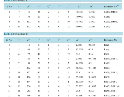
7. Discussion

The following Table 1and Table 2 provide the list of pairwise variance and efficiency balanced block designs for Methods I and II respectively, which can be obtained by using certain known SBIB designs.

8. Conclusion

[image:11.595.79.510.89.425.2]

Table 1. For method I.

S. No. ν∗1 1

b∗ _r∗1 1

1

k∗ 1

2

k∗ λ∗1 µ∗1 ψ∗1

Reference No.**

1 7 56 18 2 3 4 11.6667 0.3519 R (10), MH (1)

2 7 56 20 2 4 6 14.0000 0.3000 R (11)

3 11 132 40 3 5 10 30.8000 0.2300 R (29), MH (5)

[image:11.595.83.510.93.430.2]

4 11 132 42 3 6 12 33.0000 0.2143 R (30)

Table 2.For method II.

S. No. ν∗2 2

b∗ 2

r∗ k12

∗ 2

2

k∗ λ∗2 µ∗2 ψ∗2

Reference No.**

1 4 16 6 1 3 0 2.6667 0.5556 R (2)

2 5 40 20 2 4 3 15.0000 0.25 R (4)

3 6 72 40 3 5 12 33.6 0.16 R (8)

4 7 28 6 1 3 0 2.3333 0.61111 R (10), MH (1)

5 7 56 20 2 4 2 14.0000 0.3 R (11)

6 7 112 66 4 6 30 58.3333 0.11616 R (13)

7 11 132 40 3 5 6 30.8 0.23 R (29), MH (5)

8 11 176 66 4 6 18 55.0000 0.16667 R (30)

9 13 104 20 2 4 1 13.0000 0.35 R (37), MH (3)

10 16 256 66 4 6 12 53.3333 0.19192 R (47), MH (10)

11 21 252 40 3 5 3 29.4 0.265 R (58), MH (7)

12 31 496 66 4 6 6 51.6667 0.21717 R (75), MH (12)

**_{The symbols R}( )_{α and MH}( )_{α denote the reference number α in Raghavrao [30] and Marshal Halls [35] list.}

the constructed chemical balance weighing designs lead to A-optimal designs. The only limitation of this re-search is that the obtained pairwise balanced designs all have large number of replications.

Acknowledgments

We are grateful to the anonymous referees for their constructive comments and valuable suggestions.

References

[1] Agrawal, H.L. and Prasad, J. (1982) Some Methods of Construction of Balanced Incomplete Block Designs with Nested Rows and Columns. Biometrika, 69, 481-483. http://dx.doi.org/10.1093/biomet/69.2.481

[2] Caliski, T. (1971) On Some Desirable Patterns in Block Designs. Biometrika, 27, 275-292.

http://dx.doi.org/10.2307/2528995

[3] Hanani, H. (1975) Balanced Incomplete Block Designs and Related Designs. Discrete Mathematics, 11, 255-269.

http://dx.doi.org/10.1016/0012-365X(75)90040-0

[4] Shrikhande, S.S. and Raghavarao, D. (1963) A Method of Construction of Incomplete Block Designs. Sankhya, A25, 399-402.

[5] Jones, R.M. (1959) On a Property of Incomplete Blocks. Journal of the Royal Statistical Society, B21, 172-179.

[6] Puri, P.D. and Nigam, A.K. (1975) On Patterns of Efficiency Balanced Designs. Journal of the Royal Statistical Soci-ety, B37, 457-458.

[7] Rao, V.R. (1958) A Note on Balanced Designs. Annals of the Institute of Statistical Mathematics, 29, 290-294.

http://dx.doi.org/10.1214/aoms/1177706729

[9] Van Lint, J.H. (1973) Block Designs with Repeated Blocks and (b; r; λ) = 1. Journal of Combinatorics Theory, A15, 88-309.

[10] Ceranka, B. and Graczyk, M. (2007) Variance Balanced Block Designs with Repeated Blocks. Applied Mathematical

Sciences, 1, 2727-2734.

[11] Ceranka, B. and Graczyk, M. (2009) Some Notes about Efficiency Balanced Block Designs with Repeated Blocks.

Metodoloski Zvezki, 6, 69-76.

[12] Ghosh, D.K. and Shrivastava, S.B. (2001) A Class of Balanced Incomplete Block Designs with Repeated Blocks.

Journal of Applied Statistics, 28, 821-833. http://dx.doi.org/10.1080/02664760120074915

[13] Hedayat, A. and Federer, W.T. (1972) Pairwise and Variance Balanced Incomplete Block Designs. Annals of the

Insti-tute of Statistical Mathematics, 26, 331-338. http://dx.doi.org/10.1007/BF02479828

[14] Hotelling, H. (1944) Some Improvements in Weighing and Other Experimental Techniques. Annals of Mathematical

Statistics, 15, 297-306. http://dx.doi.org/10.1214/aoms/1177731236

[15] Yates, F. (1935) Complex Experiments. Supplement to the Journal of the Royal Statistical Society, 2, 181-247.

[16] Banerjee, K.S. (1948) Weighing Designs and Balanced Incomplete Blocks. Annals of Mathematical Statistics, 19, 394-399. http://dx.doi.org/10.1214/aoms/1177730204

[17] Banerjee, K.S. (1975) Weighing Designs for Chemistry, Medicine, Economics, Operations Research, Statistics. Marcel Dekker Inc., New York.

[18] Dey, A. (1969) A Note on Weighing Designs. Annals of the Institute of Statistical Mathematics, 21, 343-346.

http://dx.doi.org/10.1007/BF02532262

[19] Dey, A. (1971) On Some Chemical Balance Weighing Designs. Australian Journal of Statistics, 13, 137-141.

http://dx.doi.org/10.1111/j.1467-842X.1971.tb01252.x

[20] Raghavarao, D. (1959) Some Optimum Weighing Designs. Annals of Mathematical Statistics, 30, 295-303.

http://dx.doi.org/10.1214/aoms/1177706253

[21] Ceranka, B. and Graczyk, M. (2001) Optimum Chemical Balance Weighing Designs under the Restriction on the Number in Which Each Object Is Weighed. Discussiones Mathematicae: Probability and Statistics, 21, 113-120.

[22] Ceranka, B. and Graczyk, M. (2002) Optimum Chemical Balance Weighing Designs Based on Balanced Incomplete Block Designs and Balanced Bipartite Block Designs. Mathematica, 11, 19-27.

[23] Ceranka, B. and Graczyk, M. (2004) Ternary Balanced Block Designs Leading to Chemical Balance Weighing De-signs for v + 1 Objects. Biometrica, 34, 49-62.

[24] Ceranka, B. and Graczyk, M. (2010) Some Construction of Optimum Chemical Balance Weighing Designs. Acta

Uni-versitatis Lodziensis, Folia Economic, 235, 235-239.

[25] Awad, R. and Banerjee, S. (2013) Some Construction Methods of Optimum Chemical Balance Weighing Designs I.

Journal of Emerging Trends in Engineering and Applied Sciences (JETEAS), 4, 778-783.

[26] Awad, R. and Banerjee, S. (2014) Some Construction Methods of Optimum Chemical Balance Weighing Designs II.

Journal of Emerging Trends in Engineering and Applied Sciences (JETEAS), 5, 39-44.

[27] Caliski, T. (1977) On the Notation of Balance Block Designs. In: Recent Developments in Statistics, North-Holland Publishing Company, Amsterdam, 365-374.

[28] Kageyama, S. (1974) On Properties of Efficiency Balanced Designs. Communications in Statistics-Theory and Meth-ods, 9, 597-616.

[29] Banerjee, S. (1985) Some Combinatorial Problems in Incomplete Block Designs. Unpublished Ph.D. Thesis, Devi Ahilya University, Indore.

[30] Raghavarao, D. (1971) Constructions and Combinatorial Problems in Designs of Experiments. John Wiley, New York.

[31] Shah, K.R. and Sinha, B.K. (1989) Theory of Optimal Designs. Springer-Verlag, Berlin, Heidelberg.

http://dx.doi.org/10.1007/978-1-4612-3662-7

[32] Wong, C.S. and Masaro, J.C. (1984) A-Optimal Design Matrices X

( )

x_{ij N n}

×

= with x_ij= −1, 0, 1. Linear and

Mul-tilinear Algebra, 15, 23-46. http://dx.doi.org/10.1080/03081088408817576

[33] Jacroux, M., Wong, C.S. and Masaro, J.C. (1983) On the Optimality of Chemical Balance Weighing Designs. Journal

of Statistical Planning and Inference, 8, 231-240. http://dx.doi.org/10.1016/0378-3758(83)90041-1

[34] Ceranka, B. and Graczyk, M. (2007) A-Optimal Chemical Balance Weighing Design under Certain Conditions.

Me-todoloski Zvezki, 4, 1-7.