A Semi Implicit Scheme of Lattice Boltzmann Method for Two Dimensional Cavity Flow Simulation

http://dx.doi.org/10.4236/ojfd.2015.51002

How to cite this paper: Zhang, L., Yao, J., Sun, H. and Zhang, J.G. (2015) A Semi-Implicit Scheme of Lattice Boltzmann Me-thod for Two Dimensional Cavity Flow Simulation. Open Journal of Fluid Dynamics, 5, 10-16.

http://dx.doi.org/10.4236/ojfd.2015.51002

A Semi-Implicit Scheme of Lattice

Boltzmann Method for Two

Dimensional Cavity Flow Simulation

Lei Zhang

1

, Jun Yao

1*

, Hai Sun

1,2

, Jianguang Zhang

1

1_{School of Petroleum Engineering, China University of Petroleum, Qingdao, China} 2_{School of Geosciences, China University of Petroleum, Qingdao, China}

Email: *[email protected]

Received 21 January 2015; accepted 9 February 2015; published 12 February 2015

Copyright © 2015 by authors and Scientific Research Publishing Inc.

This work is licensed under the Creative Commons Attribution International License (CC BY).

http://creativecommons.org/licenses/by/4.0/

Abstract

The calculation sequence of collision, propagation and macroscopic variables is not very clear in lattice Boltzmann method (LBM) code implementation. According to the definition, three steps should be computed on all nodes respectively, which mean three loops are needed. While the “pull” scheme makes the only one loop possible for coding, this is called semi-implicit scheme in this study. The accuracy and efficiency of semi-implicit scheme are discussed in detail through the si-mulation of lid-driven cavity flow. Non-equilibrium extrapolation scheme is adopted on the boun-dary of simulation area. The results are compared with two classic articles, which show that semi-implicit scheme has good agreement with the classic scheme. When Re is less than 3000, the iterations steps of semi-scheme can be decreased by about 30% though comparing the semi-im- plicit scheme with standard scheme containing three loops. As the Re increases into more than 3400, the standard scheme is not converged. On the contrary, the iterations of semi-implicit scheme are approximately linear to Re.

Keywords

Lattice Boltzmann, Cavity Flow, Reynolds Number, Semi-Implicit

1. Introduction

In recent years, the lattice Boltzmann method has developed into an alternative and promising numerical scheme for simulating fluid flows and modeling physics in fluids. The LBM can simulate various fluid flow situations

that are difficult to operate in the laboratory. However, these simulations are very computation-intensive and time-consuming even with modern computing power. There are many different ways to accelerate the simulation, such as parallel computing and different data layouts [1] or data storage in memory [2]. Among them, parallel computing contains CPU parallel computing [3]-[5] and GPU parallel computing [6] [7].

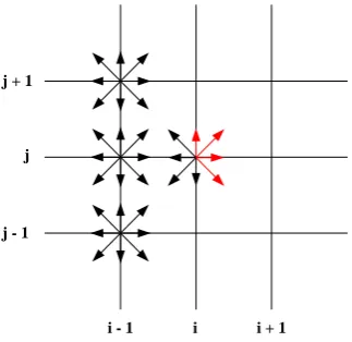
However, the calculation sequence of collision, propagation and macroscopic variables is ambiguous in code implementation. The “pull” and “push” scheme [1] can be used in propagation step. According to the definition, three steps should be computed orderly on all nodes, which means three loops are needed in the programming, and both “pull” and “push” scheme are available. Especially the “pull” scheme, which integrates the three steps into one loop, will be discussed in this paper. The “pull” scheme with one loop is called semi-implicit scheme. In Section 2, Figure 1 will show why we call it “semi-implicit”. The accuracy and efficiency of semi-implicit scheme is discussed in detail through the simulation of lid-driven cavity flow.

Lid-driven cavity flow is a well-known fluid flow problem where the fluid is set into motion by a part of con-taining boundary. This type of flow has been used as a benchmark problem for many numerical methods due to its simple geometry and complicated flow behavior. Ghia et al.[8] give a comprehensive review on the numeri-cal studies related to this type of fluid flows. Hou et al.[9] use LBM for simulating the cavity flow and present solution up to Reynolds number Re = 7500. The results in this paper will be compared with the results of these two articles.

In this paper, Section 2 presents the lattice Boltzmann model used in this study. The standard scheme and semi-implicit scheme of LBM are introduced, and the difference between two schemes is given. Section 3 draws the cavity flow problem, which is simulated by lattice Boltzmann method with semi-implicit scheme. The simu-lation result is compared with the results from previous articles. In addition, the performance comparison be-tween the two schemes is given. Moreover, the final section shows the concluding remarks.

2. Numerical Schemes

2.1. Lattice Boltzmann Method

A lattice Bhatnagar-Gross-Krook (BGK) model [10] [11] is briefly introduced here for the purpose of describing the semi-implicit scheme in the following section. The BGK model is defined by the following equation:

(

)

( )

1 ( )

_{( )}

_{( )}

, , eq , , , 0,1, , 1

j j j j j

f t t t f t f t f t j b

τ 

+ ∆ + ∆ − = _ − _ = _ −

x e x x x (1)

where f_j

( )

x,t is a particle distribution function representing the probability of finding a fluid particle with a velocity e_j at location x and time t. τ is the relaxation time. b is the number of velocities. fj( )eq

( )

x,t is an equilibrium distribution function.

Velocity e_j is determined by a lattice structure. For 2D regular cell models, the most commonly used lattice structure is D2Q9 according to the DdQb notation of Qin et al.[11]. Here, d is the space dimensions, while b

is the number of velocities including the zero velocity, e₀.

j

j - 1 j + 1

i

[image:2.595.235.397.537.694.2]

i - 1 i + 1

The equilibrium distribution function for the D2Q9 lattice model is given by

( )

_{( )}

( )

2 2 2 4 2

9 3

, 1 3

2 2

j j

eq

j j

s s s

t

c c c

ω ρ + + − 

 

 

e u

e u u

f x = (2)

where ω_j is the weight factor in the j direction. The weight factors for the D2Q9 model are 4/9 for the rest particles

(

j=0

)

, 1/9 for particles streaming to the face connected neighbors

(

j=1, 2, 3, 4

)

and 1/36 for par-ticles streaming to the edge connected neighbors

(

j=5, 6, 7,8

)

and while c_s is the speed of sound, and

1 3

s

c = for D2Q9 model. The relaxation time τ is related to the viscosity by

2 1 6

v= τ− (3)

2.2. Boundary Conditions

The boundary condition most commonly used in lattice Boltzmann method is the bounce-back method. The bounce-back scheme is easy to implement and make the method ideal for simulating fluid flows in complicated geometries [8]. However, the bounce-back scheme is only first-order in numerical accuracy at the boundaries, which is not consistent with the order of the LBM in interior points. The non-equilibrium extrapolation scheme is adopted here. The basic idea is to decompose the distribution function into equilibrium part and non-equili- brium part. The scheme is of second-order accuracy in both time and space region [12].

2.3. Difference between Standard and Semi-Implicit Schemes

The macroscopic variables such as density and velocity, which are required for equilibrium distribution function, can be obtained from the following equations:

( )

1 0 , b j j f t ρ − =

=

∑

x (4)

( )

1 0 1 , b j j j f t ρ − = =

∑

u x e (5)

From Equation (1), the fluid particle evolution involves two distinct steps: Collision:

( )

( )

1 ( )

_{( )}

_{( )}

, , eq , , , 0,1, , 1

j j j j

f t f t f t f t j b

τ  

= + _ − _ = −

 x x x x _ (6)

Propagation:

(

,

)

( )

,

j j j

f x+ ∆ + ∆ =e t t t f xt (7)

Macroscopic variables, collision and propagation are the three time consuming steps during the lattice Boltzmann simulation process. The main difference between the standard scheme and semi-implicit scheme in code implementation is that, the former scheme needs three loops for three steps, while the latter scheme needs only one loop in all the nodes for all three steps. When the distribution functions f_j

(

x,t+ ∆t

)

for node

( )

i j, were computed, the distribution functions fjeq

(

x e− ∆j t t,

)

of its neighboring node are used by standard scheme for all directions, but the distribution functions fjeq

(

x− ∆ + ∆ej t t, t

)

of its neighboring nodes are used by semi-implicit scheme for the red directions (shown in Figure 1). The accuracy and efficiency of semi-impli- cit scheme will be discussed through the simulation of cavity flow in the next section.

3. Cavity Simulation and Discussion

257 257× lattice. Initially the velocities at all nodes, except the top nodes, are set to zero. The x-velocity of the top, u is set to 0.1 and the y-velocity is zero. Uniform fluid density ρ =2.7 is imposed initially. The con-vergence criterion for the steady state is given by the follow:

(

) (

2

)

2

1

2 2 1

Er

N

t t t t t t N

t t t t

u u v v

u v

+∆ +∆

+∆ +∆

 _{− + −} 

 _{ <}

 + 

 

∑

∑

(8)

where N is the total number of nodes in the computational domain. u and v are the x-velocity and y-ve- locity respectively.

3.1. Stream Function

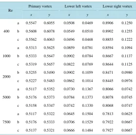
The simulation results computed by semi-implicit scheme were compared with previous works done by Ghia et al.[8] and Hou et al.[9]. First, the locations of primary and secondary vortices are listed in Table 1 and Table 2. The convergence criterion, Er is choosen 10−6 for all simulations.

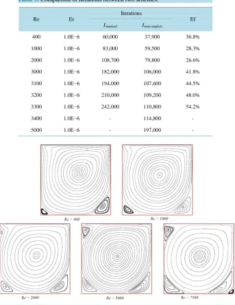
Numerical simulations were carried out for Re=400, 1000, 2000, 5000, 7500. Figure 2 shows the changes of stream function for each Reynolds numbers, the locations of vortices with different level can be seen clearly from these figures, for example, the third level vortices is turned out on the upper left corner of the square cavity when Re=2000. Table 1 shows the locations of the center of primary vortices and the pair of lower vortices for different Reynolds numbers. The locations of the secondary vortex in the upper left corner for Re=5000 and 7500 are listed in Table 2. These result show good agreement with Ghia et al.[8] and Hou et al. [9].

3.2. Performance Compare

For all simulations, steady state is reached when the convergence criterion, Er is less than 10−6 for successive 1000 simulation steps. Table 3 shows the iterations that both schemes are needed. Ef in Table 3 equals

[image:4.595.174.454.432.710.2]

(

Istandard–Isemi-implicit

)

Istandard×100%, which shows the saving proportion of iterative steps of the semi-implicit

Table 1.The locations ,

( )

x y of primary and secondary vortices.

Re

Primary vortex Lower left vortex Lower right vortex

x y x y x y

400

a 0.5547 0.6055 0.0508 0.0469 0.8906 0.1250

b 0.5608 0.6078 0.0549 0.0510 0.8902 0.1255

c 0.5562 0.6063 0.0496 0.0468 0.8855 0.1222

1000

a 0.5313 0.5625 0.0859 0.0781 0.8594 0.1094

b 0.5333 0.5647 0.0902 0.0784 0.8667 0.1137

c 0.5319 0.5657 0.0822 0.0769 0.8644 0.1125

2000

b 0.5255 0.5490 0.0902 0.1059 0.8471 0.0980

c 0.5227 0.5483 0.0862 0.1014 0.8445 0.0976

5000

a 0.5117 0.5352 0.0730 0.1367 0.8066 0.0742

b 0.5176 0.5373 0.0784 0.1373 0.8078 0.0745

c 0.5158 0.5347 0.0742 0.1330 0.8068 0.0747

7500

a 0.5117 0.5322 0.0645 0.1504 0.7813 0.0625

b 0.5176 0.5333 0.0706 0.1529 0.7922 0.0667

c 0.5137 0.5321 0.0666 0.1484 0.7927 0.0667

[image:5.595.144.488.262.707.2]

Table 2.The locations ,

( )

x y of upper left vortex.

Re Upper left vortex

x y

5000

a 0.0625 0.9102

b 0.0667 0.9059

c 0.0634 0.9085

7500

a 0.0664 0.9141

b 0.0706 0.9098

c 0.0669 0.9119

[image:5.595.149.488.264.705.2]

Note: a, Ghia [8] b, Hou [9], c, semi-implicit scheme.

Table 3.Comparison of iterations between two schemes.

Re Er

Iterations

Ef Istandard Isemi-implicit

400 1.0E−6 60,000 37,900 36.8%

1000 1.0E−6 83,000 59,500 28.3%

2000 1.0E−6 108,700 79,800 26.6%

3000 1.0E−6 182,000 106,000 41.8%

3100 1.0E−6 194,000 107,600 44.5%

3200 1.0E−6 210,000 109,200 48.0%

3300 1.0E−6 242,000 110,800 54.2%

3400 1.0E−6 - 114,800 -

5000 1.0E−6 - 197,000 -

[image:6.595.176.458.86.294.2]

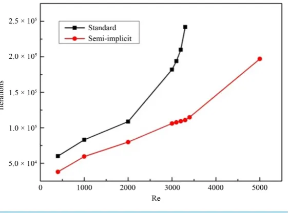
Figure 3.Comparison of iterations between two schemes.

scheme. The iterations can be saved about 30%, when Re less than 3000, and the advantage of semi-implicit scheme becomes more obvious as the Re increases. The standard scheme is not converged once Re > 3400. On the contrary, the iterations of semi-implicit scheme is approximately linear to Re (Figure 3).

4. Conclusion

The essence of semi-implicit scheme is that it uses the latest equilibrium distribution function, computed by the new macroscopic variables. The semi-implicit scheme accelerates the computation rate of flowing status to steady statement and increases the computation efficiency. In addition, the application of semi-implicit scheme is not limited to the cavity flow simulation; many other problems can choose this scheme to reduce the total computing time.

Acknowledgements

We would like to express appreciation to the following financial support: the National Natural Science Founda-tion of China (No. 51490654, 51234007), the NaFounda-tional Natural Science FoundaFounda-tion of Shandong Province (No. ZR2013DL011, No. ZR2014EEP018), China Postdoctoral Science Foundation (No. 2014M551989).

References

[1] Wellein, G., Zeiser, T., Hager, G. and Donath, S. (2006) On the Single Processor Performance of Simple Lattice Boltzmann Kernels. Computers & Fluids, 35, 910-919. http://dx.doi.org/10.1016/j.compfluid.2005.02.008

[2] Ma, J., Wu, K., Jiang, Z. and Couples, G.D. (2010) SHIFT: An Implementation for Lattice Boltzmann Simulation in Low-Porosity Porous Media. Physical Review E, 81, Article ID: 056702.

http://dx.doi.org/10.1103/PhysRevE.81.056702

[3] Skordos, P.A. (1995) Parallel Simulation of Subsonic Fluid Dynamics on a Cluster of Workstations. Proceedings of the Fourth IEEE International Symposium, Washington DC, 2-4 August 1995, 6-16.

[4] Amati, G., Succi, S. and Piva, R. (1997) Massively Parallel Lattice-Boltzmann Simulation of Turbulent Channel Flow.

International Journal of Modern Physics C, 8, 869-877. http://dx.doi.org/10.1142/S0129183197000746

[5] Martys, N.S., Hagedorn, J.G., Goujon, D. and Devaney, J.E. (1999) Large-Scale Simulations of Single- and Multi-component Flow in Porous Media. Proceedings of the International Symposiumon Optical Science, Engineering, and Instrumentation,Denver,18 July 1999, 205-213.http://dx.doi.org/10.1117/12.363723

[6] Tölke, J. (2010) Implementation of a Lattice Boltzmann Kernel Using the Compute Unified Device Architecture De-veloped by nVIDIA. Computing and Visualization in Science, 13, 29-39. http://dx.doi.org/10.1007/s00791-008-0120-2

http://dx.doi.org/10.1016/j.camwa.2009.08.052

[8] Ghia, U.K.N.G., Ghia, K.N. and Shin, C.T. (1982) High-Re Solutions for Incompressible Flow Using the Navier- Stokes Equations and a Multigrid Method. Journal of Computational Physics, 48, 387-411.

http://dx.doi.org/10.1016/0021-9991(82)90058-4

[9] Hou, S., Zou, Q., Chen, S., Doolen, G. and Cogley, A.C. (1995) Simulation of Cavity Flow by the Lattice Boltzmann Method. Journal of Computational Physics, 118, 329-347. http://dx.doi.org/10.1006/jcph.1995.1103

[10] Bhatnagar, P.L., Gross, E.P. and Krook, M. (1954) A Model for Collision Processes in Gases. I. Small Amplitude Processes in Charged and Neutral One-Component Systems. Physical Review, 94, 511-525.

http://dx.doi.org/10.1103/PhysRev.94.511

[11] Qian, Y.H., D’Humières, D. and Lallemand, P. (1992) Lattice BGK Models for Navier-Stokes Equation. Europhysics Letters, 17, 479. http://dx.doi.org/10.1209/0295-5075/17/6/001

[12] Guo, Z.L., Zheng, C.G. and Shi, B.C. (2002) Non-Equilibrium Extrapolation Method for Velocity and Pressure Boun-dary Conditions in the Lattice Boltzmann Method. Chinese Physics, 11, 366-374.