Heuristics For N Job M Machine Flowshop Batch Processing With Breakdown Times

(1)

International Journal of Emerging Technology and Advanced Engineering

Website: www.ijetae.com (ISSN 2250-2459, ISO 9001:2008 Certified Journal, Volume 4, Issue 6, June 2014)

276

Heuristics For N Job M Machine Flowshop Batch Processing

With Breakdown Times

P V Senthiil

1

,

V S Mirudhuneka

2

1

Professor &Head Department of Mechanical Engineering, Saint Peters University, Avadi, Chennai-600054

2_{SAP Technical Consultant, IBM India, DLF tower 1, Chennai-600089, INDIA}

Abstract-- Flow shop scheduling is a typical combinatorial optimization problem, where each job has to go through the processing in each and every machine on the shop floor. Here considered the basic form of flow shop scheduling i.e. Two machine Flow Shop batch processing with type two transportation i.e transportation of jobs from machine shop to dispatch unit. For this problem we investigate the optimal property and propose an algorithm which includes Johnson’s algorithm. After the sequences of jobs are formed we implement breakdown time at two intervals and form another solution. This problem is extended to N job M machine problem to find optimal solution. The performance measure taken here is makes pan and mean weighted flow time of jobs. This type of problem comes under NP hard category.

Keywords-- Flow shop scheduling, Breakdown times, NP hard.

I. INTRODUCTION

Production scheduling is generally considered to be

the one of the most significant issue in the planning

and operation of a manufacturing system. Proficient

scheduling leads to increase in capacity utilization

efficiency and hence thereby reducing the time

required to complete jobs. The main focus of this

paper is scheduling of

N

jobs

M

machine flow shop

batch processing problem with breakdown of

machines. Every batch considered here has common

due date. Initially an efficient algorithm was proposed

for two machine case and the same algorithm was

extended to

M

machine case. After the sequences of

jobs are formed we implement break down times of

machines which is often called preemption according

to algorithm predicted by A.B.Chandramouli.

II. PROBLEM STATEMENT AND NOTATIONS

We consider N job M machine flow shop scheduling batch processing problems with type2 transportations. For this we initially consider two machine n job flow shop scheduling problems and a heuristic solution is formed and the same heuristics is extended to m machine N job scheduling problems.

The flow shop environment consists of N independent jobs N={J1,J2,J3…..Jn} to be processed on two machines M1

and M2.Every job comprises two operations associated with

respective processing times on both machines. Second operation on M2 cannot be started until the first operation is

completed. All the jobs are continuously available at time zero. Every job to be processed is associated with job size Sj and also contains identical due date. In this case

breakdown of machines are occurred in two intervals. After processing in the manufacturing cell, finished jobs are delivered to dispatch section by vehicles. Assume there is only one vehicle available with a limited capacity i.e.) limited batch size. The capacity of vehicle (c) is measured by total physical space that vehicle provides for one delivery. If the sizes of all jobs are equal, the vehicle capacity can be represented by number of jobs. The transporting time from machine shop to dispatch section is denoted by T, which is the sum of t1 and t2, where t1 is the

time taken to travel form machine shop to dispatch section and t2 is the time taken to travel from dispatch section to

machine shop. In most of the cases t1 and t2 are equal. Both

t1 and t2 are independent of the jobs processed. The

breakdown of machines affects only the make span and T is independent from breakdown times.

 P1j – Processing time of jth job in Machine M1

 P2j- Processing time of jth job in Machine M2

 Bk –Batch

 Sj – Jobsize.

 C-Capacity of vehicle.

 Pk-Period of time for processing all jobs in Bk.

 P1k-Sum of processing times on M1 for jobs in Bk.

 P2k- Sum of processing times on M2 for jobs in Bk.

 k – Sum of idle times on M1.

 k -Sum of idle times on M2.

III. LITERATURE SURVEY

(2)

International Journal of Emerging Technology and Advanced Engineering

277

More recently the amount of research devoted to minimization of sum of job completion times has increased. Flow time minimization leads to stable or even use of resources, a rapid turn around of jobs and minimization of in process inventory[6]. Simchi-Levi et al [5] proposes a new worst case results for the bin packing problem. The paper work provides information about the worst case testing for bin packing problems. C.Y.Lee et al [4] investigated machine scheduling models that impose constraints on both transportation capacity and transportation times. From the journals of Lee et al [4], Chang et al [8] the complexity status for two machine flow shop is given as F2(D),k=1|v=1,c|∑Cj is strongly NP hard.

C.Rajendran [3] proposes an efficient heuristic for scheduling in a flow shop to minimize total weighted flow time of jobs. This paper work provides a heuristic approach to find the sequence for optimization of total weighted flow time of jobs.

T.C.E.Cheng et al [7] explains the parallel machine batching problems. He considers a scheduling problem in which n independent and simultaneously available jobs are to be processed on m identical parallel machines. A.B.Chandramouli [6] at 2005 considers a flow shop scheduling problems. It provides a new simple heuristic algorithm for a ‘3-Machine, n job’ flow-shop scheduling problem in which jobs are attached with weights to indicate their relative importance and the transportation time and break down intervals of machine are given. A heuristic approach method to find optimal or near optimal sequence minimizing the total weighted mean production flow time for the problem has been discussed. Guzin ozdagoglu [9] includes a sample case of a sequencing problem of flow shop system for which a simulated annealing algorithm is presented. In addition, the results obtained from the simulated annealing algorithm are compared with the results of scheduling software LEKIN for the same problem. Finally, a simulated annealing algorithm is obtained which is very close to the results of LEKIN which is broadly used within the scheduling applications according to the objective under consideration.

IV. PROOF OF NPHARD

Lemma: 1 The scheduling problem

1(D),k=1|v=1,c=1|∑Cj is NP hard in strong sense.

3-Partition problem

Given a set A={a1,a2,a3,a4….a3m of 3m elements with

positive integer si e s(a) for each a C such that for integer , ( /4) <s(a)< ( /2) and ∑s(a)=m decide if can be partitioned in to m disjoint 3 element subsets A1,A2,A3….. m such that ∑s(a)= for each j=1,2,3,….m.

Lemma: 2 The scheduling problem F2(D)

k=1|v=1,c= |∑Cj is NP hard in strong sense

Proof. With the complexity hierarchy, by setting all of the processing times on M1 orM2 are 0,the scheduling

problem 1(D) k=1|v=1,c= |∑Cj is a special case of the

more general problem F2(D) k=1|v=1,c= |∑Cj. Since 1(D)

k=1|v=1,c= |∑Cj is NP hard in the strong sense, which is

proved in Theorem2, the scheduling problem F2(D) k=1|v=1,c= |∑Cj is also NP-hard in strong sense.

Lemma:3 The scheduling problem F2 (D)

k=1|v=1,c=z|Cmax is NP hard in strong sense.

Consider a special case of F2 (D) k=1|v=1,c=z| Cmax in

which for every job, the processing times of both operations are zero. Hence all of the jobs are ready for delivering to the customer at beginning. In such a case, because of the constant transportation time, minimization of the no. of delivery batches will achieve the optimality and thus the problem can be regarded as a bin packing problem, which is a well-known strongly NP hard problem. Therefore, the problem that we considered is also NP hard in the strong sense.

V. HEURISTICS FOR 2MACHINE FLOW SHOP BATCH

PROCESSING PROBLEMS WITH BREAKDOWN TIMES

Step:1 Assign jobs into batches by First Fit Decreasing algorithm. Set the total number of resulting batches be b,b ≤ n.

Step:2 The jobs within the batches are sequenced using Johnson’s algorithm i.e., SPT(I)-LPT(II) schedule.

Step:3 Calculate the following three values for each batch say Bk in which jobs are scheduled in SPT(I)-LPT(II)

order.

• Δ1 = Φk = Pk – Σ P1j

• Δ2 = ρk = Pk – Σ P2j

• Δ3 = max (Pk-T,0)

Step: 3a Let Sb={B1,B2…. be the set of batches in which

the processing sequence is undecided and another two ordered set S1 and S2 which are both initially empty, be the

set of scheduled batches. Pick the batch from SB with

smallest value over all values obtained in step1.If the value belongs to Δ1, and then set the batch into S1 as the first

element. On the other hand, if the value belongs to Δ2 or

Δ3, then set the batch in to S2 as the last one. Eliminate the

chosen batch from SB.

Step: 3b Iterate step2 until all the batches have its position, i.e., SB is an empty set. Therefore, the permutation of S2 U

(3)

International Journal of Emerging Technology and Advanced Engineering

278

Step: 4 Starting with B1, assign jobs in Bk to the machines,

for K=1,2,….b

Step: 5 Dispatch each completed but undelivered batch whenever the vehicle becomes available. If multiple batches have been completed when the vehicle becomes available, dispatch the batch with the smallest index.

Step:5A : The sequence of batches provides the sequence of overall jobs. Consider the sequence of all jobs and Cmax

value.

Step: 6: Denote the sequence of all jobs as flow time in respective machines. Check for the structural conditions [9].

Step: 7: Implement the effect of breakdown times in the flow time pattern.

Step: 8: Let us consider (a,b) as the breakdown time interval (since deterministic scheduling) then implement the value a to b in the flow processing of the machines.

Step:9: Following Step7 leads to addition of breakdown times on processing time that the job processing in particular machine. This means that the jobs are processed up to the start of the breakdown times and resume the operation after the end of breakdown time.

Step: 10: Update the changes in the changes in the upcoming processing times because the breakdown interval influences the remaining process if the machines.

Step:11 Calculate the mean flow time by using the following formula

Where fi be the flow time of the i th

job, Wi be the

weightage of the ith job

VI. EXTENSION OF ALGORITHM TO NJOBS MMACHINE

FLOW SHOP BATCH PROCESSING WITH BREAKDOWN

TIMES.

Step:1 Assign jobs into batches by First Fit Decreasing algorithm. Set the total number of resulting batches be b,b ≤ n.

Step:2 The jobs within the batches are sequenced using Software based Local search Heuristics algorithm.

Step:3 Calculate the following values for each batch say Bk

in which jobs are scheduled by using Local search Heuristics.

• Δ1 = Pk – Σ P1j

• Δ2 = Pk – Σ P2j

• Δm = Pk – Σ Pmj

• Δm+1 = max (Pk-T,0)

• Where m denotes the no. of machines.

Step: 3 Form Δ’1 and Δ’2 by adding the values of Δ1(m/2)

and Δ2(m/2) .

Step: 4 Let SB={B1,B2…. be the set of batches in which

the processing sequence is undecided and another two ordered set S1 and S2 which are both initially empty, be the

set of scheduled batches. Pick the batch from SB with

smallest value over all values obtained in step1.If the value belongs to Δ’1, and then set the batch into S1 as the first

element. On the other hand, if the value belongs to Δ’2 or

Δm+1, then set the batch in to S2 as the last one. Eliminate

the chosen batch from SB.

Step:5 Iterate step2 until all the batches have its position, i.e., SB is an empty set. Therefore, the permutation of S2 U

S1 is indeed the processing sequence of the batches.

Step: 6 Starting with B1, assign jobs in Bk to the machines,

for K=1,2,….b

Step: 7 Dispatch each completed but undelivered batch whenever the vehicle becomes available. If multiple batches have been completed when the vehicle becomes available, dispatch the batch with the smallest index.

Step: 8: Implement the effect of breakdown times in the flow time pattern.

Step: 8A: Let us consider (a,b) as the breakdown time interval (since deterministic scheduling) then implement the value a to b in the flow processing of the machines.

Step:9: Following Step7 leads to addition of breakdown times on processing time that the job processing in particular machine. This means that the jobs are processed up to the start of the breakdown times and resume the operation after the end of breakdown time.

Step:9A: Update the changes in the changes in the upcoming processing times because the breakdown interval influences the remaining process if the machines.

Step:10: Calculate the mean flow time by using the following formula

(4)

International Journal of Emerging Technology and Advanced Engineering

279

Where fi be the flow time of the ith job

Wi be the weightage of the ith job. Since we are dealing

with mono weightage jobs sum of Wi corresponds to the

total number of jobs.

VII. ILLUSTRATION OF HEURISTIC PROCEDURE

In the previous chapters we proposed the algorithms for

m machine flow shop batch processing with breakdown times. To illustrate the algorithm we select an environment of 10 machine and 20 jobs with common due date and distinct job size. The problem considered here is deterministic nature and all the values are known. The typical data input for the problem is shown here.

 No. of the machine: 10.

 Machine availability: at zero

 Breakdown time: (15-17), (145-147)

 No. of the jobs: 20.

 Job type: Independent jobs.

 Job availability: all are available at zero.

 Environment: Flow shop.

 Sequence: Sequenced as M1 – M2 – M3– M4– M5–

M6– M7– M8– M9– M10

 Earliness cost: 1/unit

 Tardiness cost: 1/unit.

 Weightage of the jobs: Mono weightage jobs.

 Processing: Batch processing.

 Batch size: 20.

 Transportation time to dispatch center: 15.

 Transportation time between the machines: not considered.

 Complexity of the problem: NP hard [chapter 4]

 Performance ratio of the Algorithm: 4 [chapter 6]

 Sub algorithms used:

1. First fit Decreasing Algorithm 2. Software based Local Search Heuristic.

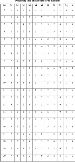
[image:4.612.317.569.147.689.2]

The processing time of each job on machine 1 and machine 2 and the job size of the respective jobs are tabulated as follows.

Table 1

Processing time and job size for m machines

Job

s M

1 M

2 M

3 M

4 M

5 M

6 M

7 M

8 M

9 M1

0 S

j

1 5 2 3 5 7 9 7 8 2 7 3

2 2 6 4 2 6 2 5 2 6 1 4

3 1 2 2 1 3 7 2 5 4 4 2

4 7 5 6 3 2 3 2 4 2 2 1

5 6 6 1 8 6 4 3 9 6 4 4

6 3 7 5 2 2 1 5 3 2 6 3

7 7 2 4 6 5 5 1 2 5 2 2

8 5 1 7 1 7 3 6 6 2 2 1

9 7 8 6 9 1 8 2 1 6 6 4

10 4 3 5 8 3 1 3 8 3 7 5

11 5 2 1 7 6 3 7 5 7 4 2

12 2 6 2 5 6 7 2 1 8 3 3

13 3 4 2 6 1 5 4 7 6 5 4

14 5 2 1 3 8 2 6 1 9 8 3

15 7 6 3 2 6 2 5 7 1 3 2

16 9 2 7 3 4 1 5 3 8 1 1

17 7 5 2 2 3 5 1 6 2 3 3

18 8 2 5 4 9 3 2 6 1 8 4

19 2 6 4 2 6 2 5 2 6 3 5

(5)

International Journal of Emerging Technology and Advanced Engineering

280

The above data are used as input in the algorithm to find Cmax and mean weighted flow time. The major steps in the algorithm are

 Formation of batches – FFD algorithm.

 Sequence of Jobs – Johnson’s algorithm.

 Parameter calculation

 Sequence of batches

 Breakdown implementation

 Flow time calculation.

Step: 1: Formation of batches – FFD algorithm:

Arrange the jobs in non-increasing order of sizes.

• J10-J19- J 2- J 5- J 9- J 13- J 18- J 1- J 6- J 12- J 14- J 17-

J 03- J 07- J 11- J 15- J 20- J 4- J 8- J 16.

• Formation of batches by First Fit Decreasing algorithm

• B1={J10,J19,J2,J5,J3} Batch

size=20

• B2={J9,J13,J18,J1,J6,J7} Batch

size=20

• B3={J12,J14,J17,J11,J15,J20,J4,J8,J10} Batch size=18

In the jobs from 1 to 20 J10 and J19 are the jobs having

highest job sizes hence are placed in the top places of the batch 1.The total batch size of the processing is 58.Hence 20 jobs forms three batches exactly. The last batch B3 is the

only batch which has the batch size as 18.But during the transportation B3 is also considered equivalent to other

batches. The batches B1, consists of only 5 jobs while the

batches B2 consists of 6 jobs and B3 consists of 9 jobs . In

this the batch B3 consists the jobs with very low job size in

the processing cell.

Step:2: Sequence of jobs within the batches.

Hence the problem is Fm||Cmax and from many

researches it is proved that Local search Heuristic provides the optimal solution to these kind of problems. So we use Local search Heuristic rule for the sequence of jobs within each batch.Sequence of Batch B1: B1={J10,J19,J2,J5,J3},

Batch size=20

Fig1 Gantt chart for sequence of jobs within the batch 1

By applying Local search Heuristic we obtain Cmax = 65

Job sequence = J03 – J19 – J05– J10– J02.

• Sequence of Batch B2: B2={J9,J13,J18,J1,J6,J7}

[image:5.612.334.560.143.310.2]

Batch size=20

Fig 2 Gantt chart for sequence of jobs within the batch 2

By applying Local search Heuristic we obtain Cmax =

78.

Job sequence = J13 – J01 – J06– J18– J09– J07.

Sequence of Batch B2:

B3= {J12, J14, J17, J11, J15, J20, J4, J8, J10}

Batchsize=18

Fig 3 Gantt chart for sequence of jobs within the batch 3

By applying Local search Heuristic we obtain Cmax =

83.

Job sequence = J14 – J08 – J11– J12– J17– J15– J20– J16– J04.

Step:3: Parameter Calculation:

Calculate the following values for each batch say Bk in

which jobs are scheduled by using Local search Heuristics.. • Δ1 = Pk – Σ P1j

• Δ2 = Pk – Σ P2j

• Δm = Pk – Σ Pmj

• Δm+1 = max (Pk-T,0)

• Where m denotes the no. of machines.

• Form Δ’1 and Δ’2 by adding the values of Δ1(m/2)

and Δ2(m/2) .

• Where, Pk-Period of time for processing all jobs in

[image:5.612.52.286.607.716.2]

(6)

International Journal of Emerging Technology and Advanced Engineering

281

• P1k-Sum of processing times on M1 for jobs in Bk.

• P2k- Sum of processing times on M2 for jobs in Bk.

• Δ1 – Sum of idle times on M1.

• Δ2 –Sum of idle times on M2.

• Δm –Sum of idle times on Mm.

• T- Transportation time

From these values only we can sequence the set of batches formed through FFD algorithm. Here the transportation time is 15.Hence for the m machine flow shop scheduling batch processing problem the values are tabulated as follows.

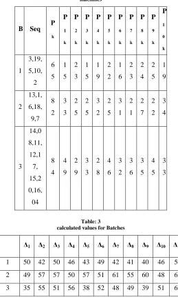
Table 2

List of sequence of batch and processing time of jobs in respective machines

B Seq P

k

P

1

k

P

2

k

P

3

k

P

4

k

P

5

k

P

6

k

P

7

k

P

8

k

P

9

k

P

1

0

k

1 3,19,

5,10,

2 6

5 1

5 2

3 1

5 1

9 2

2 1

6 2

3 2

4 2

5 1

9

2 13,1,

6,18,

9,7 8

2 3

3 2

5 2

5 3

2 2

5 3

1 2

7 2

2 3

4

3 14,0

8,11,

12,1

7,

15,2

0,16,

04 8

4 4

9 2

9 3

3 2

8 4

6 3

2 3

6 3

5 4

5 3

[image:6.612.363.523.171.277.2]

3

Table: 3 calculated values for Batches

Δ1 Δ2 Δ3 Δ4 Δ5 Δ6 Δ7 Δ8 Δ9 Δ10 Δ11

1 50 42 50 46 43 49 42 41 40 46 50

2 49 57 57 50 57 51 61 55 60 48 67

3 35 55 51 56 38 52 48 49 39 51 69

Let us form Δ’1 and Δ’2 by adding the values of Δ1(m/2)

[image:6.612.50.290.292.729.2]

and Δ2(m/2)

Table 4

Summation of Δ1(m/2) and Δ2(m/2)

Δ’1 Δ’2 Δ11

231 218 50

270 275 67

235 239 69

Step:4: Sequence of batches

Establish SB = {B1, B2, B3}.S2 U S1 = {} which is an

empty set. From the table, the smallest value is 50 which lies in both ∆11. Hence place B1 at the end of S2 i.e.) S2 =

{B1}. Remove that batch from SB. Then the repeat the

procedure until SB becomes an empty set. Hence the

optimal batch sequence is S2 U S1 i.e.) B3-B2-B1.It means

that the overall sequence of the jobs to be processed in the machines is J14 – J08 – J11-J12 – J17 – J15– J20 –J16 – J04 – J17

-J13– J01 – J06-J18 –J09– J07 – J03-J19 -J05 – J10 – J02..By

following this a Gantt chart is obtained. The value of Cmax

[image:6.612.36.295.295.726.2]

obtained through the proposed algorithm is 164.

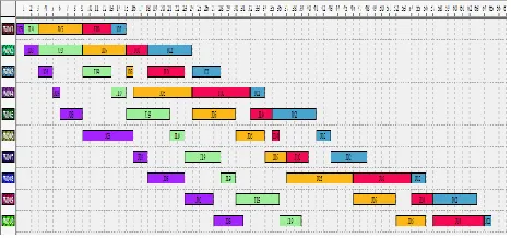
Fig 4 Overall sequence of jobs in three batches.

Hence Cmax = 164.

Completion time for B3= 86.

Common Due date of the batches = 135 Early Batches = B3.

Tardy Batches =B1, B2.

JIT Batch = B6

Early cost = 49 Tardy cost = 6+29=35. Total cost = 35+49=84. Total completion time = 164.

(7)

International Journal of Emerging Technology and Advanced Engineering

282

Step: 5: Breakdown implementation:

For the implementation of breakdown we have to formulate the optimal sequence as typical flow pattern. In our problem breakdown times are implemented in two intervals as (15-17) and (145-147) [since deterministic scheduling] .Initial step of break down calculation is sequence of jobs optimally. That we have done at the end of Step:4. as is J14 – J08 – J11-J12 – J17 – J15– J20 –J16 – J04 –

J17 -J13– J01 – J06-J18 –J09– J07 – J03-J19 -J05 – J10 – J02.Second

step is to denote the sequence as flow time in the machines

Table: 5

Flow time of jobs in respective machines

Jo

b M

1

M2 M3 M4 M5 M6

M

7

M

8

M9 M10

1 4 0-5 5-7 7-8 8-11 11-19 19 -21 2 1 -2 7 2 7 -2 8 28 -37 37-45 0 8 5-1 0 10 -11 11 -18 18 -19 19-26 26 -29 2 9 -3 5 3 5 -4 1 41 -43 45-47 1 1 1 0-1 5 15 -17 18 -19 19 -26 26-32 32 -35 3 5 -4 2 4 2 -4 7 47 -54 54-58 1 2 1 5-1 7 17 -23 23 -29 29 -34 34-40 40 -47 4 7 -4 9 4 9 -5 0 54 -62 62-65 1 7 1 7-2 24 -29 -34 - 40-43 47 -5 2 -5 3 -62 -65-68

4 29 31 36 52 5

(8)

International Journal of Emerging Technology and Advanced Engineering

(9)

International Journal of Emerging Technology and Advanced Engineering

284

The jobs which are affected by implementation of breakdown times are highlighted.

J14 on M5,J08 on M3,J11 on M2,J12 on M1,J19 on M10,J05 on

M9,J10 on M8

The initial breakdown causes some changes in second one.

Implementation of Breakdown times:

Table: 6

Flow time of jobs with breakdown in respective machines.

Jo

b M1 M2 M3 M4 M5 M6 M7 M8 M9 M1 0 1 4 0-5 5-7 7-8 8-11 11 -21 21 -23 23 -29 29 -30 30 -39 39 -47 0 8 5-10 10 -11 11 -20 20 -21 21 -28 28 -31 31 -37 37 -43 43 -45 47 -49 1 1 10 -15 15 -19 20 -21 21 -28 28 -34 34 -37 37 -44 44 -49 49 -56 56 -60 1 2 15 -19 19 -25 25 -31 31 -36 36 -42 42 -49 49 -51 51 -52 56 -64 64 -67 1 7 19 -26 26 -31 31 -33 36 -38 42 -45 49 -54 54 -55 55 -61 64 -66 67 -70 1 5 26 -33 33 -39 39 -42 42 -44 45 -51 54 -56 56 -61 61 -68 68 -69 70 -73. 2 0 33 -40 40 -41 42 -46 46 -48 51 -55 56 -62 62 -64 68 -70 70 -76 76 -83

1 40 49 51 58 61 65 66 71 76 84

6

(10)

2-International Journal of Emerging Technology and Advanced Engineering

285

3 90 94 10

2 11

9 12

8 13

0 13

5 13

9

14

8

1

9 90

-92 94

-10

0 10

2-10

6 11

2-11

4 11

9-12

5 12

8-13

0 13

0-13

5 13

5-13

7 13

9-14

5 14

8-15

1

0

5 92

-98 10

0-10

6 10

6-10

7 11

4-12

2 12

5-13

1 13

1-13

5 13

5-13

8

13

8-14

9

14

9-15

5 15

5-15

9

1

0 98

-10

2 10

6-10

9 10

9-11

4 12

2-13

0 13

1-13

4 13

5-13

6 13

8-14

1 14

9-15

7 15

7-16

0 16

0-16

7

0

2 10

2-10

4 10

9-11

5 11

5-11

9 13

0-13

2 13

4-14

0 14

0-14

2

14

2-14

9

15

7-15

9 16

0-16

6 16

7-16

8.

Hence Cmax = 168

Common Due date of the batches = 135 Early Batches = B3.

Tardy Batches =B1, B2.

Early cost = 47

Tardy cost = 7+33= 40.

Total cost = 40+47=87.

Calculation of Total flow time for m machine without breakdown:

∑wi fi=

45+(47-5)+(58-10)+(65-15)+(68-17)+(71-24)+(81-31)+(83-38)+(86-

47)+(102-54)+(119-57)+(125- 62)+(133-65)+(139-73)(141-80)+(145-87)+(148-88)+(155-90)+(163-96)+(164-100).

=45+42+48+50+51+47+50+45+39+48+62+63+68+66+61 +58+60+65+67+64.

=1099.

∑wi fi= 1099

Fw= 1099/20 = 54.95.

Calculation of Total flow time for m machine with breakdown:

∑wi fi=

47+(49-5)+(60-10)+(67-15)+(70-19)+(73- 26)+(83-33)+(85-40)+(88-49)+(104-56)+(120-59)+(126- 64)+(134-67)+(140-75)+(142-82)+(148-89)+(151-90)+(159-92)+(167-98)+(168-102)=

47+44+50+52+51+47+50+45+39+48+61+62+67+65+60+5 9+61+67+69+66

=1110

∑wi fi= 1110.

Fw= 1110/20 = 55.5.

VIII. CONCLUSION

(11)

International Journal of Emerging Technology and Advanced Engineering

286

All the Gantt charts are made with the help of Lekin scheduling systems. Lekin provides the solution for m machine problems through Local search Heuristics method. Another software tool used in our paper is Lisa (Library of Scheduling Systems) to find the optimality. Hence we complete our objective in our paper successfully.

REFERENCE

[1 ] Johnson.S.M. Optimal two and three stage production schedules with setup time included., Naval Research Logistics Quartly1(1954) 61-68.

[2 ] Garey.M.R,Johnson.D.S.,The Complexity of Flow shop and Job shop scheduling, Mathematics of operations research 1 (1976) 117-129.

[3 ] Rajendran.C.,Zeigler.H., An efficient heuristics for scheduling in a flow shop to minimize total weighted flow time of jobs.

[4 ] Lee.C.Y., Chen.Z.L. Machine scheduling with deliveries to multiple customer locations, European Journal of Operational Research 164(2005) 39-51.

[5 ] Simchi- Leve.D ., New worst case results for bin-packing problem, Naval Research Logistics 41 (1994) 579-585.

[6 ] A.B.Chandramouli., Heuristic approach for N job 3 machine flow shop scheduling problem involving transportation time, Breakdown times and Weightage of jobs., Mathematical and Computer application vol 10 pp.301-305,2005.

[7 ] T.C.E. Cheng, Z.-L. Chen, M.Y. Kovalyov and B.M.T. Lin, Parallel-machine batching and scheduling to minimize total completion time, IIE Transactions 28 (1996) 953-956.

[8 ] Chang.Y.C et al Machine scheduling with job deliver coordination, European Journal of Operational Research 158 (2004) 470-487. [9 ] Guzin ozdagoglu A simulated annealing application on flow shop