Optimizing and analysing returns in commodity trading using Genetic Algorithm, Simulated Annealing and a novel algorithm (GaSa)

(1)

International Journal of Emerging Technology and Advanced Engineering

Website: www.ijetae.com (ISSN 2250-2459,ISO 9001:2008 Certified Journal, Volume 2, Issue 12, December 2012)

662

Optimizing and analysing returns in commodity trading using

Genetic Algorithm, Simulated Annealing and a novel algorithm

(GaSa)

G.Anuradha

1,

Dimple Bohra

2

1

Associate Professor, St.Francis Institute of Technology,Borivli(West)Mumbai, Maharashtra, India. 2

M.E. (Computer Engineering) Student of Thadomal Shahani Engineering College, Mumbai, Maharashtra, India.

Abstract— Commodity trading or future trading is the trading on commodities. It is more stable than stock trading although is associated with greater risk factors. This paper proposes a novel algorithm GaSa for optimizing the returns in commodity trading. This novel algorithm hybridizes Genetic Algorithm and Simulated Annealing, with the mutation phase of Genetic algorithm replaced by simulated annealing. Results have shown that in comparison to using Genetic Algorithm, Simulated Annealing, GaSa produces optimized values with lesser number of iterations and also taking lesser time. The inputs to the system are the opening price, closing price and the Volume of commodities traded from Multi-Commodity Exchange (MCX), India..

Keywords—Genetic Algorithm(GA), Simulated Annealing (SA), GaSa(Hybridized Genetic Algorithm and Simulated Annealing)

I. INTRODUCTION

A commodity is a product having commercial value that can be produced, bought, sold, and consumed. Commodities are consistently produced by large number of manufacturers to fulfil the needs of entire population; Examples of commodities includes items like oil, wheat and corn. Commodity trading is separate from the trading of other securities. There are separate exchanges for commodity trading. There are commodity trading exchanges all over the world. The price of commodities is determined by the laws of supply and demand. If a natural disaster wipes out a large amount of any commodity the supply will come down, resulting in a price hike. An investor in this commodity would make money in this scenario. Likewise, if for whatever reason a commodity becomes less in demand suddenly, investors might lose money. However, as you can imagine, these dire scenarios do not happen all that often since commodities are generally necessities.

This makes commodity trading, in general more stable than trading other types of securities such as stocks.

Commodity future is a contract to buy or sell specific commodity, of a specific quality, at a specific price, for a specific future date on the exchange. A forward contract is a legally enforceable agreement for delivery of goods or the underlying asset on a specific date in future at a price agreed on the date of contract. Commodities future contract is an agreement to buy or sell a set amount of commodity at a predetermined price and date. Buyers use these to avoid the risks associated with the price fluctuations of the product or raw material, while sellers try to lock in a price for their products. Like in all financial markets, others use such contracts to gamble on price movements [1]

For the past decade and half immense work is done in the field of machine learning to maximize profits, predicting returns in financial markets. Genetic algorithms provide an excellent way to maximize a function. They allow for searching broad, poorly understood solution spaces and finding maximizing values for function parameters [2].

For optimizing the returns input data taken from MCDEX is evaluated using Genetic Algorithm, Simulated Annealing and GaSa (novel architecture of Genetic and Simulated Annealing).

II. EVOLUTIONARY OPTIMIZATION ALGORITHMS

During the last few decades, stock traders have largely been relying on various types of intelligent systems to make trading decisions. Evolutionary algorithms like Genetic Algorithm and Simulated Annealing is extensively used for trading and optimizing purposes. The algorithms used for optimizing returns are

Genetic Algorithms (GA) Simulated Annealing (SA)

(2)

International Journal of Emerging Technology and Advanced Engineering

663

2.1 Genetic Annealing (GA)

GA is a family of computational models inspired by evolution. These algorithms encode a potential solution to a specific problem on a simple chromosome-like data structure, and apply recombination operators to these structures in such a way as to preserve critical information. In general, the implementation of a GA begins with a population of random chromosomes. One then evaluates these structures and allocated reproductive opportunities in such a way that those chromosomes which represent a better solution to the target problem are given more chances to ‗reproduce‘ than those chromosomes which are poorer solutions. The ‗goodness‘ of a solution is defined with respect to the current population [3].

The GA in this case works as follows

The population of chromosomes: In this case the proportion of each commodity to be invested is a single chromosome. There are 10 commodities considered for optimization. So the initial population size becomes 50x10.

Fitness function:

(1)

𝑓 𝑥 = 𝑥 𝑖 ∗ 𝑟(𝑖)

𝑛

𝑖=1

Subject to the constraint such that

𝑥 𝑖 = 1

𝑛

𝑖=1

𝑥 𝑖 ≥ 0

Where n=total number of commodities and

x(i)=proportion of ith commodity to be invested and r(i)=expected return of the ith commodity

Selection of chromosomes:

a. Roulette wheel: A common selection approach assigns a probability of selection Pj to each individual j based on its fitness value. A series of N random numbers is generated and compared against the cumulative probability.[4] The cumulative probability is given by

Ci= 𝑖 𝑃𝑗

𝑗 =1 (2)

of the population. The appropriate individual i is selected and copied into the new population if Ci-1 < U (0, 1) ≤ Ci. This process is repeated till the population size is same as the initial population size (50x10).

b. Tournament Selection: The tournament selection selects chromosomes from initial population based on the tournament held between s initial chromosomes, where s is the tournament size which is randomly selected. The winner from this selection will be the one with highest fitness value and will be inserted into the mating pool.

Just like Roulette wheel selection, this process is also repeated till the population size is same as the initial population size (50x10).

4. Crossover: In the crossover operator, new strings are created by exchanging information among strings of the mating pool. Many crossover operators exist in the GA literature like single point crossover, two point crossover, arithmetic crossover etc.

a. A single - point crossover operator is performed by randomly choosing a crossing site along the string and by exchanging all the elements on the right side of the crossing site as shown:

0.08 0.42 0.07 0.01 0.16|0.08 0.15 0.12 0.01 0.06 0.12 0.05 0.08 0.12 0.09|0.15 0.02 0.15 0.12 0.04

O1 0.08 0.42 0.07 0.01 0.16 0.15 0.02 0.15 0.12 0.04 O2 0.12 0.05 0.08 0.12 0.09 0.08 0.15 0.12 0.01 0.06

O1 and O2 are the newly formed chromosomes after single point crossover. Fitness function is applied to O1 and O2. The one with highest fitness value goes to the next operation Mutation.

b. Arithmetic Crossover: Arithmetic crossover is also applied on selected chromosomes from initial population. In arithmetic crossover, two chromosomes xn1 and xn2 are randomly selected; a random number c ∈U (0, 1) is generated. Crossover operation is carried out according to the rules as given by eqn

xm1= c * xn1 + (1-c) * xn2 (3) xm2= c * xn2 + (1-c) * xn1 (4) where xm1 and xm2 are the newly formed chromosomes after arithmetic crossover. Fitness function is applied to xm1 and xm2. The one with highest fitness value goes to the next operation mutation.

5. Mutation: In Mutation randomly two positions in the chromosomes as a resultant of crossover is selected and the positions are swapped.

6. The termination criteria are checked. This is either the maximum number of iterations or the error value which is the difference between the fitness value of the present and the previous iterations. In the present scenario the termination criteria is either 100 iterations or error value is less than or equal to -1. Finally the optimal chromosome with maximum fitness value is displayed. In this case the portfolio which has the optimized returns is selected as the resultant of GA.

2.2 Simulated Annealing (SA)

(3)

International Journal of Emerging Technology and Advanced Engineering

664 SA is a generic name for a class of optimization heuristics that perform a stochastic neighborhood search of the solution space. The major advantage of SA over classical local search methods is its ability to avoid getting trapped in local minima while searching for a global minimum. And it is a single point search method.

The basic principle of the SA heuristic can be described as follows.

Step 1: Initialization

Initialize the iteration count k = 0, and the temperature T0 to be sufficiently high. Find an initial solution.

Step 2: Repeat for each temperature Tk

Execute Steps 3-5 until an equilibrium criterion is satisfied.

Step 3: Neighborhood solution

Generate a trial solution xk+1 in the neighborhood of the current solution xk.

Step 4: Acceptance criterion

Let

Δ= f(xk+1) – f (xk) (5)

And r is a random number uniformly distributed over [0,1]. If Δ< 0 (i.e., the solution is improved), the trial solution is accepted. Otherwise, the trial solution is accepted with the probability

exp (-Δ/Tk) > r

Step 5: Cooling schedule

Gradually decrease the value of the temperate Tk by Tk+1 = p* Tk, 0 < p < 1

Steps 6: Convergence check

It the number of the accepted solution is small enough, freezing point is reached and the algorithm is terminated. Otherwise, set k=k+1 and go to Step 2.

2.3 Novel Algorithm (GaSa)

In GaSa the mutation phase of Genetic algorithm is replaced by Simulated Annealing.

III. IMPLEMENTATION

The data for the proposed algorithm GaSa is taken from MCXIndia.com website. The opening price, closing price, volume of all the commodities irrespective of different portfolios is taken. The number of commodities is restricted to a maximum of ten. This is accomplished by taking one from each of the categories of portfolios. The return computed using [1] is modified as per the commodity market parameter. So in this case the volume traded is used for computing the returns.

Return = (cp-op/op)*V (6)

Where cp=closing_price; op=opening_price; V=Volume

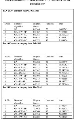
TABLEI

SAMPLE INPUTS FOR JAN 2009 WITH CONTRACT EXPIRY DATE FEB 2009

Date Sym bol

Exp.M

on Open Close Vol Ret N return

01- Jan-09 AL

27-Feb-09

74.4

5 74.65 13 0.03 0.999 01- Jan-09 CAR D

14-Feb-09 556 554 2

-0.01 0.999 01- Jan-09 CHA N

20-Feb-09 2040 2074 237 3.95

0.97331 6 01- Jan-09 COR IAN DER

14-Feb-09 4370 4375 2 0

0.99966 6 01- Jan-09 CRU DEO IL

13-Feb-09 2273 2284 3888 18.8 2 0.87411 6 01- Jan-09 GOL DM 05-Feb-09 1360

0 13714 1787

7 149.

85 0

01- Jan-09 KAP ASK HAL I

28-Feb-09 461 460.1 27

-0.05 1

01- Jan-09 LEA D 27-Feb-09 50.5

5 51.1 72 0.78

0.99446 3 01- Jan-09 NAT URA LGA S 20-Feb-09 275.

5 276.5 50 0.18

0.99846 6 01- Jan-09 ZIN C

27-Feb-09 60.4 60.55 101 0.25

0.99799 9 Maximum Return : 149.85

Minimum Return : -0.05

(4)

International Journal of Emerging Technology and Advanced Engineering

665 Where i=1..n n being the number of commodities

By using equation 7 the range of returns can be normalized between 0 and 1. These inputs are used in three different algorithms

The input data is taken from MCDEX site for two year Jan 2009 and Jan 2010. The Inputs are restricted to 10 commodities one belonging to each classification of Petroleum Commodities, Industrial Metal Commodities, Precious Metal Commodities, Livestock Commodities, Agriculture Commodities. Initial population size is 50*10. The return, normalized return is computed using equations 6 and 7 respectively. This becomes the input to each of the 3 algorithms.

In GA the fitness function is computed using both Roulette Wheel and Tournament Selection for Selection phase and Single point Cross over and Arithmetic Crossover for the Crossover phase. The algorithm is executed till the termination criteria are reached.

In SA after computing the normalized return using equation 7 the SA is evaluated with initial temperature to be 1000, K to be equal to 10, lamda equal to 0.5, maximum number of iterations to be 100, error criteria to be -1 and the termination criteria or freezing point to be 5.

In GaSa the same input and the specifications of GA is taken with only the mutation phase of GA being replaced by SA.

IV. RESULTS AND ANALYSIS

The results are done for all the different combinations

Genetic Algorithm with Roulette Wheel selection and single point Crossover (GA+RW+SP)

Genetic Algorithm with Roulette Wheel selection and Arithmetic Crossover (GA+RW+AC)

Genetic Algorithm with Tournament Selection and Single point Crossover (GA+TS+SP)

Genetic Algorithm with Tournament Selection and Arithmetic Crossover (GA + TS +AC)

Simulated Annealing (SA)

GaSa with Roulette Wheel Selection and Single Point Crossover (GaSa+RW+SP)

GaSa with Roulette Wheel selection and Arithmetic Crossover (GA+RW+AC)

GaSa with Tournament Selection and Single point Crossover (GA+TS+SP)

GaSa with Tournament Selection and Arithmetic Crossover (GA + TS +AC)

[image:4.612.314.571.254.670.2]

The results obtained for the period Jan2010 and Feb 2012 are tabulated in table 2

TABLE II. SAMPLEINPUTSFORJAN2009WITHCONTRACTEXPIRY DATEFEB2009

JAN 2010- contract expiry JAN 2010

Sr.No. Name of algorithm

Highest fitness

Iteration time

1 SA 0.9346 23 1.608243

2 GA+RW+SP 0.9487 80 7.738410

3 GA+RW+AC 0.9361 91 11.393233

4 CA+RW+SP 0.9637 36 8.207187

5 CA+RW+AC 0.9372 45 7.508876

Jan2010- contract expiry date Feb2010

Highest fitness

Iteration time

1 SA 0.9382 31 1.285849

2 GA+RW+SP 0.9418 80 13.090827

3 GA+RW+AC 0.9321 89 12.277763

4 GA+TS+SP 0.9542 69 77.345318

5 GA+TS+AC 0.9356 51 75.780455

6 CA+RW+SP 0.9493 36 8.106205

7 CA+RW+AC 0.9373 41 7.806369

8 CA+TS+SP 0.9695 94 78.437777

9 CA+TS+AC 0.9352 64 80.730169

Jan2010- contract expiry date Mar2010

Highest fitness

Iteration time

1 SA 0.9269 20 1.498244

2 GA+RW+SP 0.9409 64 8.406521

3 GA+RW+AC 0.9260 95 11.289517

4 CA+RW+SP 0.9526 32 7.898222

(5)

International Journal of Emerging Technology and Advanced Engineering

[image:5.612.62.273.130.211.2]

666

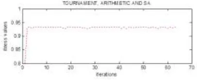
[image:5.612.53.285.262.351.2]

Figure I: Optimizing fitness function using tournament selection and single point crossover

Figure II: Optimizing fitness function using tournament selection and arithmetic crossover

Figure III: Optimizing fitness function using Combined approach GaSa with tournament selection and single point crossover

For the inputs taken in table 1 the results are arrived for different contract expiry dates. The following observations are seen from the above table.

Figure IV: Optimizing fitness function using Combined approach GaSa with tournament selection and arithmetic crossover

The comparisons can be made on different grounds

1. Based on the time taken to execute different algorithms

2. Fitness value

3. Number of iterations.

Although commodity trading expires in different expiry periods, it has no effect on the fitness value computed. The fitness values for different expiry periods and for different combinations of algorithms fetch almost similar values. With respect to the time taken for executing different algorithms, and also the number of iterations taken, Genetic algorithm takes comparatively more number of iterations irrespective of the selection and crossover methods used .

V. CONCLUSION

GaSa results are comparatively better than GA with respect to the number of iterations and the time taken.

GA is a parallel search optimization technique and is arrives at global optimum. SA arrives at a single point optimization technique. Search space of GA is much more than that of SA. So GA produces better optimization than SA. But despite the above advantage, GA gets stuck up in local minima. This problem is avoided using SA in the mutation phase of GA. This is evident from the graphs shown in Figure IV

REFERENCES

[1] http://www.investopedia.com/terms/c/commodityfuturescontract.asp

[2] Ernest A. Foster, ―Commodity Futures Price Prediction, an Artificial Intelligence Approach‖, B.S., The University of Alabama, 1993

[3] Darrell Whitley, ―A genetic algorithm tutorial‖, Computer Science Department, Colorado State University, Fort Collins, CO 80523, USA, Statistics and Computing (1994) 4, 65-85

[image:5.612.60.275.404.496.2] [image:5.612.66.269.572.655.2]