What said the neoclassical and endogenous growth theories about Portugal?

(1)

What said the neoclassical and

endogenous growth theories about

Portugal?

Martinho, Vítor João Pereira Domingues

Escola Superior Agrária, Instituto Politécnico de Viseu

2011

Online at

https://mpra.ub.uni-muenchen.de/32631/

(2)

WHAT SAID THE NEOCLASSICAL AND ENDOGENOUS GROWTH

THEORIES ABOUT PORTUGAL?

Vitor João Pereira Domingues Martinho

Unidade de I&D do Instituto Politécnico de Viseu Av. Cor. José Maria Vale de Andrade

Campus Politécnico 3504 - 510 Viseu

(PORTUGAL)

e-mail: vdmartinho@esav.ipv.pt

ABSTRACT

The aim of this paper is to present a further contribution, with panel data, to the analysis of absolute convergence (



and



), associated with the neoclassical theory, and conditional, associated with endogenous growth theory, of the sectoral productivity at regional level. Presenting some empirical evidence of absolute convergence of productivity for each of the economic sectors in each of the regions of mainland Portugal (NUTS III) in the period from 1995 to 1999. They are also presented empirical evidence of conditional convergence of productivity, for each of the economic sectors of the NUTS II of Portugal, from 1995 to 1999. The structural variables used in the analysis of conditional convergence is the ratio of capital/output, the flow of goods/output and location ratio. This study analyses, also, through cross-section estimation methods, the influence of spatial effects and human capital in the conditional productivity convergence in the economic sectors of NUTs III of mainland Portugal between 1995 and 2002. This study analyses, yet, through cross-section estimation methods, the influence of spatial effects in the conditional product convergence in the parishes’ economies of mainland Portugal between 1991 and 2001. The conclusions depend of the period and of the method used.

Keywords: convergence; spatial econometrics; Portuguese regions

1. EMPIRICAL EVIDENCE OF ABSOLUTE CONVERGENCE, PANEL DATA

The purpose of this part of the work is to analyze the absolute convergence of output per worker (as a "proxy" of labor productivity), with the following equation ((1)Islam, 1995, based on the (2)Solow model, 1956):

it t i it

c

b

P









ln

_,_₁ (1)

Are presented subsequently in Table 1 the results of the absolute convergence of output per worker, obtained in the panel estimations for each of the sectors and all sectors, now at the level of NUTS III during the period 1995 to 1999 ((3)Martinho, 2011a).

[image:2.595.71.530.573.767.2]

The results of convergence are statistically satisfactory for all sectors and for the total economy of the NUTS III.

Table 1: Analysis of convergence in productivity for each of the economic sectors at the level of NUTS III of Portugal, for the period 1995 to 1999

Agriculture

Method Const. Coef. T.C. DW R2 G.L. Pooling 0.017

(0.086)

-0.003

(-0.146) -0.003 2.348 0.000 110

LSDV -0.938*

(-9.041) -2.781 2.279 0.529 83

GLS -0.219* _(-3.633) 0.024* _(3.443) 0.024 1.315 0.097 110 Industry

Method Const. Coef. T.C. DW R2 G.L. Pooling 0.770*

(4.200)

-0.076*

(-4.017) -0.079 1.899 0.128 110

LSDV -0.511*

(-7.784) -0.715 2.555 0.608 83

GLS 0.875* (4.154)

-0.086*

(-3.994) -0.090 2.062 0.127 110

Services

Method Const. Coef. T.C. DW R2 G.L. Pooling 0.258

(1.599)

-0.022

(-1.314) -0.022 1.955 0.016 110

LSDV -0.166*

(3)

GLS 0.089 (0.632)

-0.004

(-0.303) -0.004 1.868 0.001 110

All sectors

Method Const. Coef. T.C. DW R2 G.L.

“Pooling” 0.094 _(0.833) -0.005 _(-0.445) -0.005 2.234 0.002 110

LSDV -0.156*

(-3.419) -0.170 2.664 0.311 83

GLS 0.079 (0.750)

-0.004

(-0.337) -0.004 2.169 0.001 110

Note: Const. Constant; Coef., Coefficient, TC, annual rate of convergence; * Coefficient statistically significant at 5%, ** Coefficient statistically significant at 10%, GL, Degrees of freedom; LSDV, method of fixed effects with variables dummies; D1 ... D5, five variables dummies corresponding to five different regions, GLS, random effects method.

2. EMPIRICAL EVIDENCE OF CONDITIONAL CONVERGENCE WITH PANEL DATA

This part of the work aims to analyze the conditional convergence of labor productivity sectors (using as a "proxy" output per worker) between the different NUTS II of Portugal, from 1995 to 1999.

[image:3.595.60.542.338.688.2]

Given these limitations and the availability of data, it was estimated in this part of the work the equation (1) introducing some structural variables, namely, the ratio of gross fixed capital/output (such as "proxy" for the accumulation of capital/output ), the flow ratio of goods/output (as a "proxy" for transport costs) and the location quotient (calculated as the ratio between the number of regional employees in a given sector and the number of national employees in this sector on the ratio between the number regional employment and the number of national employees) ((4) Sala-i-Martin, 1996).

Table 2: Analysis of conditional convergence in productivity for each of the sectors at NUTS II of Portugal, for the period 1995 to 1999

Agriculture

Method Const. D1 D2 D3 D4 D5 Coef.1 Coef.2 Coef.3 Coef.4 DW R2 G.L.

Pooling 0.114 (0.247) -0.020 (-0.392) 0.388 (0.592) 0.062 (1.267) -0.062

(-1.160) 2.527 0.136 15

LSDV 5.711*

(2.333) 5.856* (2.385) 6.275* (2.299) 6.580* (2.383) 6.517* (2.431) -0.649* (-2.248) -0.134 (-0.134) -0.132 (-0.437) -0.102

(-0.189) 2.202 0.469 11 GLS -0.020

(-0.221) -0.004 (-0.416) 0.284 (1.419) 0.059* (4.744) -0.053*

(-4.163) 2.512 0.797 15 Industry

Pooling 3.698* (4.911) -0.336* (-5.055) 0.269* (3.229) -0.125* (-3.888) -0.297*

(-3.850) 2.506 0.711 15

LSDV 4.486*

(6.153) 4.386* (6.700) 4.435* (7.033) 4.335* (6.967) 4.111* (6.977) -0.421* (-6.615) 0.530* (6.222) 0.018 (0.412) -0.397

(-0.854) 2.840 0.907 11 GLS 3.646*

(4.990) -0.332* (-5.144) 0.279* (3.397) -0.123* (-3.899) -0.290*

(-3.828) 2.597 0.719 15 Manufactured industry

Pooling 0.468 (0.690) -0.053 (-0.870) 0.285* (4.502) 0.013 (0.359) 0.010

(0.167) 2.177 0.804 15

LSDV 2.850**

(2.065) 2.461** (2.081) 2.068** (2.067) 1.851** (2.022) 1.738* (2.172) -0.123 (-1.772) 0.296* (5.185) -0.097 (-1.448) -1.119

(-1.787) 1.770 0.923 11 GLS 0.513 _(0.729) -0.057 _(-0.906) 0.289* _(4.539) 0.009 _(0.252) 0.008 _(0.123) 2.169 0.800 15 Services

Pooling 0.472 (1.209) -0.046 (-1.110) -0.118 (-1.653) -0.013 (-1.401) 0.081**

(2.071) 2.367 0.268 15

LSDV 1.774

(1.329) 1.831 (1.331) 2.140 (1.324) 1.955 (1.344) 2.217 (1.345) -0.109 (-1.160) -0.137 (-1.400) -0.075 (-1.380) -0.698

(-1.024) 2.393 0.399 11 GLS 0.238

(0.790) -0.022 (-0.718) -0.079 (-0.967) -0.008 (-1.338) 0.060*

(2.126) 1.653 0.613 15 All sectors

Method Const. D1 D2 D3 D4 D5 Coef.1 Coef.2 Coef.3 Coef.4 Coef.5 Coef.7 DW R2 G.L.

Pooling 0.938 (0.910) -0.077 (-1.04) -0.152 (-0.88) -0.011 (-0.71) -0.029 (-0.28) -0.057 (-0.20) 0.005

(0.009) 2.738 0.458 13

LSDV -0.797

(-0.67) -0.645 (-0.54) -0.545 (-0.41) -0.521 (-0.42) -0.263 (-0.20) 0.011 (0.130) -0.483* (-2.72) -0.155* (-2.79) 0.085 (0.802) 0.465 (1.279) 0.344

(0.590) 2.591 0.792 9 GLS 1.018

(0.976) -0.088 (-1.16) -0.182 (-1.14) -1.034 (-1.03) -0.026 (-0.26) -0.050 (-0.17) 0.023

(0.043) 2.676 0.854 13

(4)

Therefore, the data used and the results obtained in the estimations made, if we have conditional convergence, that will be in industry and all sectors.

3. EMPIRICAL EVIDENCE OF CONDITIONAL CONVERGENCE WITH SPATIAL EFFECTS AND CROSS-SECTION DATA

Bearing in mind the theoretical considerations ((5)Martinho, 2011b), what is presented next is the model used to analyse conditional productivity convergence with spatial effects, at a sector and regional level (NUTs III) in mainland Portugal:

it i

it ij i

it

P

W

p

b

P

X

P

T

)

log(

/

0

)











log

0











/

1 (

, with





0

e





0

(2)

In this equation (2) P is sector productivity, p is the rate of growth of sector productivity in various regions, W is the matrix of distances, X is the vector of variables which represent human capital (levels of schooling – primary, secondary and higher) b is the convergence coefficient,



is the autoregressive spatial coefficient (of the spatial lag component) and



is the error term (of the spatial error component, with,











W



). The indices i, j and t, represent the regions under study, the neighbouring regions and the period of time respectively.

We will use the procedures of specification of (6)Florax et al. (2003) and we will firstly examine through OLS estimates, the relevance of proceeding with estimate models with spatial lag and spatial error components with recourse to LM specification tests.

The results concerning OLS estimates of conditional convergence with tests of spatial specification are present in Table 3, which follows.

Table 3: OLS estimation results for the equation of absolute convergence with spatial specification tests

it i i

it

P

b

P

T

)

log(

/

₀

)







log

₀





/

1 (

Con. Coef. b JB BP KB _M’I LMl LMRl LMe LMRe

_

R

2 N.O.

Agriculture -0.399* (-3.974)

0.046*

(4.082) 0.234 1.248 0.926 -0.078 0.343 3.679** 0.492 3.827** 0.367 28 Industry 0.490*

(5.431)

-0.047*

(-5.090) 0.971 17.573* 13.065* 0.120** 0.003 0.863 1.149 2.009 0.480 28 Services 0.181**

(1.928)

-0.014

(-1.479) 0.031 4.627* 4.094* 0.092 1.499 4.924* 0.673 4.098* 0.042 28 Total of

sectors

0.138* (2.212)

-0.010

(-1.559) 0.437 0.296 0.271 -0.141 2.043 0.629 1.593 0.180 0.050 28

Note: JB, Jarque-Bera test; BP, Breusch-Pagan test; KB, Koenker-Bassett test: M’I, Moran’s I; LMl, LM test for spatial

lag component; LMRl, robust LM test for spatial lag component; LMe, LM test for spatial error component; LMRe, robust

LM test for spatial error component;R2, coefficient of adjusted determination; N.O., number of observations; *,

statistically significant to 5%; **, statistically significant to 10%.

Productivity convergence is only seen in industry, although the values of the convergence coefficient present indications of heteroskedasticity, according to the BP and KB tests. Agriculture presents clear signs of divergence, since the convergence coefficient is positive and statistically significant. Convergence in the productivity sector will be conditioned by spillover and spatial error effects in agriculture eventually and spill over and spatial lag effects in services, according to the LM tests.

[image:4.595.75.527.610.683.2]

Table 4 presents the results of the estimates of spillover and spatial error effects for agriculture and spillover and spatial lag effects for services.

Table 4: ML estimation results for the equation of conditional convergence to spatial effects

it i it

ij i

it

P

W

p

b

P

T

)

log(

/

₀

)











log

₀





/

1 (

Constant Coefficient _coefficientSpatial Breusch-_Pagan

_R

_ 2 N.Observations

Agriculture _(-6.419)-0.460* _(6.558)0.053* _(-1.405)-0.496 0.915 0.436 28

Services 0.122

(1.365)

-0.010 (-1.065)

0.327

(1.268) 4.884* 0.138 28

Note: *, statistically significant to 5%; **, statistically significant to 10%; ***, spatial coefficient of the spatial error model for agriculture and spatial lag model for services.

(5)

4. EMPIRICAL EVIDENCE OF CONDITIONAL CONVERGENCE WITH SPATIAL EFFECTS, HUMAN CAPITAL AND CROSS-SECTION DATA

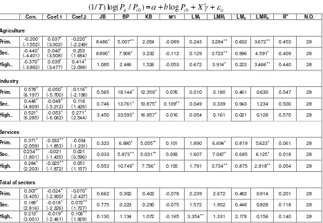
[image:5.595.72.539.193.516.2]

Table 5 presents a series of estimates for conditional sector productivity convergence, with the level of schooling as a proxy for human capital (NUTs III). Three levels of schooling were considered (primary, secondary and higher education) represented by different variables. These variables were obtained through the percentage of the population with each level of schooling in relation to the total number of people, taking into account the data from the Census 2001. Different estimates for each sector were carried out for level of schooling so as to avoid problems of multicollinearity.

Table 5: Empirical evidence of the importance of the level of schooling in the convergence of productivity in the various economic sectors

it i

i

it

P

b

P

X

P

T

)

log(

/

0

)







log

0











/

1 (

Con. Coef.1 Coef.2 JB BP KB M’I LMl LMRl LMe LMRe R2 N.O.

Agriculture

Prim. -0.200 (-1.552)

0.037* (3.302)

-0.220*

(-2.249) 8.486* 5.007** 2.054 -0.089 0.243 3.284** 0.632 3.672** 0.453 28 Sec. -0.440*

(-4.401) 0.040* (3.508)

0.253

(1.684) 8.890* 7.908* 3.232 -0.112 0.129 3.723** 0.996 4.591* 0.409 28 High.. -0.370*

(-3.882) 0.039* (3.477)

0.414*

(2.098) 1.085 2.466 1.526 -0.053 0.672 3.914* 0.223 3.466** 0.440 28

Industry

Prim. 0.578* (6.197)

-0.050* (-5.700)

-0.116*

(-2.198) 0.565 18.144* 12.359* 0.076 0.010 0.180 0.461 0.630 0.547 28 Sec. 0.448*

(4.809)

-0.048* (-5.212)

0.118

(1.426) 0.746 13.761* 10.875* 0.109** 0.049 0.339 0.943 1.234 0.500 28 High.. 0.521*

(6.285)

-0.053* (-6.062)

0.271*

(2.544) 3.450 33.593* 16.957* 0.016 0.054 0.161 0.021 0.128 0.570 28

Services

Prim. 0.371* (2.059)

-0.032** (-1.853)

-0.034

(-1.231) 0.323 6.990* 5.055** 0.101 1.890 6.694* 0.819 5.623* 0.061 28 Sec. 0.234**

(1.801) -0.021 (-1.435)

0.021

(0.596) 0.033 5.873** 5.031** 0.093 1.607 7.047* 0.685 6.125* 0.018 28 High. 0.284*

(2.203)

-0.025** (-1.872)

0.051

(1.157) 0.553 10.749* 7.736* 0.105 1.791 3.734** 0.875 2.818** 0.054 28

Total of sectors

Prim. 0.307* (3.405)

-0.024* (-2.900)

-0.070*

(-2.427) 0.662 0.302 0.402 -0.078 2.239 2.672 0.482 0.914 0.201 28 Sec. 0.188*

(2.816)

-0.018* (-2.326)

0.072**

(1.727) 0.775 0.223 0.290 -0.075 1.572 1.952 0.448 0.828 0.118 28 High.. 0.213*

(3.001)

-0.019* (-2.461)

0.106**

(1.929) 0.130 1.134 1.072 -0.165 3.354** 1.331 2.178 0.156 0.140 28

Note: Prim., estimate with primary education; Sec., estimate with secondary education; High., estimate with higher education; Con., constant; Coef.1, coefficient of convergence; Coef. 2 coefficient of level of schooling; JB, Jarque-Bera

test; BP, Breusch-Pagan test; KB, Koenker-Bassett test: M’I, Moran’s I; LMl, LM test for spatial lag component”; LMRl,

robust LM test for spatial lag component; LMe, LM test for spatial error component; LMRe, robust LM test for spatial

error component; R2_{, r squared adjusted; N.O., number of observations *, statistically significant to 5%; **, statistically}

significant to 10%.

In agriculture, for the three levels of schooling, the indications of divergence are maintained, since the coefficients for convergence present a positive sign with statistical significance, although the values are slightly lower, which is a sign that the level of schooling productivity convergence in this sector, albeit slightly. On the other hand, as could be expected, primary education has a negative effect on the growth of productivity in agriculture for the period 1995 to 2002, while higher education has a positive effect. Therefore, the progress in the level of schooling in this sector improves productivity performances. As far as the LM test of specification are concerned, with the exception of the results obtained from the estimations of higher education, all figures confirm the previous results for this sector, or, in other words, the better specification of the model is with the spatial error component.

Industry confirms in these estimations the signs of productivity convergence across the NUTs III of mainland Portugal from 1995 to 2002, a fact which is only favoured by higher education (since the effect of higher education is positive and increases convergence). The non-existence of indications of spatial autocorrelation was also confirmed, given the values of the LM tests.

(6)

associated to the variables of the level of schooling has statistical significance). On the other hand, taking into account the LM tests, it is confirmed that the better specification of the model is with the spatial lag component.

In the total of sectors, something similar to what was verified in services can see, or, in other words, the convergence coefficient has no statistical significance in the estimations for absolute convergence, but is present in the estimations for conditional productivity convergence with human capital. The difference is that here the coefficients of conditioning variables demonstrate statistical significance, an indicator that convergence in the total of sector sis conditioned by level of schooling.

Finally, it should be noted that the greatest marginal effect is through higher education schooling, which indicates that the higher the level of schooling, the greater the growth in productivity.

5. EMPIRICAL EVIDENCE OF CONDITIONAL CONVERGENCE WITH SPATIAL EFFECTS AND CROSS-SECTION DATA, AT PARISH LEVEL

The results concerning OLS estimates of conditional convergence with tests of spatial specification are present in Table 6, which follows ((7)Martinho, 2011c).

Table 6: OLS estimation results for the equation of absolute convergence with spatial specification tests

it i i

it

P

b

P

T

)

log(

/

0

)







log

0





/

1 (

Constant Coef. b JB BP KB M’I LMl LMRl LMe LMRe

_

R

2 N.O.

-0.052* (-16.333)

0,001* (15.639)

1.819 1.012 1.052 3.074* 92.164* 3.764* 187.805* 98.405* 0.567 4050

Note: JB, Jarque-Bera test; BP, Breusch-Pagan test; KB, Koenker-Bassett test: M’I, Moran’s I; LMl, LM test for spatial

lag component; LMRl, robust LM test for spatial lag component; LMe, LM test for spatial error component; LMRe, robust

LM test for spatial error component;R2, coefficient of adjusted determination; N.O., number of observations; *,

statistically significant to 5%; **, statistically significant to 10%.

The product diverged in Portugal between 1991 and 2001. There are not indications of heteroskedasticity, according to the BP and KB tests. Convergence/divergence in the product will be conditioned by spillover and spatial error effects according to the LM tests.

Table 7 presents the results of the estimates of spillover and spatial error effects.

Table 7: ML estimation results for the equation of conditional convergence with spatial effects

it i it

ij i

it

P

W

p

b

P

T

)

log(

/

₀

)











log

₀





/

1 (

Constant Coefficient _coefficientSpatial Breusch-Pagan

_R

_ 2 N.Observations

-0.267 (-0.978)

0.001* (10.227)

0.990* (150.612)

1.958 0.653 4050

Note: *, statistically significant to 5%; **, statistically significant to 10%; ***, spatial coefficient of the spatial error model.

The convergence coefficient are more or less the same, but the spatial coefficient confirm the existence of spatial autocorrelation.

6. CONCLUSIONS

At NUTs III level and with panel data, we find some signs of convergence essentially in the industry. At NUTs III level and with cross-section data, it can be seen that sector by sector the tendency for productivity convergence is greatest in industry. With reference to spatial autocorrelation it is also confirmed that this possibly exists in agriculture and services, when taking into account the LM tests. Following the procedures of Florax et al. (2003) the equation is estimated with the spatial error component for agriculture and the spatial lag component for services, and it can be seen that the consideration of these spatial effects does not significantly alter the results obtained previously with the OLS estimation. The level of schooling as proxy for human capital conditioning productivity convergence, improves the value and the statistical significance of convergence coefficients. On the other hand, above all the variable which represents higher education shows indications which directly favour the growth of productivity, since the coefficient associated to it presents in all economic sectors the greatest marginal positive effect.

At the parish level, it can be seen that product is subject to positive spatial autocorrelation and that the product diverged between 1991 and 2001 in Portugal. This is a preoccupant situation, because we are the population all in the littoral and no people in the interior.

(7)

7. REFERENCES

1. N. Islam. Growth Empirics : A Panel Data Approach. Quarterly Journal of Economics, 110, 1127-1170 (1995). 2. R. Solow. A Contribution to the Theory of Economic Growth. Quarterly Journal of Economics (1956).

3. V.J.P.D. Martinho. Sectoral convergence in output per worker between Portuguese regions. MPRA Paper 32269, University Library of Munich, Germany (2011a).

4. X. Sala-i-Martin. Regional cohesion: Evidence and theories of regional growth and convergence. European Economic Review, 40, 1325-1352 (1996).

5. V.J.P.D. Martinho. Spatial effects and convergence theory in the Portuguese situation. MPRA Paper 32185, University Library of Munich, Germany (2011b).

6. R.J.G.M. Florax; H. Folmer; and S.J. Rey. Specification searches in spatial econometrics: the relevance of Hendry´s methodology. ERSA Conference, Porto 2003.