Munich Personal RePEc Archive
Life-Cycle Consumption: Can Single
Agent Models Get it Right?
Bick, Alexander and Choi, Sekyu
Goethe University Frankfurt, Universitat Autònoma de Barcelona
February 2011
Life-Cycle Consumption:
Can Single Agent Models Get it Right?
Alexander Bick
Goethe University Frankfurt
Sekyu Choi
Universitat Aut`onoma de Barcelona∗
February 2011
[PRELIMINARY]
Abstract
In the quantitative macro literature, single agent models are heavily used to explain “per-adult equivalent” household data. In this paper, we study differences between consumption predictions from a single agent model and “adult equivalent” consumption predictions from a model where household size evolves deterministically over the life-cycle and affects individual preferences for consumption. Using a theoretical model we prove that, under mild conditions, these predictions are different. In particular, the single household model cannot explain patterns in life-cycle consumption profiles (the so called ’humps’), nor cross sectional inequality in consumption orig-inating from the second model, even after controlling for household size using equivalence scales. Through a quantitative exercise, we then document that differences in predictions can be sub-stantial: total (per-adult equivalent) consumption over the life-cycle can be up to 5% different, depending on the specific parameterization. We find a similar number for total cross sectional inequality.
Keywords: Consumption, Life-Cycle Models, Households
JEL classification: D12, D91, E21, J10
∗email: [email protected] and [email protected]. We thank Dirk Krueger, Jose-V´ıctor R´ıos-Rull,
1
Introduction
To understand life-cycle consumption, economists seem to have converged to single agent
mod-els, given their tractability and ease of use. In the quantitative macroeconomic literature, a standard
approach entails extracting “per-adult equivalent” (or equivalized) consumption facts from
house-hold survey data and use it as a target to be replicated by single agent models, which are calibrated
using also equivalized household income. Some papers in this vein includeKrueger and Perri(2006),
Blundell et al. (2008), Kaplan and Violante(2009) and Guvenen and Smith(2010).1
However, this approach faces the inherent challenge that consumption decisions might depend
on household size and composition through non trivial channels. In this paper we ask about the
differences between the predictions of a single agent model and the equivalized predictions of a
model with household size and composition effects. Specifically, we are interested in predictions
from the standard incomplete markets model for mean and cross sectional inequality of life-cycle
consumption.
We perform our analysis by extending this framework to allow for deterministic changes in
household size and composition during the life-cycle. Moreover, we let these changes affect optimal
decisions on consumption and savings in a unitary model approach similar toAttanasio et al.(1999)
and Gourinchas and Parker(2002). While these studies use a general “taste shifter” depending on
household size and composition, we propose an explicit formulation combining (i) equivalence scales,
which reflect economies of scale in household consumption and (ii) utility weights, which make
ex-plicit the value of having a household of different sizes and compositions. This setup accommodates
both the case of single households (theSinglemodel) and the case where household size varies
dur-ing the life-cycle (theDemographicsmodel). Obviously, we can have as manyDemographicsmodels
as combinations between equivalence scales and utility weights.
Using this framework, we study differences between the predictions of the Single model,
cali-brated using equivalized household income, and the equivalized household consumption from the
Demographics model (which uses total household income). Given that the Single model is just a
1
particular case of what we label theDemographicsmodel, we think of this framework as the mildest
test to the single household approach.
Throughout our analysis, we rely on equivalence scales to transform household data into “adult
equivalent” data. These scales are functions of household size and composition and typically used
to deflate total household information (like consumption and income) by a number less than than
the actual household size, in order to allow for economies of scale inside the household. This
approach has gained importance in the macro literature: in the 2010 special issue of the Review of
Economic Dynamics, equivalence scales are used to obtain consistent “individual” cross sectional
facts for a wide range of countries.2 Another example isFern´andez-Villaverde and Krueger(2007),
who discuss the properties of different types of equivalence scales and their effect on life-cycle
consumption profiles.3
Our quantitative results show that the differences between equivalized consumption data from
theDemographicsmodel and individual data from theSinglemodel can be substantial, both in terms
of predicted levels and cross sectional inequality. The differences are increasing in the difference
between utility weights (the extra utility households derive from consuming in a household with
additional members) and the value of the equivalence scales. Intuitively, the larger this difference,
the larger the motives for households in theDemographicsmodel to allocate consumption in periods
where household size is larger: the utility of doing so gains importance relative to the penalization
in terms of the cost of sharing. Hence, the differences in predictions with respect to theSinglemodel
are going to be high since there equivalization has only an effect through the calibrated individual
income profile. Furthermore, differences in these predictions depend on the stage of the life cycle:
when preferences for household size are high (low), equivalized consumption from Demographics
model can be up to 15% (5%) higher (lower) than in the Singlemodel when household size peaks
(around age 35).
Since we are the first to consider (to the best of our knowledge) the notion of utility weights in
theDemographics model, there is no direct evidence of their value in the literature so we perform
2
SeeKrueger et al.(2010) for a general description andHeathcote et al.(2010) for the US economy.
3
our analysis considering a variety of cases. Nevertheless, using estimates from Attanasio et al.
(1999) we can compute the value of the implied utility weights, under specific equivalence scales.
We find that the empirical evidence inAttanasio et al.(1999) falls in our considered ranges for the
utility weights and suggests that in most cases utility weights are larger than equivalence scales.
The structure of the paper is as follows. In Section 2 we discuss our proposed preferences for
the household and Section3 we present theoretical predictions in a stylized two period framework.
Sections2and5discuss the model we use to quantify these theoretical predictions. In Section6we
discuss the quantitative features of the model and the calibration strategy while Section 7 shows
our main quantitative results. In the last section we present our conclusions and extensions of our
exercise.
2
Demographics and Preferences
We follow Attanasio et al. (1999) andGourinchas and Parker (2002) and introduce exogenous
and deterministic demographics via a taste shifter into the standard life-cycle model:
U(c, Nad, Nch) = exp(ξ1Nad+ξ2Nch)u(c), (1)
with Nad being the number of adults and Nch the number children in the household. In the
subsequent analysis we will use an explicit formulation of the taste shifter:
u(c, Nad, Nch) =δ(Nad, Nch)u
c φ(Nad, Nch)
. (2)
Household utility U(c, Nad, Nch) is the product of the utility from adult equivalized consumption
u c φ(Nad,Nch)
, where φ(Nad,t, Nch,t) transforms total household consumption into an adult
equiv-alent consumption, and the utility weight δ(Nad, Nch) which differs across households of different
size and composition. We are not the first to use such an explicit formulation of the taste shifter.
Fuchs-Sch¨undeln (2008) setsδ equal toφwhich are then both a function of the average household
size and an equivalence scale. In contrast, Hong and R´ıos-Rull (2007) set δ = 1 to one and
esti-mate the equivalence scale φfor different household size. Both papers do not provide any further
In the theoretical part of this paper, we will not rely on any specific functional form of φ. In
general we might think of it as prototypical equivalence scale which are calculated with information
on expenditure shares of households. As a concrete example consider the OECD equivalence scale:
φOECD = 1 + 0.7(Nad−1) + 0.5Nch. (3)
According to Equation (3) it takes 1.7$ to generate the same level of welfare out of consumption
for a two adult household that 1$ achieves for a single member household. The three mechanisms
through which household size affects the intra-temporal rate of transformation between
expendi-tures and services are family/public goods, economies of scale, and complementarities, see e.g.
Lazear and Michael (1980). Note that while in Equation (3) each additional adult and child
in-creases the equivalence scale by a constant number, these weights could also vary with household
size and composition. Alternatively, φ could also be obtained from the coefficients on household
size and composition dummies from a regression of consumption on various controls, as discussed
in the introduction.
To also give a hypothetical example to the utility weightδ(Nad,t, Nch,t), which assigns a different
value to the household utility of equivalized consumption across households of different size and
composition, we could be specified in analogy to the OECD equivalence scale (Equation
refequiva-lence scale oecd):
δ(Nad, Nch) = 1 +ωad(Nad−1) +ωchNch. (4)
The first adult has a utility weight of one whereas any further adult and child have the utility
weights ωad and ωad. As with the equivalence scales the weights ω may vary with household size
and composition.
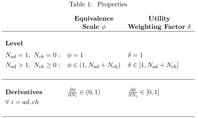
Fern´andez-Villaverde and Krueger (2007) provide a list of six representative estimated
house-hold equivalence scales with properties being summarized in column one of Table 1. To the best
of our knowledge, there is no empirical evidence on the utility weighting factor. As already
men-tioned Fuchs-Sch¨undeln (2008) sets δ = φ whereas Hong and R´ıos-Rull (2007) set δ = 1 for all
household types. Using the same utility function as Attanasio et al. (1999) and their empirical
estimates, δ can be backed out for a given equivalence scale φ. Given the analogy to
Table 1: Properties
Equivalence Utility Scale φ Weighting Factor δ
Level
Nad = 1, Nch= 0 : φ= 1 δ= 1
Nad >1, Nch≥0 : φ∈(1, Nad+Nch) δ∈[1, Nad+Nch]
Derivatives ∂N∂φ
i ∈(0,1)
∂δ
∂Ni ∈[0,1]
∀ i=ad, ch
assumed in Hong and R´ıos-Rull (2007) the utility weighting factor may remain constant as the
household increases, i.e.δ = 1∀Nad, Nch, whereas equivalence scales always increase. On the other
hand an additional household member could also increase the utility weighting factor by one, i.e.
δ =Nad+Nch, whereas equivalence scales always increase by less than one. These properties are
outlined in column 2 of Table 1. Note that our subsequent analysis does not rely on the utility
weight δ and the equivalence scale φ being only a function of the number of adults and children
in a household. We could make them easily dependent on finer categories, as e.g. the number of
children by different age groups. We just stick to the previous case as this approach has been
cho-sen by Attanasio et al. (1999) and Gourinchas and Parker (2002) to introduce demographics into
the life-cycle model. In addition, those who clean the empirical income and consumption series
for household size and composition using equivalence scales rather than the regression approach
usually use equivalence scales that only depend on the number of adults and number of children in
the household.
3
A Two Period Model
We take the most simplistic approach to model household size followingAttanasio et al.(1999),
but allowing for a more structural formulation of the utility function as given by Equation (2). In
particular, we assume that the true data is generated by such a model where demographics play a
a model that abstracts from demographics but takes as input income data that is cleaned of family
size effects through the application of an equivalence scale.
3.1 Basic Setup
We will analyze this question using atwo-period model with deterministic demographics. We
consider a household who lives for two periods and changes its size over time. In particular, we
assume that the household size is one in the first period, e.g. a young person living alone, and
larger one in the second period, e.g. a child is born. These assumptions and their implications for
the utility weighting factor δ and an arbitrary equivalence scale φ, both satisfying the properties
outlined in Table 1, can be summarized as follows:
N1= 1 ⇒ δ1 = 1, φ1= 1
N2>1 ⇒ δ2 >1, φ2 >1,
(5)
without restricting the ratio φ2δ2. The household receives an income stream y1 and y2, and can
borrow and save at an interest r which without loss of generality is set to zero. Similarly, the
discount factor is set to one, i.e. from the perspective of period one the utility in period two is not
discounted.
In the subsequent analysis we will label the data-generating process for consumption as the
Demographics model and the one that abstracts from demographics in the utility function as the
Singlemodel.
In theDemographicsmodel, household size (and composition) affect utility as outlined in
Equa-tion (2) and the available resources for consumption are given by household income such that the
optimization problem is represented by
max c1,D,c2,D
U =u(c1,D) +δ2u
c2,D
φ2
(6)
subject to
c1,D+c2,D=y1+y2≡YD. (7)
avail-able resources for consumption are given by equivalized income. The corresponding optimization
problem is thus
max c1,S,c2,S
U =u(c1,S) +u(c2,S) (8)
subject to
c1,S+c2,S =y1+
y2
φ2 ≡
YS. (9)
In both models the natural borrowing constraint is imposed and the same utility function is used.4
Furthermore, in both specifications equivalized consumption is the unit over which households
optimize which makes the setups comparable. For the Single model the consumption levels c1,S and c2,S in fact reflect equivalized consumption because income as an input to the optimization problem has been equivalized before. For theDemographicsmodel it is obvious in the second period
as the household receives the utility from equivalized consumption c2,D
φ2 which is however also true
in the first period because household size is one in period one such that c1,D = c1φ1,D.
Result 1. The equivalized consumption profile in the Demographics model and Single model only
coincide ifδ2=φ2.
This result can be immediately read of from the two Euler equations which for theDemographics
model is given by
u′(c1,D) =
δ2
φ2
u′
c2,D
φ2
⇔ u′(c1,D) =
δ2
φ2
u′
a2,D
φ2
+ y2
φ2
, (10)
with a2,D = y1−c1,D being the assets carried over from period one. The Euler equation for the
Singlemodel is
u′(c1,S) =u′(c2,S) ⇔ u′(c1,S) =u′
a1,S−
y2
φ2
, (11)
with a2,S =y1+c1,S being the assets carried over from period one. Equation (11) predicts a flat equivalized consumption profile for the Single model. The equivalized consumption profile in the
Demographics model is only flat if δ2 = φ2. If δ2 > φ2, the equivalized consumption profile is
upward sloping, i.e.c1,D = c1,D
φ1 < c2,D
φ2 ,while the opposite is true forδ2 < φ2. In theDemographics model the benefit of consuming one additional unit consumption in the second period
4
The utility function exhibits the standard properties regarding curvature, i.e.u′
(c)>0,u′′
(c)<0 andu(c)′′′ >0, and satisfies the Inada conditions, i.e.u′
(c)
c→0
=∞andu′
(c)
c→∞
1. is associated with the marginal utility of equivalized consumption in period one hu′c2,D
φ2
i
2. which accrues to all household members reflected through the utility weight factor [δ2]
3. has to be divided by the equivalence scale [φ2] because each household member does not get
the full unit to consume but only the fraction φ21 .
Put differently, δ2 provides an incentive to save because the household enjoys a larger utility
from consuming in the second period, as each unit of equivalized consumption is enjoyed by more
(weighted) individuals. However, in period two every unit of consumption has to be shared with
more people which is reflected through the division with the equivalence scale φ2. This reduces
the incentive to save, i.e. to consume the assets, in period two. If δ2 = φ2, the latter two effects
cancel out and therefore equivalized consumption in period one equals equivalized consumption in
period two. If δ2 > φ2, equivalized consumption in period two exceeds equivalized consumption in
period one. Relative to period one, the absolute loss in consumption in period two through the
equivalization is in this case outweighed by the larger gain in household utility through the utility
weight.
Interestingly, such a configuration provides an additional explanation for the hump observed in
equalized consumption documented in Fern´andez-Villaverde and Krueger(2007).
Result 2. Life-time equivalized consumption in the Demographics model only coincides with
life-time equivalized consumption in the Single model, if in the Demographics model the share of
household consumption allocated to period two equals the share of household income received in
period two.
In order to show Result 2, it is helpful to define some variables. First, define on the household
level prior to any equivalization the share of household income y2 received in period two relative
to life-time household income as
η = y2
y1+y2
= y2
YD
. (12)
Second, for theDemographics model define similarly the share of household consumption allocated
to period one relative to life-time household consumption
ζD =
c2,D
c1,D+c2,D
which is of course an endogenous object. Using these expressions life-time equivalized consumption
from the Demographics model can be written as
CD =cD,1+
c2,D
φ2
=
(1−ζD) +
ζD
φ2
(y1+y2) =
(1−ζD) +
ζD
φ2
YD (14)
and life-time equivalized income YS from the Singlemodel as
YS =y1+
y2
φ2
=
(1−η) + η
φ2
(y1+y2) =
(1−η) + η
φ2
YD. (15)
By the budget constraint (9) life-time equivalized consumption from the Single model (CS =
c1,S +c2,S) equals YS. Hence, the difference in life-time equivalized consumption between the
Demographics and the Singlemodel is given by
CD−CS=CD−YS = (η−ζD)
φ2−1
φ2
YD (16)
which proofs Result 2. Whenever η > ζD, the life-time equivalized consumption under the
Demo-graphicsmodel is larger than under the Singlemodel. The opposite is true for η < ζD.
The intuition for this result can be explained best with a concrete example. Assume that the
household income is zero in the first period (y1 = 0), and positive in the second period (y2 >0)
which implies that η= 1. In this case life-time equivalized income in theSinglemodel is y2φ2 which
by the budget constraint equals life-time equivalized consumption. In the Demographics model
in turn, the household has the income y2 available for consumption. By the Inada condition the
household will consume in period one as well such thatc2,D< y2 and thusζD < η = 1. Given that household size is one in period one, in the calculation of life-time equivalized consumption in the
Demographics model the equivalization matters only for period two consumption. Sincec2,D < y2,
“less” in absolute terms is lost through the equivalization in the calculation of life-time equivalized
consumption in the Demographics model compared to the Single model.5 Essentially, Result 2 is
5
More formally, rewrite life-time equivalized consumption in theDemographicsmodel as
CD=c1,D+
c2,D
φ2
= (y2−c2,D) +
c2,D
φ2
=y2−
φ2−1
φ2
c2,D,
which implies becausec2,D< y2 that
CD=y2−
φ2−1
φ2
c2,D> y2−
φ2−1
φ2
y2=
y2
φ2
the implication of a pure accounting exercise. The key driving force behind is that the households
can shift consumption between periods but not income. If income and consumption allocations are
not fully synchronized, then equivalization drives a wedge between equivalized consumption in the
Demographics model and equivalized income.
Note that Result 2 and its derivation are completely independent of the relationship between
δ2 and φ2. These two functions of household size do however determineζD and thus for a given η the relationship between the two equivalized consumption levels.
3.2 Income Inequality
In the following paragraph we introduce income heterogeneity, but not uncertainty, to
demon-strate that the level differences between the two models also translate into equivalized consumption
inequality differences. We will assume that the the economy is populated with a mass of households
of size one, where 12 receives life-time household income YA and the other 12 life-time household incomeYB.
Result 3. Assume that life-time household income differs, i.e.YA
D 6=YDB, but the share of household
income in period two from life-time household income is the same, i.e. ηA=ηB. In this case any
differences in life-time equivalized income between the Demographics and Single model (see Result
2) translate into differences in the level of life-time equivalized consumption inequality.
Setting YDA = 1 and YDB = π with π > 1, it is straightforward to show that the variances of
life-time equivalized consumption in the two models are given by
Var(CS) =
π−1
2 C
A S
2
and Var(CD) =
π−1
2 C
A D
2
. (17)
Hence, the relationship between the two can be summarized as
Var(CS) Var(CD)
=
CA S
CA D
2
. (18)
Whenever life-time equivalized consumption differs between the two models, i.e. η 6=ζD, the level
thusCA
S < CDA, life-time equivalized consumption inequality is larger in the Demographics model. Through the equivalization the absolute loss in equivalized income in theSinglemodel is larger than
the absolute loss in consumption in the Demographics model which reduces life-time equivalized
consumption inequality more in the Singlemodel.
3.3 Income Uncertainty
In the next paragraph, we analyze the role of income uncertainty. Assume there is a mass of
households of size one. In the first period all household have the same income y1 whereas income
may take too values yL
2 < y2H in period two with each state occurring with probability 12. For the
following results it is useful to define period two mean variables as ¯X= 12Pi=L,HXy2=yi
2.
Result 4. In the presence of income uncertainty, the equivalized consumption profile is steeper in
the Demographics model than in the Single model even if δ2 =φ2 and η¯= ¯ζD.
In fact, we will show that Result 4is always true whenever δ2 ≥φ2 and ¯η≥ζ¯D and sometimes even when the inequality operators are reversed. In order to do so it is useful to start with the
first-order condition for the Singlemodel:
u′(c1,S) = 1 2 u′
y1−c1,S+
yL
2
φ2
| {z }
cL2,S
+u′
y1−c1,S +
yH
2
φ2
| {z }
cH2,S
| {z }
ΓS
. (19)
Given the assumptions on the utility function (u′ > 0, u′′ < 0 and u′′′ > 0) the introduction
of uncertainty introduces the standard precautionary savings motive which generates an upward
sloping average consumption profile. The result is standard and induced by Jensen’s inequality.6
6
The easiest way to illustrate this is by settingyL
2 = (1−ǫ)y1φ2andyL2 = (1+ǫ)y1φ2. In the absence of uncertainty,
the natural borrowing constraint induces a flat consumption profile for theSinglemodel. Now assume the household would choose current consumption such that the expected, or ex post the average, consumption profile is flat, i.e.c1 =E1(c2) = 12
h
y1+E
y2
φ2
i
=y1.By Jensen’s inequality, the left hand side of Equation (19) is smaller than
the right hand side. In order to achieve equalityc1,S has to decrease which generates the upward sloping average
The first-order condition for theDemographics model is given by
u′(c1,D) = 1 2 δ2 φ2 u′
y1−c1,D
φ2 + y L 2 φ2
| {z }
cL2,D
+u′
y1−c1,D
φ2 +y H 2 φ2
| {z }
cH2,D
| {z }
ΓS
(20)
For the moment consider the case of δ2 = φ2. Denote with c∗1,S the consumption allocation that solves Equation (19) for theSinglemodel and setc1,D =c∗1,S. Hence, the savings brought to period two are the same in both models (aD =y1 −c1,D = y1−c∗1,S = aS). However, consuming them in the Demographics model is associated with sharing reflected through the equivalization. As a
consequence the uncertain part of equivalized cash on hand, i.e. equivalized assets plus equivalized
income, is larger in the Demographics model. This implies that in the Demographics household
more savings will be accumulated compared to the Singlemodel and period one consumption will
be lower, i.e. c∗1,D < c∗1,S.7 The difference in period one consumption is increasing in the ratio φ2δ2 and even for values of δ2< φ2, in the presence of uncertaintyc∗1,D may still fall below c∗1,S because of the precautionary savings motive.
From Result2we know that for η≥ζD life-time equivalized consumption in theDemographics
model is at least as large as than in theSinglemodel implying that also in the case with uncertainty
the following relationship has to hold for ¯η≥ζ¯D:
c1,D+ ¯
c2,D
φ2 ≥
c1,S+ ¯c2,S. (21)
As we have already shown forδ2≥φ2 ⇒ c1,D < c1,S Equation (21) thus implies that c2¯φ2,D >c¯2,S. Note that even for values of ¯η <ζ¯, the equivalized consumption profile in theDemographics model
is steeper than in theSinglemodel as long as
¯
η >ζ¯Dξ−
φ2
φ2−1
(ξ−1)
| {z }
<ζ¯D
, (22)
7
More technically, c1,D =c
∗
1,S ⇒ ci
2,D
φ2 < c
i
2,S ∀ i= 1,2 and hence by the properties of the utility function
ΓS>ΓD. Equation (20) can thus only be satisfied if period one consumption is lowered such thatc
∗
1,D < c
∗
with ξ = c1,S
c1,D and ξ > 1. The key message from Result 4 is that the equivalized consumption
profiles do not coincide any longer for the case of δ2 =φ2 and ¯η= ¯ζD.
3.4 Income Inequality and Income Uncertainty
In the previous subsection income heterogeneity/inequality in period two implied by the income
uncertainty
• does not lead to any equivalized consumption inequality in period one as in both models all
agents are the same in period one,
• maps one to one into equivalized consumption inequality in period two as in both models all
agents enter have the same (model-dependent) level of assets.
Result 3 of course applies with respect to life-time equivalized consumption inequality. We now
add to the income uncertainty and thus income heterogeneity in period two, income heterogeneity
in period one. Simply assume that in each model there is a mass of households of size one, with 12 having incomeyL
1 and 12 y1H in period one and y1L< yH1 . The two possible income states in period
2 are as before given byyL
2 and y2H, each occurring with probability 12 independent of the income
realization in period one.
Result 5. The same level of equivalized consumption inequality in period one in the Demographics
andSinglemodel, implies a lower level of consumption inequality in period two in theDemographics
model.
This setup now permits only to make relatively general statements. It can be shown that the
variance of equivalized consumption in period one is
Var(c1,i) = 1 4(c
H
1,i−cL1,i)2 ∀i=S, D, (23)
and in period two for theDemographics model
Var
c2,D
φ2 =1 4 " 1 φ2 2
y1H −y1L−cH1,D−cL1,D2+
yH
2 −yL2
φ2 2# =1 4 " aH D
φ2 −
aH D φ2 2 +
y2H −y2L φ2
and for theSinglemodel
Var (c2,S) = 1 4
"
yH1 −yL1 −cH1,S−cL1,S2+
yH
2 −yL2
φ2
2#
=1 4
"
aHS −aLS2+
yH
2 −yL2
φ2
2#
.
(25)
The key difference is that for a given level of equivalized consumption inequality in period one, i.e.
cH1,D −cL1,D = cH1,S −cL1,S, the difference in equivalized assets in the Demographics model will be smaller than in theSinglemodel which yields a smaller variance. However, the level of consumption
inequality in period one reflects endogenous choices and will be in general different between the
two models. Result 5 demonstrates the non-trivial interactions that the presence of
demograph-ics in preferences has on equivalized consumption inequality relative to a model without such a
dependency.
3.5 Summary
In the absence of income inequality and uncertainty equivalized consumption data generated
by a simple model with demographics can only be replicated with a model without demographics
but using equivalized income under two strict conditions. First, the utility weightδ needs to equal
the equivalence scaleφ. Otherwise, the equivalized consumption profiles are different. Second, the
share of household consumption allocated to period two (ζD) in the model with demographics needs
to equal the share of household income received in period two (η). Otherwise, the level of life-time
equivalized consumption and inequality differ. Once income uncertainty is introduced, even for the
case of δ = φ and η = ζD the Single model cannot replicate the equivalized consumption profile
generated by theDemographics model.
4
CRRA Preferences
In quantitative life-cycle models CRRA preferences are the prevailing choice for the utility
function. In the next paragraph we will discuss the role of the parameter of relative risk aversion
in theDemographics model.
(6) and (7) using CRRA preferences:
max c1,D,c2,D
U = c1,D
1−α 1−α +δ2
c2
,D
φ2
1−α
1−α (26)
subject to
c1,D+c2,D=y1+y2≡YD. (27)
The implied Euler equation for equivalized consumption is
c−α1,D= δ2
φ2
c2,D
φ2
−α
, (28)
In conjecture with the budget constraint, the optimal equivalized consumption can be obtained
c1,D=
1
1 +φ2δ2 1
α φ2
and c2,D
φ2 = δ2 φ2 1 α
1 +φ2δ2 1
α φ2
. (29)
Since CRRA preferences are just a special case of the general utility function discussed before,
we can see here again that it is only the ratio φ2δ2 which determines the profile of the equivalized
consumption. δ2 =φ2 implies a flat profile,δ2 > φ2 a positive slope, whereas the opposite is true
for δ2 < φ2. In the latter two cases, the slope is tilted towards one as α increases. A large α
means a low intertemporal elasticity of substitution and thus a low willingness to have differences
in equivalized consumption between the two periods.
While the profile of equivalized consumption is entirely determined by φ2δ2 1
α
, the profile of
household consumption, i.e. c2,D −c1,D, is in turn determined by
δ2 φ2
1
α
φ2. The household
con-sumption profile is thus only increasing if
α >1− lnδ2 lnφ2
. (30)
Since α is restricted to positive values, condition (30) is always satisfied for δ2 ≥φ2. Any value of
α >1, which includes the typical range of values used for calibration, also satisfies Equation (30)
generate an upward-sloping household consumption profile if δ2 < φ2.
5
Quantitative Model
Our goal here is not to a build quantitative model that is able to replicate all the empirical facts
with respect to consumption. Our aim is to test and evaluate the implications of our theoretical
analysis with a simple, stripped-down version of a standard incomplete markets life-cycle model.
Households start their economic life in periodt0 with zero assets. During their working life until
periodtwthey receive a stochastic incomeytin every period. There is no labor supply choice. From
periodtw+1 onwards households are retired and have to live from their accumulated savings during
working life. We abstract from pensions. Life ends with certainty at ageT and households do not
leave bequests and cannot die with debt. Households have access to a risk-free bondawhich pays
the interest rater. In this version of the paper, households can borrow up to the natural borrowing
constraint (level of debt that they can always repay for sure) at the interest rate r. We leave the
case of a zero borrowing constraint as an extension.
In the Demographics model household size changes over the life-cycle deterministically and is
homogenous across all households. The maximization problem is given by
max
{at+1}T
−1
t=t0
E0
T
X
t=t0
βδtu
ct
φt
subject to (31)
ct+at+1≤(1 +r)at+yt (32)
at+1≥amin,t. (33)
whereδt and φt are functions of household age, household size and composition (t,Nad,t andNch,t
respectively). The income process is given by:
lnyt=̺t+ǫt, (34)
where̺t is an age-dependent experience profile and
The Euler equation to this problem is given by
δt
φt
u′
ct
φt
=β(1 +r)δt+1
φt+1
Et
u′
ct+1
φt+1
. (36)
The structure of the Single problem is very similar. Demographics don’t affect the utility
function while incomeyt is deflated by household size through equivalence scalesφt:
max
{at+1}Tt=−t10
E0
T
X
t=t0
βu(ct) subject to (37)
ct+at+1≤(1 +r)at+
yt
φt
(38)
at+1≥amin,t, (39)
withyt following the same process as described in Equations (34) and (35).
The Euler equation to this problem is given by
u′(ct) =β(1 +r)Et
u′(ct+1). (40)
6
Quantitative Features of the Model
A model period is one year. Agents start life at age 25, retire when 65 and live with certainty
until age 75. In this version of the model, and to maintain maximum comparability with our
theoretical analysis, we set β = 1 and β(1 +r) = 1. We set the CRRA coefficient α equal
to 1.57, the value estimated and used by Attanasio et al. (1999). In the next section, we use
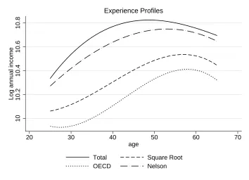
as a benchmark the square root scale φSQRt = √Nad+Nch, and compare our results with the
OECD ad the Nelson scales. These choices follow closely the discussion of equivalence scales in
Fern´andez-Villaverde and Krueger(2007). The OECD scale has the lowest economies of scale while
the opposite is true for the Nelson scale. The square root scale is almost identical to the “Mean”
scale inFern´andez-Villaverde and Krueger (2007) which is their preferred choice.8
As for utility weights, we remain agnostic and compare three extremes: (i) δt = 1 represents
the case when households do not value household size; (ii)δt =Nt=Nad,t+Nch,t is the opposite,
8
since households always enjoy having more members; and (iii) an intermediate case whenδt =φt,
i.e., we let the utility weight take the same value as the equivalence scale.
6.1 Income
We use data from the Current Population Survey, from 1984 to 2003. We use the March
supplements for years 1985 to 2004, given that questions about income are retrospective. We use
total wage income (deflated by CPI-U, leaving amounts in 2000 US dollars), and apply the tax
formula of Gouveia and Strauss(1994) to get after-tax income.9
We define a full time/full year (FTFY) worker, as someone who worked more than 40 hours
per week and more than 40 weeks per year and earned more than $2 per hour. We construct total
household income Wiτ for household iobserved in yearτ, as the sum of individual incomes in the
household for all households with at least one full time/full year worker. Then, we estimate the
following regression:
log
Wiτ
φiτ
=Diτage̺+Xiτγ+ǫiτ (41)
whereφiτ is an equivalence scale,Dageiτ represents a set of age dummies of the head of household,̺
andγ are estimated coefficients andεare estimation errors. Note that for theDemographics model
we use household income for the estimation, i.e. φiτ = 1 ∀ i, τ. We also control for cohort effects
and time effects by introducing birth year and year dummies in Xiτ.10
From this estimation, we are interested in the regression coefficients associated with age
dum-mies of the household head (experience profiles in the model). In our exercise below, we use
smoothed profiles, which we show in Figure1 for different choices of equivalence scales.
From the estimation residuals, we calibrate the income process in (35). Our calibration
pro-cedure is standard and follows Storesletten et al. (2004): we pick values of ρ and σ in order to
9Wage income in the CPS is pre tax income. 10
Since year dummies are perfectly collinear with age and birth cohort dummies, we follow Aguiar and Hurst (2009) and include normalized year dummies instead, such that for each yearτ
X
τ
γτ = 0 and
X
τ
τ γτ = 0
where {γτ}are the coefficients associated to these normalized year dummies. To compare life-cycle profiles across
Figure 1: Experience Profile for Households
10
10.2
10.4
10.6
10.8
Log annual income
20 30 40 50 60 70
age
Total Square Root
OECD Nelson
Experience Profiles
Figure 2: Profiles for Household Size and Composition
1
1.5
2
2.5
3
25 30 35 40 45 50 55 60 65 70 75
Age
[image:21.612.130.482.432.687.2]Table 2: Calibrated Parameters: ρ,σ and σ0
ρ σ σ0
0.9906 0.0189 0.1575
minimize the square difference between the profile of observed cross-sectional variances of income
and the simulated one (given the chosen parameters). We also pick values of σ0, the standard
deviation for the unconditional distribution of the first income shockε0 in order to match the cross
sectional variance of income for our first age group (25 years old). We present these values in table
2. We discretize this calibrated process using the Rouwenhorst method, using 20 points for the
shock space. This methodology is specially suited for our case, given the high persistence of the
process. This is discussed in Kopecky and Suen(2010).
To maintain full comparability with our simple theoretical model, we perform anex-post
equiv-alization procedure for the income process in theSinglemodel: we use the same calibrated income
profiles and shocks in both the Demographics and Single models (the calibration in Figure 1 and
Table 2) and then feed the equivalized experience profiles to theSinglemodel. Besides making the
quantitative model more comparable to the theoretical model, this approach maintains the same
shock structure across considered equivalence scales, making the comparison of biases more direct,
since no extra “noise” is being introduced by different volatility parameters. This would be the
case for an alternative approach, or an ex-ante equivalization: estimating Equation (41) with a
particular equivalence scale φiτ, resulting in different age profiles and calibrated income shocks for
theSinglemodel. Since the income has already been equivalizedex-ante, there is no need to do so
in budget constraint (38).11
6.2 Family Structure
We use the March supplements of the CPS for years 1984 to 2003. For each household, we
count the number of adults (individuals age 17+) and the number of children: individuals age 16
or less who are identified as being the “child” of an adult in the household. We restrict our sample
to consider households with at most 2 adults and 4 children. We compute two separate profiles:
one for number of adults and one for number of children. As above, we run dummy regressions to
11
extract life-cycle profiles, where the considered age is that of the head (irrespective of gender) and
control for cohort and year effects. After extracting these life-cycle profiles, we smooth them using
a cubic polynomial in age, and restrict the number of children to zero after age 60. The results of
this procedure are in Figure 2.
7
Results
7.1 Deterministic Framework
We first present a deterministic version of the model, to highlight intuition and draw
compar-isons with the theoretical results in the previous section. Since there is no heterogeneity for any
given age, in this subsection we present results on mean consumption profiles only.
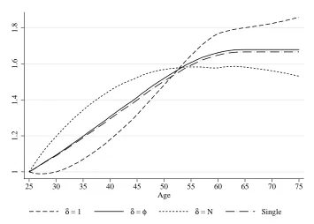
7.1.1 Household Consumption
Figure 3shows household consumption for different cases of household preferences, normalized
at age 25. As a benchmark we also add the profile for theSinglemodel. Recall that the output of
theSinglemodel is an equivalized profile which is flat, sinceβ(1 +r) = 1. For the different cases of
the Demographics model, consumption profiles exactly replicate the profile of household size and
peak exactly when household size is the largest (see Figure2). Recall from the discussion in Section
4that for any ratio of φδ the household consumption profile is increasing in household size ifα >1.
For the case when δt = Nt (utility weight equals total household size) the household values its
size the most and accordingly the mean household consumption profile exhibits the largest “hump”
early in life and the fastest decrease later in life. The opposite is true for the utility weight δt= 1:
households do not enjoy extra utility when its size grows, so we get the flattest consumption profile
earlier in life and the slowest decline later, among all utility weight cases. Finally, δt = φt is an
intermediate case since in general,φt∈[1, N]. As seen from Figure3, the profile for total household
consumption for this case lies exactly in between the two cases above.
All profiles intersect around age 50, which is the result of household size being equal at both
that age and age 25 (first period of the model). Given the assumption of a natural borrowing
constraint and no income uncertainty, periods with the same household size lead in all cases to
Figure 3: Household Consumption Relative to Age 25
.6
.8
1
1.2
1.4
25 30 35 40 45 50 55 60 65 70 75
Age
δ = 1 δ = φ δ = N Single
Note: Deterministic Income; Square Root Scale
Figure 4: Equivalized Consumption Relative to SingleModel
.9
1
1.1
1.2
25 30 35 40 45 50 55 60 65 70 75
Age
δ = 1 δ = φ δ = N
[image:24.612.132.481.411.675.2]looking at the Euler equation (36) for the deterministic case, and substituting forward, it is clear
that whenever two periods have the same household size, total consumption is the same, no matter
what the utility weight is (again, using the fact that β(1 +r) = 1).
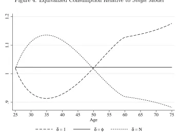
7.1.2 Equivalized Consumption
In Figure4, we show equivalized consumption profiles from theDemographics model relative to
theSinglemodel.12 We see that for every case ofδt, equivalized consumption from theDemographics
model does not coincide with the predictions of the Single model. Just as predicted by Result 1,
the equivalized consumption profile generated by the Demographics model has the same shape as
the one generated by the Single model if δt = φt. Whenever δt > φt, equivalized consumption is
increasing in household size and the opposite is true forδt< φt. Even in the case where the utility
weight is equal to the chosen equivalence scale (δt=φt) we get a biased profile of adult equivalent
consumption: the equivalized consumption from the Demographics model is around 2.2% higher
than in the single model on average (and in terms of lifetime equivalized consumption). The same
happens in the case with δt = 1 and δt =Nt, with lifetime differences of equivalized consumption
relative to the Single model around 3.5% and 1.0% respectively. This fact can be explained with
Result 2 from the previous section: only when shares of household consumption and household
income in each period and across models are the same, the level of equivalized consumption will
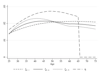
be the same.13 That this condition is not met can be clearly seen in Figure 5, where we show that
shares of household consumption per age over lifetime household consumption are equal across
models only at age 25 and age 50; in terms of household income, the shares are all the same across
models (by construction) but very different to the consumption shares at all ages.
7.2 Stochastic Framework
We now show simulation results from a model with the stochastic income process described in
the previous section. We want to analyze simulated profiles of mean equivalized consumption, the
12
Note that because theSinglemodel predicts a flat consumption profile, theDemographicsprofiles relative to age 25 look exactly the same except of a level shift.
13
In fact, in the multi-period case, also other combinations of household consumption shares could generate a life-time equivalized consumption in the Demographics model that coincides with the Single model as long as
PT
t=t0
ζt,D
φ2 =
PT
t=t0
ηt
φt with
PT
t=t0xt= 1∀x=ζD, η. The Demographicsmodel would however have to generate
Figure 5: Household Consumption and Income Shares
0
.01
.02
.03
25 30 35 40 45 50 55 60 65 70 75
Age
ζδ = 1 ζδ = φ ζδ = N η
Note: Deterministic Income; Square Root Scale
associated implications for equivalized consumption inequality over the life-cycle and the differences
between theDemographics approach and the Singlemodel.
7.2.1 Equivalized Consumption Means
Figure 6 shows the effect of uncertainty on the profile of mean equivalized consumption across
different models relative to the respective consumption at age 25. Note that this figure is not the
counterpart to Figure3which showed household consumption. As discussed in the context of Result
4, in theSinglemodel consumption is increasing in age, reflecting the role of precautionary savings.
This is true also for the rest of the models and in stark contrast to the deterministic case where
theSinglemodel profile was completely flat. The effect of utility weights is also present here: when
δt= 1, there is no utility from household size, hence the household consumes more when household
size is low (later ages); moreover, consumption growth mirrors negatively the growth in household
size. In the model with a deterministic income, equivalized consumption followed household size
for δt =Nt. In the presence of income uncertainty, the precautionary savings motive is stronger
Figure 6: Equivalized Consumption Relative to Age 25
1
1.2
1.4
1.6
1.8
25 30 35 40 45 50 55 60 65 70 75
Age
δ = 1 δ = φ δ = N Single
Note: Stochastic Income; Square Root Scale
Figure 7: Equivalized Consumption Relative to SingleModel
.95
1
1.05
1.1
1.15
25 30 35 40 45 50 55 60 65 70 75
Age
δ = 1 δ = φ δ = N
[image:27.612.131.481.419.672.2]it is positive until retirement, and has the steepest slope when household size increases. When
household size starts to decrease, this slope starts decreasing as well. For the intermediate case
(δt = φt), equivalized consumption tracks very closely the single household case, but the slope
of the profile is marginally steeper. The latter effect is predicted by Result 4 and can be seen
even more clearly in Figure 7 where we present equivalized household consumption for the three
Demographics models, relative to the single household model prediction. All the relative effects we
saw in the deterministic case remain the same. On the other hand, average equivalized consumption
relative to the single household model is 4.8%, 3.7% and 2.7% larger over the lifetime for the cases
with δt = 1, δt = φt and δt = Nt respectively. These values are higher than in the deterministic
case because of the different allocation of consumption over the life-cycle, compare Figures 5 and
8. Via this channel, the introduction of uncertainty increases the relative differences between the
predictions ofDemographics andSingle models, all else constant.
7.2.2 Equivalized Consumption Inequality
With the introduction of stochastic income processes, we can compare equivalized consumption
inequality for our different models over the life-cycle. In Figure 9 we see that all models imply
increasing equivalized consumption inequality in the life cycle. However, how inequality evolves
depends again on the choice of utility weights. For the case whenδt=Nt, equivalized consumption
is higher when the household is larger (earlier in life), so equivalized consumption tracks income
shocks more closely which can also be seen in Figure8. Hence, the cross sectional inequality related
to that model rises the fastest until around age 50. On the other hand, whenδt= 1 and households
do not enjoy household size, households want to postpone consumption to periods when household
size is small; hence, they accumulate more assets for every income shock, relative to the δt =Nt
case. Hence, cross sectional consumption inequality is lower earlier in life for the δt = 1 setup in
comparison to when δt =Nt. Later in life, there is a reversion of absolute levels of consumption
inequality, since households in theδt= 1 economy have accumulated assets in a more heterogeneous
way, which leads to more heterogeneous consumption. The opposite is true for theδt = 1 case, so
the lines in the figure change their relative position.
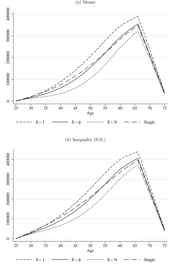
In Figure 10 we show the evolution of equivalized assets and cross section inequality (standard
Figure 8: Household Consumption and Income Shares
0
.01
.02
.03
25 30 35 40 45 50 55 60 65 70 75
Age
ζδ = 1 ζδ = φ ζδ = N η
Note: Stochastic Income; Square Root Scale
Figure 9: Equivalized Consumption Inequality (S.D.)
10000
20000
30000
40000
50000
25 30 35 40 45 50 55 60 65 70 75
Age
δ = 1 δ = φ δ = N Single
[image:29.612.133.482.400.673.2]Figure 10: Equivalized Assets
(a) Means
0
100000
200000
300000
400000
25 30 35 40 45 50 55 60 65 70 75
Age
δ = 1 δ = φ δ = N Single
(b) Inequality (S.D.)
0
100000
200000
300000
400000
25 30 35 40 45 50 55 60 65 70 75
Age
δ = 1 δ = φ δ = N Single
Figure 11: Standard Deviation of Equivalized Consumption Relative to SingleModel
.95
1
1.05
1.1
1.15
25 30 35 40 45 50 55 60 65 70 75
Age
δ = 1 δ = φ δ = N
Note: Stochastic Income; Square Root Scale
Figure 12: Coefficient of Variation of Equivalized Consumption
.8
.9
1
1.1
1.2
25 30 35 40 45 50 55 60 65 70 75
Age
δ = 1 δ = φ δ = N Single
[image:31.612.130.483.423.681.2]rises the fastest for the case of δt= 1 and the slowest whenδt=Nt.
In Figure11we compare the predictions for equivalized consumption inequality from the
differ-ent Demographics models with respect to theSinglemodel. The results are qualitatively the same
as for mean equivalized consumption. The life-cycle profiles of inequality have the same shape as in
Figure7 but the magnitudes differ strongly: even in the case when the utility weights are equal to
the equivalence scale δt=φt, theDemographics model predicts 5% more cross sectional inequality
per period in equivalized consumption than the Single model. For the other utility weights the
differences are even more pronounced.
7.2.3 Equivalized Consumption Inequality: a Scale-Free Measure
Our discussion so far has focused on age specific means and standard deviations of equivalized
consumption across models. We now propose a third statistic, the coefficient of variation (CV),
to assess the differences in consumption inequality. The CV is the ratio of age specific standard
deviations and age specific means, and thus is a normalized measure of dispersion in equivalized
consumption. We think that this is an important measure to study, since age profiles of equivalized
mean consumption vary markedly across models.14 Figure 12 demonstrates that all models have
a similar CV profile, and that this relative inequality measure is increasing in the utility weight.
Contrast that information with the absolute inequality measured by the SD in Figure 9.
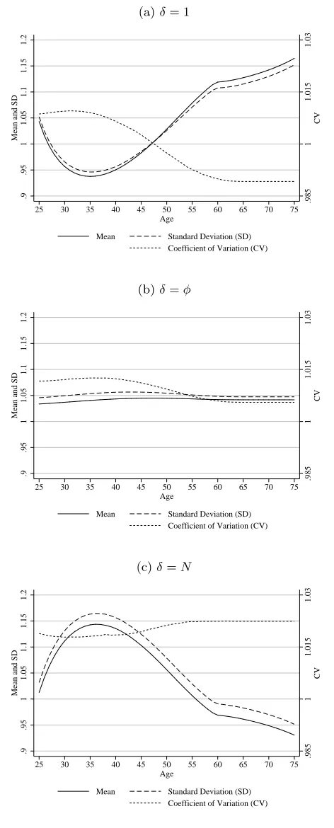
Figure 13 shows the CV for the Demographics model, under different utility weights, along
consumption means and standard deviations, all relative to theSinglemodel.
We already explained at length the pattern for equivalized consumption means and standard
deviations over the life-cycle for the different utility weights. Forδt6=φt, the CV follows a reversed
profile. Whenever consumption (and inequality) are low relative to the Single model (over the
life-cycle), the CV is large and vice versa.
Forδt= 1, in theDemographicsmodel households want to shift consumption away from periods
with large household size and save a lot during these periods even if being hit with large income
shocks. Compared to the Single model, this implies a relatively larger equivalized consumption
inequality (measured by the CV) even conditional on the lower equivalized consumption mean and
14
Figure 13: Equivalized Consumption: Means and Inequality
(a)δ= 1
.985 1 1.015 1.03 CV .9 .95 1 1.05 1.1 1.15 1.2
Mean and SD
25 30 35 40 45 50 55 60 65 70 75
Age
Mean Standard Deviation (SD) Coefficient of Variation (CV)
(b)δ=φ
.985 1 1.015 1.03 CV .9 .95 1 1.05 1.1 1.15 1.2
Mean and SD
25 30 35 40 45 50 55 60 65 70 75
Age
Mean Standard Deviation (SD) Coefficient of Variation (CV)
(c)δ=N
.985 1 1.015 1.03 CV .9 .95 1 1.05 1.1 1.15 1.2
Mean and SD
25 30 35 40 45 50 55 60 65 70 75
Age
Mean Standard Deviation (SD) Coefficient of Variation (CV)
absolute inequality (measured by the SD). In contrast, later in life (around age 47-48) the larger
amount of accumulated assets allows to insure against income shocks better relative to theSingle
model.
The opposite is true for the profile of the CV in the case that δt =Nt. In the Demographics
model, households want to allocate consumption to periods where household size is large. During
these time periods, the CV is the lowest. Bad income shocks are smoothed by eating up savings
and by borrowing against future income. Later in life, this behavior results in a higher CV. Over
the entire life-cycle, relative equivalized consumption inequality as measured by the CV is higher
in theDemographics model than in theSinglemodel. Hence, the higher life-time resources do not
only lead to a larger absolute equivalized consumption inequality (as measured by the SD) but also
to a larger relative equivalized consumption inequality (as measured by the CV).
This latter effect is also present for the case of δ = φ, i.e. the CV is again higher in the
Demographics model in all periods. The equivalized consumption profile is steeper earlier in life in
theDemographics model because households accumulate more savings. This is because households
in theDemographics model share savings among its member if they eat them up to smooth income
shocks.15 However, given household size and equivalence scales, they are less willing to do so early
in the life-cycle. This explains the increase of the CV early in life and the decrease later in life as
higher savings can be used for insurance. This whole line of argumentation has of course to be seen
relative to theSinglemodel.
The main insight from this discussion, is that even in this scale-free measure, we detect
differ-ences between the predictions of the Singlemodel and the equivalizedDemographics model. After
controlling for differences in mean consumption, implied inequality in theDemographics models can
be up to 2% higher than from the Singlemodel. Furthermore, incentives for self-insurance change
over the life-cycle, not only because of the degree of uncertainty but also because of the interplay
between uncertainty and household size and composition which (depending on the utility weight
δ) provides additional motives for consumption-savings decisions.
15
Figure 14: Number of “Adult Equivalents” for Different Equivalence Scales
.5
1
1.5
2
2.5
3
3.5
OECD NAS HHS SR DOC LM Nelson
No Child One Child Two Children Three Children
Note: For explicit formulations of the different equivalence scales, see Table 1 inFern´andez-Villaverde and Krueger (2007).
7.3 Different Equivalence Scales
In Figure 14 we compare the implied value of equivalence scales, for different household sizes.
The vertical axis measures the number of “adult-equivalent” members in the household. Below, we
expand our analysis for the OECD and Nelson scales. These choices follow closely the discussion of
equivalence scales in Fern´andez-Villaverde and Krueger (2007) as the OECD scale has the lowest
economies of scale while the opposite is true for the Nelson scale. Furthermore, the square root
scale “SR” is almost identical to the “Mean” scale in Fern´andez-Villaverde and Krueger (2007)
which is their preferred choice.
In Figure 15we show equivalized consumption for the different utility weights and equivalence
scales considered. All the profiles are in terms of consumption from the single agent model. Recall
from Figure 14, the OECD scale has the lowest economies of scale; put differently, is the closest
in value to N. On the other hand, the Nelson scale has the highest economies of scale and is the
closest to 1. The square root scale falls between the two. From Figure 15, we see that the ratio
Figure 15: Equivalized Consumption Relative toSingleModel
(a)δ= 1
.8
.9
1
1.1
1.2
25 30 35 40 45 50 55 60 65 70 75
Age
Square Root OECD Nelson
(b)δ=φ
.8
.9
1
1.1
1.2
25 30 35 40 45 50 55 60 65 70 75
Age
Square Root OECD Nelson
(c)δ=N
.8
.9
1
1.1
1.2
25 30 35 40 45 50 55 60 65 70 75
Age
Square Root OECD Nelson
scales, determines the size of the difference between the Demographics and the Singlemodel over
the life-cycle: the bigger the difference between this ratio and one, the bigger the increase in the
bias over the life-cycle introduced by the equivalization of household data (as long as δ is not set
exactly toφ).
For example, when we consider the OECD equivalence scale and theδt=Ntas utility weight (a
case when the ratio is closest to one, Figure15c), differences in equivalized consumption across the
Demographics andSinglemodels are milder than when we consider theδt= 1 case (when the ratio
deviates the most from one, Figure 15a). The opposite is true for the Nelson scale: equivalized
consumption from the model with utility weights of δt = Nt are the ones that result in the most
extreme differences with the Single model. The intuition behind the shape of these figures is the
same that we discussed previously for the square root scale.
When the utility weight is exactly equal to the equivalence scale (δt = φt), the profiles of
equivalized household and single household consumption are very similar throughout. However,
the relative value of equivalized lifetime income is lower the higher the equivalence scale. Hence,
for the OECD scale, the relative difference between equivalized household and single household
consumption is greater than for the square root and Nelson scales.
As seen from Figure 15b, the best case scenario for theSinglemodel is when the utility weight
equals the equivalence scale (δt=φt), see Figure15b) and the equivalence scale is the one provided
by Nelson: in that case, the differences between the predictions of equivalized consumption across
models is the smallest (around 1% each period). This is due to the fact that the Nelson scale
admits the highest economies of scale among all considered equivalence scales, meaning that the
effect of household size on household income and consumption is very mild. In simple terms, given
that with the Nelson scaleφt≈1 for allt, andδt=φt, in this case both theDemographics and the
Singlemodels behave very similarly.
In terms of equivalized consumption inequality, the resulting figures are very similar to Figure
15 for the standard deviations and the logic behind is similar. Given incomplete markets and
idiosyncratic income shocks, periods in which households want to consume more, consumption is
more subject to reflect income shocks, and thus, consumption inequality is higher. We therefore
only present the CVs in Figure16. For the cases where δt 6=φt, we still find that the further the
Figure 16: Coefficient of Variation Relative to SingleModel
(a)δ= 1
.98
.99
1
1.01
1.02
1.03
25 30 35 40 45 50 55 60 65 70 75
Age
Square Root OECD Nelson
(b)δ=φ
.98
.99
1
1.01
1.02
1.03
25 30 35 40 45 50 55 60 65 70 75
Age
Square Root OECD Nelson
(c)δ=N
.98
.99
1
1.01
1.02
1.03
25 30 35 40 45 50 55 60 65 70 75
Age
versus the Singlemodel over the life-cycle. E.g. as argued before, for δt= 1, the large value of the
OECD scale compared to the Nelson scale makes the households in theDemographicsmodel much
less willing to consume when household size is large and thus, to consume out of savings. As a
consequence, the CV relative to theSingle model increases much more early in life for the OECD
scale compared to the Nelsons scale which is however reversed later in life. From here we conclude
that the single approach to modeling consumption, not only introduces absolute but also relative
differences in inequality. Moreover, these differences vary over the life-cycle.
8
Discussion: value of
δ
and
φ
We have discussed at length different cases for utility weights and equivalence scales and the
sources of differences between whatDemographicsandSinglemodels predict. However, the question
still remains with regard to which values we should consider for empirical work. For example,
Hong and R´ıos-Rull (2007) set the utility weights to one,16 while Fuchs-Sch¨undeln (2008) sets it
equal to the equivalence scale. In both papers no further justification for this choice is provided.
Given the utility function chosen by Attanasio et al.(1999) and their parameter estimates for
ζ1, ζ2 and α in equation (1) allows us to back outδ for a given equivalence scale φ, by comparing
the preferences in (1) and in (2):
exp(ξ1Nad+ξ2Nch) =
δ(Nad, Nch)
φ(Nad, Nch)1−α
∀ Nad, Nch. (42)
For Nad = 1 and Nch = 0, our setup implies δ = φ = 1 whereas the preference parameter in
Attanasio et al. (1999) is expζ1. We therefore normalize the utility function (1) from their setup
by dividing it with this factor such that
δ(Nad, Nch) = exp(ζ1[Nad−1] +ζ2Nch)φ(Nad, Nch)1−α (43)
Note that it is not possible to uniquely pin down individual household member weights but only
the sum of the weights given by δ. In Figure17, we show the calculated δt/φt ratios, for different
household sizes and various equivalence scales. In addition, we plot the the two extreme cases
16
we considered in the quantitative analysis, δt = 1 and δt = Nt, and a utility weight of δt = φt,
represented by a flat line equal to 1, as reference points.
For the OECD scale, probably the most common choice as equivalence scale (for example, see
Krueger et al. (2010)) the estimates byAttanasio et al.(1999) imply a ratioδt/φt close to one. In
terms of equivalized consumption means and inequality (relative to the single model) this case is
associated with the top profile in Figure15b and thus, the largest deviation from theSinglemodel
among the three considered scales. For the Nelson scale, the implied δt/φt ratio comes closest to
theδt=Ntcase which implies the largest deviation from the single model in terms of means (and
volatilities) depicted in Figure 15c by the profile that exhibits the most extreme differences with
respect to theSinglemodel.
Figure 17 shows that for the Square Root scale, theδt/φt ratio is right between the bands and
is higher than one. Since the ratio is clearly different from one (the case with the least amount of
bias introduced by the equivalization ofDemographics models) our results raise concerns about the
reliability of the single household framework.
Our main conclusion from this section is that, given the limited empirical evidence available,
predictions from the single household approach are likely biased, no matter the choice of equivalence
scale used.
9
Discussion and Future Work
We want to stress that our analysis, although being mostly quantitative, is still of theoretical
nature. E.g. deviating from the assumption that the discount factorβwas set to one and the interest
rate to zero, or more generally from β(1 +r) = 1, will interact with the life-cycle consumption
and savings decisions and might downplay or accelerate the differences between the two models.
The question remains as to how important would these biases be in a state of the art model of
consumption and income which we will consider for future work. Furthermore, we still need to
explore additional factors which might affect the consumption-savings problem of the household,
and thus, create differences to predictions of single agent models: zero borrowing constraints,