Catch limits, capacity utilization and cost reduction in Japanese fishery management

Munich Personal RePEc Archive

Catch limits, capacity utilization and

cost reduction in Japanese fishery

management

Yagi, Michiyuki and Managi, Shunsuke

Graduate School of Environmental Studies, Tohoku University,

Graduate School of Environmental Studies, Tohoku University

24 January 2011

Online at

https://mpra.ub.uni-muenchen.de/96385/

1

Catch limits, capacity utilization and cost reduction in Japanese fishery management

Michiyuki Yagi1 _{and Shunsuke Managi}1,2*

1 _{Graduate School of Environmental Studies, Tohoku University, 6-6-20 Aramaki-Aza Aoba,}

Aoba-Ku, Sendai 980-8579, Japan. Email: yagimichiyuki@gmail.com

2 _{Institute for Global Environmental Strategies, Japan. Email: managi.s@gmail.com (* Corresponding}

Author)

Abstract

Japan’s fishery harvest peaked in the late 1980s. To limit the race for fish, each fisherman could be

provided with specific catch limits in the form of individual transferable quotas (ITQs). The market

for ITQs would also help remove the most inefficient fishers. In this article we estimate the potential

cost reduction associated with catch limits, and find that about 300 billion yen or about 3 billion dollars

could be saved through the allocation and trading of individual-specific catch shares.

Keywords: Capacity output; Capacity utilization; Individual quotas; Production frontier; Japan

JEL codes: L70; Q18; Q22

Citation

Yagi, M., Managi, S., 2011. Catch limits, capacity utilization and cost reduction in Japanese fishery management. Agricultural Economics 42 (5), 577–592. doi:10.1111/j.1574-0862.2010.00533.x

[Submitted 21 February 2010; revised 26 June 2010; accepted 21 November 2010]

For the accepted version, please visit Agricultural Economics website below:

2 1. Introduction

Excess capacity in fisheries and over-exploitation of fish resources is associated with

reduced food production potential and economic waste (Food and Agriculture Organization, 2008a).

The race to expand harvesting of wild fish exemplifies the tragedy of the commons and has long been

a subject for research in resource economics (i.e., Gordon, 1954). Management of this common-pool

resource remains difficult, however, leading to a declining volume of fish caught for developed

countries from 1979 through 2005 (FAO, 2008b).

Fisheries in Japan, as in many other countries, are both biologically and economically

overexploited (Pascoe et al., 2004). Japanese fishery catches have been decreasing over the last two

decades. For example, catches in 2006 totaled about 55,000 metric tons (Fig. 1), which is only 44%

of 1987 production (FAO, 2008b). The number of vessels and fishermen has also been diminishing to

a 2006 level of 210,246 and 212,470 vessels and fishermen, respectively, down from 308,335 and

411,040 in 1987 (MAFF, 2007). The exit of fishermen has kept labor productivity (i.e., the quantity of

fish caught per worker) and capital productivity (i.e., value per fishing vessel) relatively stable for all

fish excluding sardines, with a maximum fluctuation of 20%.

Takarada and Managi (2010) describe a negative spiral of overexploitation in the Japanese

fishing industry, with a race for fish among fishermen who invest in new capacity to capture as much

of the remaining fish stocks as possible. As the fish stock decreased in the late 1980s, these individuals’

profits began to diminish. In response, an additional increase in the fishing effort occurred in an

attempt to recover previous economic losses. Then, the fish stocks kept decreasing due to further

fishing efforts, and the fishermen faced the need to increase their efforts or exit the industry. As a result,

the Japanese fishing industry has been shrinking for decades as a market. In fact, the number of the

coastal fishing boats and the production numbers for coastal fisheries are decreasing continuously

(MAFF, 2005a).

To stop the downward spiral associated with overuse of an open-access resource, fishery

policies in Japan include the total allowable catch (TAC) and total allowable effort (TAE) systems,

3

transfers (GFTs). The TAC is a catch limit set for a particular fishery, generally for a year or a fishing

season and is usually expressed in tonnages of live-weight equivalent but is sometimes set in terms of

numbers of fish (OECD, 1998). The TAE sets an upper limit on the number of fishing days and the

number of operating vessels in a specific area within the exclusive economic zone (EEZ).1

For the purpose of resource management, however, these fishery policies need to be further

examined. The fisheries in Japan remain open access resources because their TAC caps have been too

loose to restrict the activity of fishermen. In most cases, until 2009 in Japan, the TAC caps were higher

than the allowable biological catch (ABC) figures, which indicate the level of stock that accounts for

the scientific uncertainty in the estimate of overfishing limit. In addition, financial support seems to

merely maintain capacity at a stable level rather than attempting to control fishery capacity.

In this article, we analyze the profit potential in Japan’s fishery industry that would follow

from the allocation of optimal, individually specific catch limits. Keeping in mind the importance of

fishery management and production in Japan, this study analyzes the quantitative potential of optimal

input/output allocation by assigning optimal individual quotas (IQs). Our results show the ideal case

for the potential IQ system in one respect. The catch shares of the IQ system divide the total permitted

catch in a fishery into shares (Macinko and Bromley, 2002). That is, under these systems, yearly limits

or quotas are set for a fishery.2 This ensures that, given the scientifically allowable total catch, a

percentage share of that total can be allocated to fishermen based on the level of calculated optimal

output for each region/fisherman.

1 In consideration of the declining fish catches, the Japan Fisheries Agency enacted the “Basic Law on Fisheries Policy” in June 2001. The law presents new guidelines for fishery policy, replacing the “Coastal Fishery and Others Promotion Law” of 1963, whose primary aim was to improve fishery productivity. The Basic Law includes two key concepts: (1) securing a stable supply of fishery products and (2) the sound development of the fisheries industry to promote the appropriate conservation and management of marine life resources.

4

The more in-depth purpose of this study is to measure the fishing capacity of Japan’s

fisheries. Then, we examine how much cost reduction they can achieve in a well-controlled world

using unique disaggregated data covering all areas of Japan. We also aim to determine the optimal

inputs/outputs mix of Japanese fisheries given fishery quotas. It is also important to recognize how

much capacity will be necessary when the TAC system, which is apparently too loose at present,

tightens up as individual transferable quotas (ITQs). This offers criteria for stringent quota

enforcement. In addition, we consider technical inefficiencies due to differences in fishery areas and

fishing types under different conditions and variant distributions of fish stocks.

Previous research has often aimed to measure the degree of excess capacity among fishing

fleets, in terms of capacity output and capacity utilization (CU). Fishing capacity is the maximum

amount of fish over a period of time (a year or season) that can be produced by a fishing fleet if fully

utilized, given the biomass and age structure of the fish stock and the present state of the technology,

whereas capacity output represents the maximum level of production that the fixed inputs are capable

of supporting under normal working conditions (see FAO, 2003, 2008a; Färe et al., 1994; Johansen,

1968; Kirkley et al., 2003; Morrison, 1985). CU is the proportion of available capacity that is utilized

and is usually defined as the ratio of actual (i.e., current) output to some measure of capacity (i.e.,

potential) output (see Kirkley et al., 2003; FAO, 2003, 2008a; Morrison, 1985; Nelson, 1989).

Therefore, CU is measured on a 0 to 1 scale. When CU is less than 1, one could produce a better catch

than the current catch if inputs were fully utilized. In other words, smaller inputs are sufficient

(assuming they are fully utilized) to produce a catch of the current size.

In this study, we use the revised Johansen industry model to measure capacity outputs

following Kerstens et al. (2006). This model uses two steps involving different linear programming

(LP) techniques. First, we measure the capacity output by using output-oriented data envelopment

analysis (DEA). Then, we measure the optimal fixed inputs given in certain fishery quotas. Optimal

scales for outputs and fixed factor inputs indicate the required total outputs and inputs at the industry

level. The calculated loss of efficiency shows the possible reduction in the fixed inputs. The capacity

5

calculated based on the maximum outputs given current inputs.

The data used in this study come from the 11th Fishery Census of Japan of 2003 and the

Annual Statistics on Fishery and Fish Culture 2003 by the Ministry of Agriculture, Forestry and

Fisheries of Japan. The data sets include each aggregated fishery entity in each municipality and for

each marine fishery type in the whole of Japan, and they contain a wealth of data at the whole industrial

level. Note it is not clear how much of the fleet has changed since 2003. Furthermore, the census data

do not include individual data per vessel. Capacity output and CU in this study are estimated not per

vessel as defined in previous studies but instead per municipality per marine fishery type. Our

estimation method could be applied to other data, however, and is provided as a MATLAB program

together with the Japanese data alongside the online version of this article at the publisher’s website.

2. Background 2.1. Policies in Japan

In 1995, the Japan Fisheries Agency started to reduce the number of fishing vessels and

restrictions on fishing area and/or period for some fisheries to ensure the sustainable use of fishery

resources. The TAC system has also been implemented. The principal laws are “The Fisheries Law,”

the “Living Aquatic Resources Protection Law,” and the “Law Concerning the Conservation and

Management of Marine Living Resources.” These principal laws were also amended in keeping with

the concept of the “Basic Law on Fisheries Policy.” The central and prefectural governments regulate

fishing efforts in terms of fishing methods. The TAC system assigns TAC allocations to each fishery

separately but not to individual fishermen. While seven fish species are subject to the TAC system,

covering about 30% of total fishing in Japan in 2000, the TAE was established as a system for

managing total allowable effort with the amendment of the “Law Concerning Conservation and

Management of Marine Living Resources.” The TAE includes curtailing the number of boats, the

suspension of operations, and the improvement of fishing gear, among others. However, these

6

regulations are too loose to control the actual activities of fishermen.

Meanwhile, the amount of GFTs related to fisheries in Japan (JPY 271 billion in 2003),

which tends to decline slightly over the past 10 years, is much larger than in most OECD countries

(OECD, 2006). The largest portion of GFTs related to fisheries in Japan is allocated to the construction

of coastal infrastructure (JPY 203 billion in 2003), i.e., fishing ports and other coastal public facilities,

among others. The other forms of financial support provided by Japan to the fishing industry are direct

payments for fishery restructuring (JPY 2 billion in 2003), interest subsidies (JPY 3 billion in 2003),

which are designed to facilitate the structural adjustment of coastal fisheries under certain conditions,

and general services expenditures (JPY 62 billion in 2003; OECD, 2006). The amounts of GFTs

providing direct payments for restructuring and interest subsidies are much lower than those for the

others. These subsidies apparently are justified because they do not contribute to the increase in fishing

capacity.

2.2. Review of methodologies

There have been many studies that have focused on fishing capacity and measured capacity

output and CU for decades. The assessment methods for estimating CU can be roughly classified into

two groups: parametric methods and nonparametric methods. In one example of the use of parametric

methods, Kirkley and Squires (1988) introduce a hedonic cost function approach to estimating the

aggregate capital stock and investment in a fishery utilizing limited information. They use vessel

acquisition price and vessel characteristics in New England from 1965 to 1981. Although these data

have several limitations, the results indicate that the investment in New England fisheries appears to

have increased over time. The largest increase in investment occurred in 1979, after the passage of the

Magnuson Fisheries Conservation and Management Act of 1976.

Similarly, Asche et al. (2008) adopt a parametric approach that includes cost and profit

functions, with survey data for costs and earnings. They investigate potential rents and overcapacity

in five case studies in Norway, Sweden, Denmark and the U.K. (countries that use individual vessel

7

Based on their cost and earnings data, the actual level of economic profits earned by these fisheries,

with the exception of Iceland, was found to be negligible. However, the results show that more than

half of the vessels were potentially redundant, and potential economic profits were estimated to be

between 22% and 61% of revenue in all case studies.

In another case using parametric approaches, Felthoven and Morrison Paul (2004) develop

a multi-output and multi-input stochastic function framework considering changing output

compositions at full capacity to estimate capacity output and CU. They use the model to analyze

catcher-processor vessels in the Alaskan pollock fishery. The average capacity utilization measure in

2001 ranges from 0.65 for a scenario with the flatfish catch held constant to 1.1 for a scenario assuming

unrestricted output composition. The former implies that the pollock catch could increase by about

53% on average with the same level of flatfish landings. The latter suggests that economic optimization

over outputs will result in less pollock being caught. The authors also find that for many vessels, there

is a divergence between the output price ratio of pollock to flatfish and the marginal rate of

transformation (i.e., output trade-offs).

In addition, there are also many studies using nonparametric approaches, usually the DEA

approach, to estimate capacity output and CU. Tingley and Pascoe (2005a) estimated the CU of four

U.K. fleet segments using the DEA model following Färe et al. (1989, 1994) and examined some

factors affecting CU via tobit regression analysis. The results indicate that the average CU of otter

trawling vessels, beam trawling vessels, scallop dredging vessels, and gill netting vessels in U.K.

fisheries are 0.88, 0.67, 0.78, and 0.70, respectively, and show that they could increase their outputs

by 14%, 50%+, 28%, and 43%. The results of the tobit analysis suggest that changes in stock

abundance are the main factor affecting CU, although the overall statistical quality of the models was

poor.

Based on Färe et al. (2001), Kerstens et al. (2006) have developed a sophisticated variation

on the multi-output/input frontier-based short-run Johansen industry model. In the industry model, the

capacity of individual fishery entities is utilized by minimizing fixed industry inputs given their total

8

are allowed to vary and be fully utilized. The authors use the industry model to analyze the capacity

outputs of the Danish fleets, analyzing scenarios including tightening quotas, seasonal closure policies,

lower and upper bounds, decommissioning schemes, and area closures. The results show that vessel

numbers can be reduced by about 14% and the use of fixed inputs by around 15%, depending on the

specific objective and the policy mix at a specific Danish fishery. Tingley and Pascoe (2005b) uses an

industry adjustment model which is in line with Kerstens et al (2006) to find the effects of introducing

ITQs on fleet structure and profitability.

3. Model

3.1. Industry model

Following the revised short-run Johansen model by Kerstens et al. (2006), we compute

marine fishery efficiencies in Japan. The conceptual model proceeds via two steps. In the first step,

the capacity measures are compared to determine capacity production for each fishery entity at the

production frontier. Capacity production is calculated using the output-oriented DEA model assuming

strong disposal of inputs and outputs and VRS (see Managi et al. (2004) for intuitive explanation of

the DEA). In the second step, individual entity capacities are utilized and fixed industry inputs are

minimized given total outputs, capacities, and the current state of the technology. This capacity

measure is short-run because it does not assume any change in existing firm-level capacity and because

it is a technical rather than an economic capacity notion. Another reason is that it also assumes constant

stocks.

The following models are used in this study. The production technology S transforms inputs

𝑥 = (𝑥1, . . . , 𝑥𝑛) ∈ 𝑅+𝑛 _{into outputs 𝑢 = (𝑢1, . . . , 𝑢𝑚) ∈ 𝑅+}𝑚 _{and summarizes the set of all feasible}

input and output vectors: 𝑆 = {(𝑥, 𝑢) ∈ 𝑅+𝑛+𝑚_{: 𝑥 𝑐𝑎𝑛 𝑝𝑟𝑜𝑑𝑢𝑐𝑒 𝑢}. Let J be the number of regional}

units. The n-dimensional input vector x is partitioned into fixed factors (indexed by f ) and variable

factors (indexed by v): 𝑥 = (𝑥𝑓, 𝑥𝑣) . To determine the capacity output and CU, a radial

9

given the current input use: 𝐸0_{(𝑥, 𝑦) = 𝑚𝑎𝑥{ 𝜃: (𝑥, 𝜃𝑦) ∈ 𝑆}.}

Boat capacity output is defined as the maximum amount that can be produced per unit of

time with existing equipment (assuming that the availability of variable factors of production is not

restricted). The term “boat” capacity is used where the term “plant” capacity is used for other industry

applications. In the context of fisheries, this definition corresponds to the maximum catch that a vessel

can produce if the present technology is fully utilized given the biomass and the age structure of the

fish stock under general working conditions. We note that this definition does not measure the capacity

output level that can only be realized at a prohibitively high cost of input usage (and that hence will

be economically unrealistic). This is because this boat capacity measure does not allow the reallocation

of inputs and outputs across firms and implicitly assumes that the production of capacity output is

feasible and that the necessary variable inputs are available (Kerstens et al., 2006). The production

technology 𝑆̂ of boat capacity can be represented as follows:

𝑆̂𝑉𝑅𝑆_{= {(𝑥, 𝑢) ∈ 𝑅}

+𝑁+𝑀: 𝑢𝑗𝑚≤ ∑ 𝑧𝑗𝑢𝑗𝑚, 𝐽

𝑗=1

𝑚 = 1, . . . , 𝑀; ∑ 𝑧𝑗𝑥𝑗𝑓≤ 𝐽

𝑗=1

𝑥𝑗𝑓,

𝑓 = 1, . . . , 𝐹; ∑ 𝑧𝑗= 1 𝐽

𝑗=1

, 𝑧𝑗≥ 0, 𝑗 = 1, . . . , 𝐽}

(1)

The output-oriented efficiency measure θ1 is measured using the following LP problem for

each decision-making unit (DMU) (region or firm) j (j = 1, 2, ..., J) relative to the set of short-run

production possibilities. Here we use most disaggregated regional unit as DMU as j:

𝑚𝑎𝑥 𝜃₁𝑗,𝑧𝑗

{𝜃₁𝑗: (𝑥, 𝜃₁𝑗𝑢) ∈ 𝑆̂𝑉𝑅𝑆_}

(2)

To be consistent with the boat capacity definition, only the fixed inputs are bounded at their

observed level, and the variable inputs in the production model are allowed to vary and be fully utilized.

The computed outcome of the model is a scalar θ1. The θ1 shows by how much the production of each

output in each region can be increased. In particular, capacity output for region k of the mth output is

𝜃1∗𝑘 multiplied by actual production, ukm. Therefore, capacity utilization based on observed output

10

CU 𝑜𝑜𝑘 =_𝜃1

1∗𝑘 (3)

This ray CU measure may be biased downward (see Färe et al., 1994). This is because there

is no guarantee that the observed outputs are not produced in a technically efficient way. The problem

of technically efficient measures is solved when both the variable and the fixed inputs are constrained

to their current level. Another technical efficiency measure is obtained by evaluating each region j =

1, 2, ... , J relative to the production probability set SVRS_:

𝑆𝑉𝑅𝑆_{= {(𝑥, 𝑢) ∈ 𝑅+}𝑁+𝑀_{: 𝑢}

𝑗𝑚≤ ∑ 𝑧𝑗𝑢𝑗𝑚, 𝐽

𝑗=1

𝑚 = 1, . . . , 𝑀; ∑ 𝑧𝑗𝑥𝑗𝑛≤ 𝐽

𝑗=1

𝑥𝑗𝑛,

𝑛 = 1, . . . , 𝑁; ∑ 𝑧𝑗 = 1 𝐽

𝑗=1

, 𝑧𝑗 ≥ 0, 𝑗 = 1, . . . , 𝐽}

(4)

The outcome (θ2) shows by how much production can be increased using technically

efficient inputs:

𝑚𝑎𝑥 𝜃₂𝑗,𝑧𝑗

{𝜃₂𝑗: (𝑥, 𝜃₁𝑗𝑢) ∈ 𝑆𝑉𝑅𝑆_{} (5)}

The technically efficient output vector is θ2 multiplied by the amount of observed production

for each output. The unbiased ray measure of capacity utilization (subscripted “eo”) is calculated as

follows:

CU𝑒𝑜 𝑘 =𝜃2 ∗𝑘

𝜃₁∗𝑘 (6)

The unbiased measure of capacity is not the technically efficient output. The first measure

includes both technical efficiency and capacity utilization effects; while the second measure includes

only the technical efficiency effects, thus by dividing them provides the capacity utilization (i.e., it is

unbiased) (see Färe et al., 1989; Felthoven and Morrison Paul, 2004; Holland and Lee, 2002).

We focus on reallocating catches between vessels by explicitly allowing improvements in

technical efficiency and capacity utilization rates. The model is developed in two steps as follows. An

optimal activity vector z∗k _{is provided for region k from model (1), and thus, capacity output and the}

11 𝑢𝑘𝑚∗ = ∑ 𝑧𝑗∗𝑘𝑢𝑗𝑚− 𝑠𝑗𝑚∗𝑘;

𝑗

𝑥𝑘𝑓∗ = ∑ 𝑧𝑗∗𝑘𝑥𝑗𝑓+ 𝑠𝑗𝑓∗𝑘; 𝑗

𝑥𝑘𝑣∗ = ∑ 𝑧𝑗∗𝑘𝑥𝑗𝑣

𝑗 (7)

where 𝑠𝑗𝑚∗𝑘 and 𝑠𝑗𝑓∗𝑘 are the optimal surplus and slack variables corresponding to the output

and fixed input dimensions, respectively. In a second step, these “optimal” frontier figures (i.e.,

capacity output and capacity variable and fixed inputs) at the regional level are used as parameters in

the industry model. In particular, the industry model minimizes the industry use of fixed inputs radially

such that the total production is at least at the current total level (or at a quota level in the model

extended later) based on the reallocation of production between regions. Reallocation is allowed based

on the frontier production and input usage for each region. In the short term, we assume that current

capacities cannot be exceeded at either the regional or the industry level. We define Um as the industry

output level of output m and Xf (Xv) as the aggregate fixed (variable) inputs available to the sector of

factor f(v); i.e.,

𝑈𝑚= ∑ 𝑢𝑗𝑚; 𝑗

𝑋𝑓= ∑ 𝑥𝑓𝑗; 𝑗

𝑋𝑣= ∑ 𝑥𝑣𝑗

𝑗 (8)

The formulation of the multi-output and frontier-based industry model can then be specified

as follows:

𝑚𝑖𝑛 𝜃,𝑤,𝑋𝑣𝜃

s.t. ∑ 𝑢𝑗𝑚∗ 𝑤𝑗 ≥ 𝑈𝑚, 𝑚 = 1, . . . , 𝑀, 𝑗

     ∑ 𝑥𝑓𝑗∗ 𝑤𝑗≤ 𝜃𝑋𝑓, 𝑓 = 1, . . . , 𝐹, 𝑗

     −𝑋𝑣+ ∑ 𝑥𝑣𝑗∗ 𝑤𝑗≤ 0, 𝑗

𝑣 = 1, . . . , 𝑉,

     0 ≤ 𝑤𝑗 ≤ 1, 𝜃 ≥ 0, 𝑗 = 1, . . . , 𝐽,

(9)

where the optimal activity vector w represents a weight assigned to the vessel’s peers to estimate its

capacity output.

12

We now turn to the second-stage industry model (9). First, based on the second modification

above, the constraints for each output dimension must reflect the fact that production may take place

in different areas. That is, there are M output constraints (species) for each of the A areas:

∑ 𝑢𝑗𝑚𝑎∗ 𝑤𝑗𝑎∗ ≥ 𝑈𝑚𝑎, 𝑗

𝑚 = 1, . . . , 𝑀, 𝑎 = 1, . . . , 𝐴 ₍₁₀₎

Here, the data in this study are municipality data for each fishery type. Therefore, the optimal

activity vector w∗ _{in this study denotes a weight allocated to each municipality to estimate each the}

capacity both in each fishery and each municipality.

Each region j has one area a that corresponds to the location of each aggregated entity. The

industry consists of fishery entities or vessels fishing in different areas. The constraints for each of the

total fixed inputs can be formulated in the most general way in terms of constraints indexed by area:

∑ 𝑥𝑓𝑗𝑎∗ 𝑤𝑗𝑎∗ ≤ 𝜃𝑋𝑓, 𝑗,𝑎

𝑓 = 1, . . . , 𝐹. ₍₁₁₎

The constraints on the variable inputs are as follows:

−𝑋𝑣+ ∑ 𝑥𝑣𝑗𝑎∗ 𝑤𝑗𝑎∗ ≤ 0, 𝑗,𝑎

𝑣 = 1, . . . , 𝑉. ₍₁₂₎

To offer a menu of current and potential conservation and distributional policies in fisheries,

we add some further refinements to the short-run industry model of Dervaux et al. (2000). Here, we

focus on four issues: (i) tightening quotas for each species and (ii) the partial tolerance of technical

inefficiencies. (i) We consider setting quotas such as the ITQs for particular species in Japan to

illustrate how much capacity is necessary given a certain quota. We simply add the constraint:

∑ 𝑈𝑚𝑎= 𝑈𝑚∙ 𝑎

𝑄𝑚,  𝑚 = 1,   0 ≤ 𝑄𝑚≤ 1 (13)

given that the species are indexed by m, which is equal to 1 (i.e., the first output). Qm indicates a quota

rate for the mth current industry output. In this study, Qm is incremented by 0.01 from 0 to 1 for the

purpose of a sensitivity analysis.

(ii) The frontier nature of the underlying technologies may push things too far so that it is

13

While technical efficiency is a condition for any social optimum, realistic planning procedures may

require tolerating technical inefficiency at some points for informational and political reasons (Peters,

1985).

This can be modeled by adjusting the capacity output, which is part of the second-stage

industry model, based on its current observed technical inefficiency and ultimately using an efficiency

improvement imperative (α) to correct it (see Kerstens el al., 2006). Of course, technically efficient

regions need no such adjustment at present. Therefore, assuming that this correction factor is smaller

than or equal to unity (α = 1), the adjustment of the second-stage capacity output could take the

following form when technical inefficiency is (partially) accepted:

𝜃 ≥ 0, 𝑢̂𝑗𝑚𝑎∗ = 𝑢𝑗𝑚𝑎 ∗

𝑚𝑎𝑥{ 1, 𝛼𝜃₁∗_}

𝑗 = 1, . . . , 𝐽, 𝑎 = 1, . . . , 𝐴

(14)

In this research, α is 0.1 or 0.2 for all the entities when technical inefficiency is partially

tolerated. When α is set as 0.1 or 0.2, the capacity outputs of all the entities are limited to 10 or 5 times

the current output.

We sum up the above-mentioned constraints, and our model can be presented as follows:

𝑚𝑖𝑛 𝜃,𝑤,𝑋𝑣𝜃

s.t. ∑ 𝑢̂𝑗𝑚𝑎∗ 𝑤𝑗𝑎∗ ≥ 𝑈𝑚𝑎, 𝑚 = 1, . . . , 𝑀, 𝑎 = 1, . . . , 𝐴 𝑗

     ∑ 𝑥𝑓𝑗∗ 𝑤𝑗𝑎∗ ≤ 𝜃𝑋𝑓, 𝑓 = 1, . . . , 𝐹 𝑗,𝑎

     −𝑋𝑣+ ∑ 𝑥𝑣𝑗∗ 𝑤𝑗𝑎∗ ≤ 0, 𝑣 = 1, . . . , 𝑉 𝑗,𝑎

     ∑ 𝑈𝑚𝑎= 𝑈𝑚⋅  𝑎

𝑄𝑚, 𝑚 = 1

      𝜃 ≥ 0, 𝑢̂𝑗𝑚𝑎∗ = 𝑢𝑗𝑚𝑎 ∗

𝑚𝑎𝑥{ 1, 𝛼𝜃1∗}

     𝑗 = 1, . . . , 𝐽, 𝑎 = 1, . . . , 𝐴,  0 ≤ 𝑤𝑗𝑎∗ ≤ 1,0 ≤ 𝑄𝑚≤ 1.

14 4. Data and scenarios

4.1. Data

The data used in this study come from the 11th Fishery Census of Japan of 2003 and Annual

Statistics on Fishery and Fish Culture 2003 by the Ministry of Agriculture, Forestry and Fisheries of

Japan. The data set is composed of each aggregated fishery entity per municipality per marine fishery

type in Japan. The 2003 Fishery Census of Japan was conducted to clarify the structures of fishery

production in Japan and to explore the overall background on fisheries, including fishing villages, the

marketing and processing industries, and other considerations. The purpose is to develop basic data

for fishery policies, including improvements to the structure of fisheries.

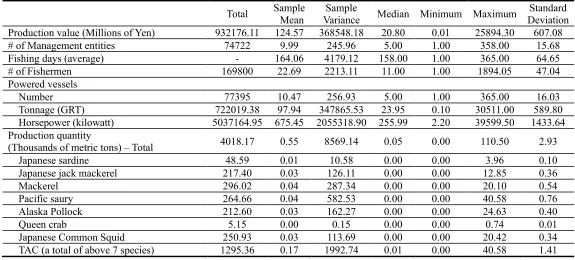
Our output data consist of production value data (in Japanese yen) and quantity data. There

are nine types of outputs used in this study: total production quantity, all fish, other marine animals,

Japanese sardines, Japanese jack mackerel, mackerel, Pacific saury, Alaska pollock, queen crab, and

Japanese common squid. The TAC system in Japan applies to all seven of these species. For example,

the squid showed a slight decline, although it still remains in a dominant position. The pollock has

been on the decline mainly due to the subsequent decrease in the catch on the Bering high seas.

Mackerel have also decreased drastically over the years.

There are two variable inputs, labor, and fishing days, and two fixed inputs of gross

registered, tons (Grt), and horse power (kilowatt), for aggregated fishery entities in each municipality

and for each marine fishery type in Japan. The variable inputs are the number of workers on board at

peak times and average fishing days for each aggregated entity. These data effectively cover all of the

Japanese fishery entities. In total, 74,728 fishery entities are covered as part of the data set of 7,483

observations. The total product value of these data accounts for 89.3% of the original data in the census.

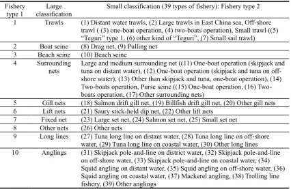
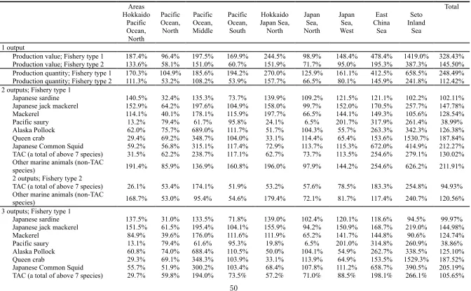
On average, each aggregated fishery entity consists of about 10 entities. We have 39 marine fishery

classifications (Table 1). Small whaling, diving fisheries, shellfish collecting, seafood collecting, and

other fisheries are excluded because we consider these fisheries to be atypical cases.

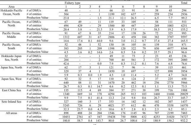
We assume that management decisions are provided on the disaggregated regional level,

15

particular fishery type. Thus, the efficiency of each aggregated fishery entity is evaluated relative to

one of the potentially 351 different technologies (nine areas multiplied by thirty-nine marine fishery

types). The technologies, which consist of only a few similar observations, may lead to biases in the

estimation of boat capacity due to a lack of comparable production units. To avoid downward

estimation, we use 10 large classifications and refer to the 10 and 39 fishery classifications as fishery

types 1 and 2, respectively (see Table 1). Therefore, there are potentially 90 different technologies

being used in fishery type 1 and 351 in type 2. We mainly use fishery type 1 and compare type 1 with

type 2 in an unconstrained scenario.

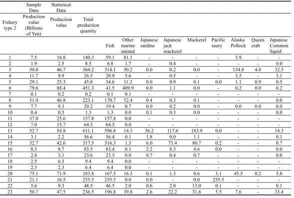
4.2. Scenarios

In each specification, we use several different types of output variables. In the first two

specifications, production value and production quantity are used as the output variables, and we

compare the two levels of efficiency. Then, we divide the estimated production quantity into three

categories, which are (a) TAC species, and the others including (b) fish and (c) the other marine

animals. The aim of this division is to set production quotas only for particular TAC species and to

compare the efficiency levels of the different groups.

We classify a series of scenarios, systematically testing the effect of additional constraints.

The results of several policy-oriented scenarios with various constraints are useful in indicating policy

implications. These scenarios are summarized in Table 2. Basic scenario 1 is the basic industry model

without any particular constraints and uses fishery type 1. Basic scenario 2 uses fishery type 2 without

any particular constraints. The tolerated technical inefficiency scenario allows for technical

inefficiency but already imposes improvement imperatives of 1,000% and 500% (thus, α = 0.1 and

0.2). We compute the optimal inputs in the industry model, implementing the 100% quota for current

outputs (which is, essentially, no quota constraint (i.e., Q1 = 1 in Eq. (13)) at each technical inefficiency

value.

We also estimate optimal fishery expenditures at the current 100% quota to understand how

16

particular: expenditure on vessels, fishing gears, oil, and wages, which appear to change as the amount

of fishery inputs varies. However, we have only the production value data as mentioned above.

Therefore, we roughly estimate the fishery expenditures related to marine fishery operations using the

production value and the optimal inputs at current 100% quota levels.

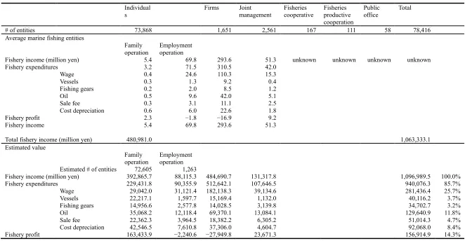
We use the number of marine fishery entities and the average fishery income and

expenditures by organization type as well as total fishery income for fishery households and the whole

of the industry according to the 11th Fishery Census of Japan of 2003 and Statistical Survey Report

on Fishery Management of 2003 (Table 3). We consider only four kinds of organizations: individuals,

including family businesses and independent fishermen; firms; and joint management. These are the

categories used to calculate the fishery income and expenditures in the whole industry, while the others

are not included because we have no detailed earnings statements for them and the numbers of entities

in these fishery organizations is low. We compute the numbers of family businesses and employment

operations based on the total fishery income for fishery households, and we estimate the fishery

income and expenditures for the whole fishing industry in Japan. Although there is indeed only a small

difference between the actual value and the estimated value for total fishery income, the total estimate

values for vessels, fishing gear, oil, wages, and cost depreciation are 3.7%, 3.2%, 11.8%, 25.7%, and

8.4% of the total estimated fishery income, respectively.

First, to estimate cost reduction in the scenarios analyzed, we simply multiply the total

fishery income of the sample data, 932.2 billion yen, by the fishery expenditure ratios estimated above

and the total estimated expenditures on vessels, fishing gear, oil, wages, and cost depreciation in the

sample, which amount to 34.1, 29.5, 110.2, 239.2, and 78.2 billion yen, respectively. Then, we assume

that the expenditures on vessels and fishing gear are correlated with the efficiency score, i.e., θ in Eq.

(15).We also assume that the oil costs are correlated with the optimal use of tonnage multiplied by the

number of fishing days at the current 100% quota; i.e., ∑(𝑤𝑗∗⋅ 𝑥𝑓,1∗ ) ⋅ (𝑤𝑗∗⋅ 𝑥𝑣,1∗ ). Finally, we assume

that the wage costs relate to the optimal use of labor multiplied by the number of fishing days at the

current 100% quota, i.e., ∑(𝑤𝑗∗⋅ 𝑥𝑣,1∗ ) ⋅ (𝑤𝑗∗⋅ 𝑥𝑣,2∗ ) . To estimate the expenditures, we multiply the

17

fishing gear), oil, and wages in the first step by θ, ∑ 𝑤𝑗∗2⋅𝑥𝑓,1∗ ⋅𝑥𝑣,1∗

(𝑋𝑓,1⋅𝑋𝑣,1) and

∑ 𝑤𝑗∗2⋅𝑥𝑣,1∗ ⋅𝑥𝑣,2∗

(𝑋𝑣,1⋅𝑋𝑣,2) , respectively.

5. Empirical results 5.1. Scenario analysis

5.1.1. Current and capacity outputs

Scenarios 1 and 2 show the results achieved by comparing current output and capacity

outputs (see Fig. 2). In the figure, the vertical and horizontal axes represent percentages of total

production values and fixed inputs, respectively. The results are calculated with LP and show what

production values fixed inputs can maximally produce based on each scenario. Similarly, Fig. 3 shows

what production quantities the fixed inputs can maximally produce based on each scenario.

The results indicate that there is large excess capacity in Japanese fisheries. This reflects the

fact that fisheries management is in a state of crisis. Because access is almost free, fishing activity is

under-priced, and therefore, a huge amount of effort is devoted to fishing. Based on the concept of

constant returns to scale, 1% of the total fixed inputs produces 1% of the total outputs, and the path of

the current output will be linear. Note that efficiency implies the average efficiency of each scenario

if we do not specify otherwise. This is because current output is calculated with LP, which seeks to

combine DMUs to minimize a requisite amount of the fixed inputs for a certain amount of output. On

the other hand, the more varied the efficiency levels of the aggregated entities are, the more curved

the line of capacity outputs becomes because 1% of the total outputs can be produced by less than 1%

of the fixed inputs.

Comparing the current outputs of the production values and quantities in Fig. 3, the current

output of the production values has a less curved line than that of the quantities. This implies that each

DMU determines the amount of fixed inputs depending on expected values rather than expected

quantities and that this is legitimate decision making depending on the estimation of income and

expenditures for each fishery.

18

of the production values are smaller than those of the quantities. The difference between these numeric

values may result from the varied efficiency levels based on the entities’ valid decision-making and

cost-benefit considerations.

5.1.2. Capacity outputs

We show two results indicating efficiency levels using the production value data and the

quantity data. First, Fig. 4 shows the capacity outputs of production values based on each scenario.

Sensitivity analyses are provided by changing the total quota, and in each case, efficiency is computed.

The quota is used as the horizontal line in the figure. Here, inefficiency in this figure is defined as a

percentage reduction of fixed inputs and is determined by applying Eq. (15). According to the results,

efficiency levels based on 100% of production value (i.e., the current level of production) as the total

quota are 0.102 in basic scenario 1 and 0.169 in basic scenario 2. In the scenarios at current 100%

quotas considering areas of technical inefficiency of up to 10 and 5 times, efficiency scores of 0.156

(0.239) and 0.210 (0.292) emerge in the scenarios using fishery type 1 (type 2), and the efficiency

scores decrease by approximately 5% at regular intervals as α varies from 1 to 0.1. Fig. 5 shows the

capacity output of computed product quantities based on each scenario. The results show efficiency

levels at the 100% quota of 0.072 and 0.130 in basic scenarios 1 and 2, respectively. These scenarios

are relatively efficient and similar to those for production value. In the scenarios at the current 100%

quotas considering technical inefficiency of up to 10 and 5 times, the efficiency scores 0.96 (0.170)

and 0.125 (0.197) emerge in the scenarios using fishery type 1 (type 2), and the efficiency scores

decrease by about 2.5% at regular intervals as α drops from 1 to 0.1.

5.1.3. TAC species

We show the results of the sensitive analyses achieved by only imposing a quota on the TAC

species as ITQ. Figure 6 shows the result achieved when the total product quantities are separated into

two groups: the quantity for all TAC species and that for all non-TAC species. The efficiency scores

19

each scenario curve alongside each other and are approximately parallel. In the scenarios at current

100% quotas considering technical inefficiency of up to 10 and 5 times, the efficiency scores 0.135

(0.205) and 0.168 (0.231) emerge in the scenarios using fishery type 1 (type 2), respectively, and the

efficiency scores decline by about 3% at regular intervals as α varies from 1 to 0.1.

Additionally, Fig. 7 shows the results that are achieved when the total product quantities are

divided into three categories: the quantities for TAC species, those of other fish, and those for other

marine animals. The paths of each scenario are also approximately parallel alongside each other.

Efficiency levels at the 100% quota are 0.145 and 0.190 in basic scenarios 1 and 2, respectively. In the

scenarios at the current 100% quotas considering technical inefficiency of up to 10 and 5 times, the

efficiency scores 0.177 (0.222) and 0.204 (0.246) emerge in the scenarios using fishery type 1 (type

2), respectively.

We also provide the results that are achieved when we impose a quota on each of the six

TAC species. First, Fig. 8 shows the results using two categories: (1) the six TAC species and (2) one

other species. Given a 100% ITQ quota, the efficiency levels in the scenarios for Japanese sardines,

Japanese jack mackerel, and mackerel are 0.086, 0.088, and 0.089, respectively, and the efficiency

paths for these species vary slightly as each ITQ quota decreases. At a 100% ITQ quota, efficiency

levels in the scenarios for Pacific saury, Alaska pollock, and Japanese common squid are 0.093, 0.099,

and 0.099, respectively. The efficiency paths vary more than those for the others as each ITQ quota

decreases. The efficiency level of the queen crab fishery is 0.084 at a 100% ITQ quota, and the

efficiency path is the lowest found in any of the scenarios.

In contrast, the efficiency of basic scenario 1, which imposes a quota on total quantities of

all TAC species, is 0.109 if the current industry quota is used. The score is the most inefficient found

in any of the scenarios. This result suggests that there are fewer activity vectors to choose from for the

aggregated entities to satisfy the quota for each TAC species. In this case, the quota is imposed only

on a certain TAC species, and thus, the other fisheries have the capacity to catch 100% of current

output. Therefore, there are fewer options in choosing fixed input factors given that quota imposed on

20

Fig. 9 shows the results using each of six TAC species, other fish and other marine animals.

Efficiency levels at a 100% quota are 0.109 in the Japanese sardine scenario, 0.110 in the Japanese

jack mackerel scenario, 0.112 in the Mackerel scenario, 0.118 in the Pacific saury scenario, 0.117 in

the Alaska pollock scenario, 0.108 in the queen crab scenario, 0.139 in the Japanese common squid

scenario and 0.145 in the all-TAC-species scenario. The efficiency paths of the Japanese sardine and

queen crab scenarios are the lowest, and that of the all-TAC-species scenario is the most inefficient.

The same is true for the paths using two variables above. Most scenarios for each TAC species are

stationary at less than 60% of each quota.

These varied efficiency levels depend on the selection of outputs. When each output in each

category is separated in different model, the efficiency score will become even lower. It is difficult to

measure the efficiency of each fishery method because there are many fishery species in the Japanese

sea and many fishery methods developed in the same regions. While we can estimate efficiency levels

in various detailed cases using more disaggregated categories, it will become difficult to discuss entire

fisheries in Japan in doing so. The opposite is also true. Based on the results, the efficiency paths seem

to be approximately the same in the different cases; they only vary based on the quota for each TAC

species.

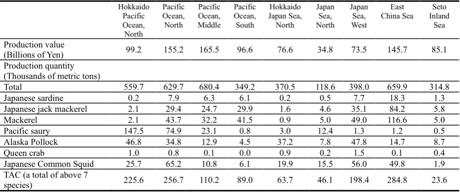
In summary, ensuring the current capacity outputs (except for certain TAC species), the fixed

inputs can satisfy the capacity outputs for the TAC species. Regarding the capacity output of the total

quantity per fishery area in basic scenarios 1 and 2, the most efficient area is the Pacific Ocean in the

north. Most areas have excess capacity of more than 100% in basic scenario 2. This result implies that

there are fixed inputs that can produce more than twice the current quantities in Japan.

The fisheries with the lowest excess capacity are those for Pacific saury. There are excess

capacities of 39.0% and 38.9% for Pacific saury using two variables and three variables as above

(fishery type 1). The most inefficient fisheries are those for Japanese common squid, with excess

21 5.1.4. Capacity utilization

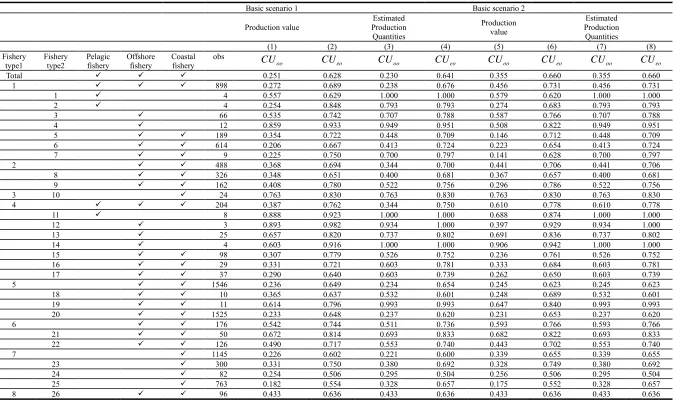
We estimate the CUoo and CUeo of total production value and quantity in basic scenarios 1

and 2. Table 4 presents simple average CUoo and CUeo figures for the aggregated entities. These are

not weighted average values, and they are classified by fishery types 1 and 2. There are significant

differences between the values of CUoo and CUeo for the different fishery types.

In the basic scenario 1 using estimated quantity data (specifications 3 and 4), the fisheries

with the highest average CUoo, i.e., CUoo = 1, are large trawls in East China sea, large and medium

surrounding net of one-boat operation catching skipjack and tuna on distant water and two-boats

operation with purse seine (fishery type 2: (2), (11) and (14)). In specification 3, the fishery with the

lowest average CUoo is anglings (fishery type 1: (10)), and the CUoo is 0.113.

In specification 4, the fisheries with the highest average CUeo (i.e., CUeo = 1) are large trawls

in the East China Sea, large and medium catching skipjack and tuna in distant waters and off-shore

water, two-boat operations with purse seine, and squid angling in distant water (fishery type 2: (2),

(11), (12), (14) and (34)). In specification 4, the fishery with the lowest average CUeo is squid angling

in coastal water (fishery type 2: (36)); the CUeo is 0.486.

The difference between CUeo and CUoo shows the degree of random variation in catch and

technical inefficiency, which is not producing the full potential given the level of both fixed and

variable inputs. The fisheries with the lowest differences between CUeo and CUoo (i.e., CUeo – CUoo =

0) are distant water trawls, large trawls in the East China Sea, large and medium catching skipjack and

tuna in distant water, two-boat operations with purse seine and billfish drift gill nets (fishery type 2:

(1), (2), (11), (14) and (19)). The fishery with the greatest difference between the CUeo and CUoo

figures is angling (fishery type 1: (10)), and the difference value is 0.459.

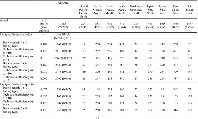
5.2. Reducing the number of fishery entities

We compute the amount of non-zero activity vectors w∗ _{from the results above and provide}

the optimal number of aggregated fishery entities at the current 100% quota for each sea area around

22

optimal total number of fishery entities at a 100% quota are as follows: (1) 1,167 at a minimum in the

technically tolerated inefficiency scenario up to 10 times of each current output using one variable

output and (2) 2,692 at a maximum in the technically tolerated inefficiency scenario up to 10 times of

each current output using the three variable outputs.

On average the optimal total DMU numbers are about 2,000. The values of the activity

vectors are almost at upper limits among all the scenarios (i.e., all inputs are utilized).We compute the

numbers of fishery entities, which is 74,727 in the overall sample, by multiplying the active vector

values and the numbers of entities in each aggregated entity level. The minimum number is 4,974.7 in

the basic scenario 1 using the quantities data of one variable output. The maximum number is 21,184.7

in the basic scenario 2 using the production value data allowing technical inefficiency up to five times

of each current output.

We note that there are large differences among the optimal sizes of fishery entities in each

scenario at 100% quota. On average, however, the optimal size of the current Japanese fisheries fishing

the amount of current production value/quantity is about one third of current size. In other words, one

third of the current fishery entities are required even if the central government implements fishery

policies in the most efficient way.

5.3. The optimal input levels

We compute the optimal input amounts at the current 100% quota for each scenario. In each

scenario at the current 100% quota, the optimal input values in gross registered tons and horsepower

(kilowatts) are equal to each efficiency score, i.e., θ. In each similar scenario, we set the average

optimal fishing days as the simple average 𝑤𝑗∗⋅ 𝑥𝑣,1∗ among DMUs with 𝑤𝑗∗≠ 0 and the optimal

number of fishermen as ∑ 𝑤𝑗∗⋅ 𝑥𝑣,2∗ .

Under basic scenarios 1 and 2, using the production value data at the 100% quota, the

average optimal numbers of fishing days are 113.32% and 112.72% of the current average fishing days

spent on board, and the total optimal numbers of fishermen are 35.69% and 43.81% of the current

23

10 and 5 times current outputs using the production quantity data for fishery type 1 (type 2), the

average optimal numbers of fishing days are 119.43% (114.81%) and 120.45% (116.50%) of the

current average fishing days spent on board, and the total optimal numbers of fishermen are 41.62%

(53.83%) and 48.59% (58.45%) the current totals, respectively. In summary, in each scenario at the

100% quota, the optimal numbers of fishermen and the optimal average fishing days are about 40%

and 120% of current totals.

Going through the amounts of optimal inputs for each fishery type, we see that the most

efficient way of allocating the fishery types is different for specific fishery types. In addition, a fishery

type with a large amount of optimal inputs may not be an efficient method itself but may yield large

capacity outputs arising from optimal inputs based on the first step, the revised industry model.

Relatively large amounts of optimal inputs are needed in types of surrounding nets (4), lift nets (6) and

fixed nets (7) among others, and long lines (9) in particular are little utilized.

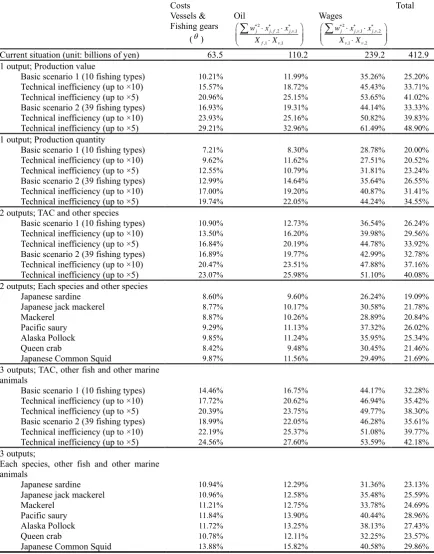
5.4. Estimates of cost reduction

We compute the fishery expenditures for each scenario in Table 5. Overall, the required costs

of vessels, fishing gear, and oil (in our computed cases) are mostly less than about 20% of current

costs, and the wages and total costs are mostly about 40% and 30%, respectively. In basic scenario 1

(basic scenario 2), using one output variable for the production value, the necessary costs of vessels

and fishing gear, oil, and wages amount to 10.21% (16.93%), 11.99% (19.31%), and 35.26% (44.14%),

and the overall costs amount to 25.20% (33.33%), respectively.

The reduction in the total number of fishing vessels represents a large amount of the

reduction in the total cost in the long run. These significant potential results are important for policy

purposes. In basic scenario 1 (scenario 2), using the production value data, the results imply that the

current estimated fishery profit (total 133.3 billion yen) will be increased to 442.2 (408.6) billion yen.

In addition, the fishery profits should increase because the cost depreciation related to the fishery

24 6. Discussion and conclusion

This article examines the capacity output and CU of marine fisheries in Japan. Our results

indicate that the maximum level of production that the fixed inputs are capable of supporting under

general working conditions (i.e., capacity output) could be more than three times larger than what is

currently produced. Estimated CUs vary greatly from one marine fishery to another, but overall fixed

inputs could be reduced to one tenth of their current level. Fishery profits could be increased to about

three times their current level.

Our results for Japan indicate much greater potential for improvement than Kerstens et al.

(2006) found for Denmark. The differences between the two scenarios are caused by the large

differences in fishery management level (or efficiency). The creation of profitable and sustainable

fisheries requires retiring the most inefficient fishers, through a government-backed industry

development program. This study does not discuss the details of input and output control policies.

Political factors often favor input-oriented approaches to managing fisheries. However, there appears

to be increasing acceptance of output-oriented controls used to manage catches of target fishes

(Holland, 2007). Our approach is not market-based but we show the expected outcome of

output-oriented controls. For the output-output-oriented controls to be implemented inexpensively, improvements in

remote automated monitoring technology need to increase the feasibility and then diminish the cost of

outcome controls.

Our study shows that there are many inefficient fisheries. To help them exit the industry,

buyback programs may need to be increased. However, higher government subsidies should be

carefully considered before they are implemented. Simple buyback programs that purchase inefficient

vessels out of a fishery will not help to solve the overcapacity problem (see Asche et al., 2008; Clark

et al., 2005; Holland et al., 1999). First, the buyback programs might at best remove only a marginal

portion of the fishing fleets, with less efficient vessels remaining in the fisheries. Secondly, buyback

programs will not work properly without other work opportunities for fishermen who leave a fishery.

Additionally, incentives remain for vessels to increase their own level of capitalization. Finally, even

25

fisheries and local communities because there is a close relationship between the number of vessels

and the number of fishermen. This development would run counter to social policies concerned with

protecting societies along remote coastlines (Asche et al., 2008).

In conclusion, legislating for property rights over fisheries is necessary to stop the

downward spiral of this industry. Our approach estimates the optimal cost reduction and profitability

that is achievable under Japan’s current fishing activity management system, run by central planners.

One might also consider potential efficiency in fisheries based on other mechanisms such as individual

transferrable quotas (ITQs) (MAFF, 2008). Either way, the potential magnitude of gains demonstrated

in this article has important implications for fisheries policy in Japan and elsewhere.

Acknowledgments

We acknowledge Research Institute of Economy, Trade and Industry (RIETI) and Ministry

of Environment, and Grant-in-Aid for Scientific Research from the Japanese Ministry of Education,

Culture, Sports, Science and Technology (MEXT) for the financial support. We would like to thank

Yukichika Kawata, William A. Masters, and two anonymous referees and participants at IIFET 2008

and RIETI seminar for useful comments. All remaining errors are our own.

Supporting Information

Data Appendix Available Online: A data appendix to replicate main results is available in the online

version of this article.

26 References

Asche, F., Eggert, H, Gudmundsson, E., Hoff, A., Pascoe, S., 2008. “Fisher’s behavior with individual vessel quotas−over-capacity and potential rent Five case studies.” Marine Policy 32, pp.920–927.

Clark, C.W., Munro, G.R., Sumaila, U.R., 2005. “Subsidies, buyback, and sustainable fisheries.” Journal of Environmental Economics and Management 50, pp.47–58.

Costello, C., Gaines, S.D., Lynham, J., 2008. “Can catch shares prevent fisheries collapse?” Science 321, pp.1678–1681.

Dervaux, B., Kerstens, K., Leleu, H., 2000. “Remedying excess capacities in French surgery units by industry reallocations: the scope for short and long term improvements in plant capacity utilization.” In J. Blank (ed.)., 2000. “Public Provision and Performance: Contribution from Efficiency and Productivity Measurement.” Amsterdam: Elsevier, pp.121–146.

Färe, R., Grosskopf, S., Kerstens, K., Kirkley, J., Squires, D., 2001. “Assessing shortrun and medium-run fishing capacity at the industry level and its reallocation.” In Johnston, R. S. Shriver, A. L., (eds), “Microbehavior and Macroresults: Proceedings of the Tenth Biennial Conference of the International Institute of Fisheries Economics and Trade.” pp.10–14, July 2000, Corvallis, Oregon, USA, Corvallis: International Institute of Fisheries Economics and Trade.

Färe, R., Grosskopf, S., Kokkelenberg, E.C., 1989. “Measuring Plant Capacity, Utilization and Technical Change: A Nonparametric Approach.” International Economic Review 30, pp.655–666.

Färe, R., Grosskopf, S., Lovell, C.A.K., 1994. “Production Frontiers.” Cambridge: Cambridge University Press.

FAO of the United Nations, 2008a. “Fisheries Management: 3. Managing fishing capacity.” FAO Technical Guidelines for Responsible Fisheries 4(3), FAO/21916/G, (Rome, FAO, 2008a). FAO of the United Nations, FishStat Plus, Fisheries and Aquaculture Information and Statistics

Service, Global Aquaculture Production, 1950–2005 (Rome: FAO, 2008b), http://www.fao.org/fishery/topic/16073 (accessed on 8 April 2008).

FAO of the United Nations, 2003. “Measuring capacity in fisheries.” In Pascoe, S., Gréboval, D., (eds), FAO Fisheries Technical Paper 445.

Felthoven, R. G., Morrison Paul, C. J., 2004. “Multi-Output, Nonfrontier Primal Measures of Capacity and Capacity Utilization.” American Journal of Agricultural Economics 86(3), pp.619–633. Gordon, H.S., 1954. “The economic theory of a common property resource: the fishery.” Journal of

political economy 62, pp.124–142.

Holland, D.S, Gudmundsson, E., Gates, J., 1999. “Do fishing vessel buyback programs work: A survey of the evidence.”Marine Policy 23(1), pp.47–69.

Holland, D.S., 2007, “Managing environmental impacts of fishing: input controls versus outcome-oriented approaches,” International Journal of Global Environmental Issues 72(3), pp.255– 272.

Holland, D.S., Lee, S.T., 2002. “Impacts of random noise and specification on estimates of capacity derived from data envelopment analysis.” European Journal of Operational Research 137, pp.10–21.

Johansen, L., 1968. “Production functions and the concept of capacity.” Namur, Recherches Re´centes sur la Fonction de Production, Collection ‘Economie Mathe´matique et Econometrie’, n8. Kerstens, K., Vestergaard, N. and Squires, D., 2006. “A Short-Run Johansen Industry Model for

Common-Pool Resources: Planning a Fisheries' Industry Capacity to Curb Overfishing.” European Review of Agricultural Economics 33(3), pp.361–389.

Kirkley, J.E., Squires, D., Alam, M.F., Ishak, H.O., 2003. “Excess capacity and asymmetric information in developing country fisheries: The Malaysian purse seine fishery.” American Journal of Agricultural Economics 85(3), pp.647–662

Kirkley, J.E., Squires, D.E., 1988. “A limited information approach for determining capital stock and investment in a fishery.” Fishery Bulletin 86(2), pp.339–349.

27 Resource Economics.” Island Press.

Managi, S., Opaluch, J.J., Jin, D. and Grigalunas, T.A. 2004. “Technological change and depletion in offshore oil and gas.” Journal of Environmental Economics and Management 47(2): 388– 409.

Ministry of Agriculture, Forestry and Fisheries of Japan (MAFF), 2008. “Japan’s Concept of Individual Transferable Quotas.” Ministry of Agriculture, Forestry and Fisheries of Japan, Tokyo. < http://www.jfa.maff.go.jp/suisin/yuusiki/dai5kai/siryo_18.pdf >

Morrison, C., 1985. “Primal and dual capacity utilization: An application to productivity measurement in the U.S. automobile industry.” Journal of Business and Economic Statistics 3, pp. 312– 324.

Nelson, R., 1989. “On the measurement of capacity utilization.” Journal of Industrial Economics 37, pp.273–286.

Organisation for Economic Co-operation and Development (OECD), 2006. “Financial Support to Fisheries: Implications for Sustainable Development.” OECD Publishing.

Pascoe, S., Gréboval, D., Kirkley, J., Lindebo, E., 2004. “Measuring and Appraising Capacity in Fisheries: Framework, Analytical Tools and Data Aggregation.” FAO Fisheries Circular No.994, FIPP/C994(En).

Peters, W., 1985. “Can inefficient public production promote welfare?” Journal of Economics 45, pp.395–407.

Statistics Department – Ministry of Agriculture, Forestry and Fisheries (MAFF), 2007. “Annual Statistics of Fishery and Fish Culture 2006.”

Statistics Department – Ministry of Agriculture, Forestry and Fisheries (MAFF), 2005a. “The 11th (2003) Fisheries Census.”

Statistics Department – Ministry of Agriculture, Forestry and Fisheries (MAFF), 2005b. “Annual Statistics of Fishery and Fish Culture 2003.”

Statistics Department – Ministry of Agriculture, Forestry and Fisheries (MAFF), 2005c. “Statistical Survey Report on Fishery Management of 2003.”

Takarada, Y., Managi, S., 2010. “Resource Economics: Case Study for Fishery.” Minervashobo Publisher, Tokyo.

Tingley, D., and Pascoe, S., 2005a. “Factors Affecting Capacity Utilisation in English Channel Fisheries. ” Journal of Agricultural Economics 56 (2), pp.287–305.

28

1980 1990 2000

0 2000 4000 6000 8000 10000 12000 14000

Th

o

u

sand

met

ri

c

to

n

s

Year

inland waters fishery aquaculture

coastal fishery offshore fishery pelagic fishery

Fig.1 Trend of Fishery Catch in Japan

29

0%

20%

40%

60%

80%

100%

0%

20%

40%

60%

80%

100%

Fixed Input

P

roduc

ti

on va

lue

Current situation

Capacity output (Basic scenario 1)

Capacity output (Basic scenario 2)

30

0% 20% 40% 60% 80% 100%

0% 20% 40% 60% 80% 100%

Fixed Input

P

roduc

ti

on qua

nti

ty

Current situation

Capacity output (Basic scenario 1) Capacity output (Basic scenario 2)

31

100% 80% 60% 40% 20% 0%

0% 5% 10% 15% 20% 25% 30% 35%

Basic scenario 1 Basic scenario 2

Tech inefficiency (up to 10 times) (type 1) Tech inefficiency (up to 10 times) (type 2) Tech inefficiency (up to 5 times) (type 1) Tech inefficiency (up to 5 times) (type 2)

Ef

fic

ie

nc

y

Value of fishery production

32

100% 80% 60% 40% 20% 0%

0% 5% 10% 15% 20% 25%

Basic scenario 1 Basic scenario 2

Tech inefficiency (up to 10 times) (type1) Tech inefficiency (up to 10 times) (type2) Tech inefficiency (up to 5 times) (type1) Tech inefficiency (up to 5 times) (type2)

Ef

fic

ie

nc

y

Quota

33

100% 80% 60% 40% 20% 0%

0% 5% 10% 15% 20% 25%

Basic scenario 1 Basic scenario 2

up to 10 times (type1) up to 10 times (type 2) up to 5 times (type1) up to 5 times (type 2)

Ef

fic

ie

nc

y

Quota

34

100% 80% 60% 40% 20% 0%

0% 5% 10% 15% 20% 25%

Basic scenario 1 Basic scenario 2

Tech inefficiency (up to 10 times) (type 1) Tech inefficiency (up to 10 times) (type 2) Tech inefficiency (up to 5 times) (type 1) Tech inefficiency (up to 5 times) (type 2)

Ef

fic

ie

nc

y

Quota

35

100%

80%

60%

40%

20%

0%

0.000

0.025

0.050

0.075

0.100

0.125

TAC

Japanese sardine

Japanese jack mackerel

Mackerel

Pacific saury

Alaska pollock

Queen crab

Japanese common squid

Ef

fic

ie

nc

y

Quota

36

100% 80% 60% 40% 20% 0%

0.000 0.025 0.050 0.075 0.100 0.125 0.150

TAC

Japanese sardine Japanese jack mackerel Pacific saury

Alaska pollock Queen crab

Japanese common squid squid

Ef

fic

ie

nc

y

Quota

37

Table 1. Technology (marine fisheries)

Fishery

type 1 classificationLarge Small classification (39 types of fishery): Fishery type 2 1 Trawls (1) Distant water trawls, (2) Large trawls in East China sea, Off-shore

trawl ( (3) one-boat operation, (4) two-boats operation), Small trawl ((5) “Teguri” type 1, (6) other kind of “Teguri”, (7) Small sail trawl)

2 Boat seine (8) Drag net, (9) Pulling net 3 Beach seine (10) Beach seine

4 Surrounding

nets Large and medium surrounding net ((11) One-boat operation (skipjack and tuna on distant water), (12) One-boat operation (skipjack and tuna on off-shore water), (13) Other than skipjack and tuna, one-boat operation), (14) boats operation, Purse seine ((15) One-boat operation, (16) Two-boats operation, (17) Other surrounding nets)

5 Gill nets (18) Salmon drift gill net, (19) Billfish drift gill net, (20) Other gill nets 6 Lift nets (21) Saury stick-held dip net, (22) Other lift nets

7 Fixed net (23) Large set net, (24) Salmon set net, (25) Small set net 8 Other nets (26) Other nets

9 Long lines (27) Tuna long line on distant water, (28) Tuna long line on off-shore water, (29) Tuna long line on coastal water, (30) Other long lines

10 Anglings (31) Skipjack pole-and-line on district water, (32) Skipjack pole-and-line on off-shore water, (33) Skipjack pole-and-line on coastal water, (34) Squid angling on distant water, (35) Squid angling on off-shore water, (36) Squid angling on coastal water, (37) Mackerel angling, (38) Trolling line fishery, (39) Other anglings

Table 2. Scenario Options

Scenario Constraints of formulation (17) involved Basic Scenario 1 =0; 0Q₁1; fishery type 1

Basic Scenario 2 =0; 0Q₁1; fishery type 2 Tolerating technical

inefficiency (up to ×10) =0.1; 0Q11; fishery type1 or 2

Tolerating technical