Imitating the Most Successful Neighbor in Social Networks

Munich Personal RePEc Archive

Imitating the Most Successful Neighbor

in Social Networks

Tsakas, Nikolas

Universidad Carlos III de Madrid

23 March 2012

Online at

https://mpra.ub.uni-muenchen.de/45210/

Imitating the Most Successful Neighbor in Social Networks

∗

Nikolas Tsakas

Department of Economics, Universidad Carlos III de Madrid

February 25, 2013

Abstract

We consider a model of observational learning in social networks. At every period, all agents

choose from the same set of actions with uncertain payoffs and observe the actions chosen by

their neighbors, as well as the payoffs they received. They update their choice myopically,

by imitating the choice of their most successful neighbor. We show that in finite networks,

regardless of the structure, the population converges to a monomorphic steady state, i.e. one

at which every agent chooses the same action. Moreover, in arbitrarily large networks with

bounded neighborhoods, an action is diffused to the whole population if it is the only one

chosen initially by a non–negligible share of the population. If there exist more than one

such actions, we provide an additional sufficient condition in the payoff structure, which ensures

convergence to a monomorphic steady state for all networks. Furthermore, we show that without

the assumption of bounded neighborhoods, (i) an action can survive even if it is initially chosen

by a single agent, and (ii) a network can be in steady state without this being monomorphic.

Keywords: Social Networks, Learning, Diffusion, Imitation.

JEL Classification: D03, D83, D85.

∗_{I am indebted to Antonio Cabrales for his support and suggestions which have significantly improved this paper.}

I would like to thank as well Friederike Mengel, Pedro Sant’anna, Daniel Garcia, Ignacio Ortu˜no, Elias Tsakas and seminar participants at Maastricht University, Universidad Carlos III de Madrid and the 4th World Congress of Game Theory Society GAMES 2012, for useful comments. Obviously, all remaining errors are my sole responsibility.

†_{E-mail: ntsakas@eco.uc3m.es; Universidad Carlos III de Madrid, Department of Economics, Calle Madrid 126,}

1.

Introduction

1.1.

Motivation

A common characteristic of most economic activities is that they are not organized on a centralized

and anonymous way (Jackson, 2008). They rather involve bilateral interactions between agents,

which also tend to be local in nature. These interactions lead to the formation of social networks,

since they affect indirectly not only the direct neighbors of the agents, but also all neighbors of

their neighbors, etc. Sometimes, the network may represent how information is transmitted in the

population, rather than imposing direct payoff externalities.

Information transmission is a very important aspect, mainly in situations where agents base their

decisions on others’ experience. Several models analyze the ways in which agents are affected by

the information they receive. Recently, there is strong empirical evidence supporting the fact that

people tend to imitate successful past behavior (Apesteguia et al., 2007; Conley and Udry, 2010;

Bigoni and Fort, 2013). This literature provides evidence that in several dynamic decision problems,

the agents seem to behave as if they observe the actions of their neighbors, and they tend to imitate

those who did better in the past. There are several reasons that can justify this behavior. On the

one hand, agents may not be aware of the mechanisms controlling the outcome of their choices, hence

they need to experiment themselves or rely on past experience of those they can observe. On the

other hand, in certain environments, Bayesian updating may require calculations which are beyond

the computational capabilities of the agents, leading them to adopt simple “rules of thumb” (Ellison

and Fudenberg, 1993).

In this paper, we study imitation of successful past behavior in a society with a network structure.

In our environment, the network describes the transition of information and not direct interaction,

meaning that the decision of one agent does not affect the payoffs of the others. In particular, we

study a problem of dynamic decision making under uncertainty, where the agents observe the actions

and the realized payoffs of their neighbors. Subsequently, they update their decisions by imitating

that neighbor who received the highest payoff in the previous period – which is the so-called

“imitate-the-best” updating rule (Al´os-Ferrer and Weidenholzer, 2008).

An example that is very relevant to our setting is the parents’ decision about which school to send

their children to; or their decision about whether to send them to a public school or a private one (also

mentioned by Ellison and Fudenberg, 1993). It is apparent that the satisfaction of the parents by

such a decision is based mainly on the characteristics of the school itself, rather than on the decisions

the same school. It is also commonly observed that the parents make this decision relying mostly

on other parents’ previous experience. This happens mainly because of the difficulty lying on the

identification of the real quality of each school. Furthermore, information received by those who had

been extremely satisfied in the past tends to be more influential; an observation that leads directly

to our naive updating mechanism. One can also apply this setting to decision problems regarding

the adoption of alternative technologies by agents who are not informed about their profitability, or

the purchasing of a service, such as the choice of mobile telephone operator.

1.2.

Results

Formally, we consider a countable population forming an arbitrary network. In each period, every

agent chooses an action from a finite set of alternatives and receives a payoff, which is drawn from a

continuous distribution associated with the chosen action. The agents are not aware of the underlying

distributions and the payoffs do not depend on the choices of other agents. The draws are independent

for every agent, meaning that it is possible that two agents choose the same action and receive different

payoffs.1 _{After making their own decision, they observe the actions and realized payoffs of all their}

neighbors. Subsequently, they update their choice, imitating myopically the choice of that neighbor

who received the highest payoff in the previous round.

We show that, when the population is finite the network eventually converges with probability

one to a monomorphic steady state, meaning that all the agents will eventually choose the same

action. However, this action need not be the most efficient. This happens because each action is

vulnerable to sequential negative shocks that can lead to its disappearance. Our result is robust to

cases where only a fraction of the population revises its action each period, as well as to cases where

some agents are experimenting, choosing randomly one of the actions they observed.

The results differ significantly when we let the population become arbitrarily large. First of all,

without further restrictions we cannot ensure convergence to a monomorphic steady state. In fact,

convergence depends on whether or not the agents have bounded neighborhoods, i.e. on whether

there are agents who interact with a non-negligible share of the population.

Assuming bounded neighborhoods, we can ensure the diffusion of a single action, if this is the

only one chosen initially by a non-negligible share of the population. If this is not the case, then

we provide a counter example, where a network never converges to a steady state. Nevertheless, we

1

provide a sufficient condition in the payoff structure, which ensures convergence regardless of the

network structure. This condition is more demanding than first order stochastic dominance, thus

implying that in very large networks the diffusion of a single action is very hard to occur and it

demands a very large proportion of initial adopters, or a special network structure, or an action to

be much more efficient compared to all others. The fact that our sufficient condition disregards the

importance of the network architecture completely, makes it useful mostly for networks with small

upper bound in the size of the neighborhoods. The behavior of specific network structures would be

a very interesting topic for further research.

Once we drop the assumption of bounded neighborhoods, the properties of the network change

significantly. In this case, an action may survive, even if it is chosen initially by only one agent. This

happens because this one agent may affect the choice of an important portion of the population;

an observation that stresses the role of centrality in social networks. For instance, providing a

technology or a product to a massively observed agent, can affect seriously the behavior of the

population. Finally, we construct another example where a network is in steady state without this

being monomorphic, which contrasts what our result for finite population has established.

Concluding, our extensive study of “imitate-the-best” learning mechanism introduces questions,

which intend to act as a trigger for future research. The fact that learning is a natural procedure

in societies and that imitation of successful behavior is commonly observable in many aspects of

social life, makes the study of the topic important, promising and, at the same time, interesting and

fascinating.

1.3.

Related Literature

Our work is in line with the literature on observational learning. Banerjee (1992), Ellison and

Fudenberg (1995) and Banerjee and Fudenberg (2004) introduce simple decision models where agents

tend to rely on behavior observed by others, rather than experimenting themselves. Closer to our

work is Ellison and Fudenberg (1993), where agents choose between two technologies, and periodically

evaluate their choices. They introduce the concept of an exogenous “window width”, which plays a

role similar to the network structure in our case. The fact that their updating mechanism involves

averaging the performance of several agents makes it significantly different from our

”imitate-the-best” rule.

This paper is also related to the literature on learning from neighbors. Large part of this literaure

strategies.2 _{On the one hand, Bala and Goyal (1998) study social learning with local interactions,}

under myopic best-reply. Learning occurs through Bayesian update, using information only about

their own neighbors. They provide sufficient conditions for the convergence of beliefs: Neighborhoods

need to be bounded in order to ensure convergence to the efficient action, which is an issue that arises

also in our problem.3 _{Existence of a set of agents which is connected with everybod (often called the}

“royal family”) can be harmful for the society. This happens because, such a set may enforce the

diffusion of their action/opinion, even if it not the optimal for the society. On the other hand, Gale

and Kariv (2003) study a Bayesian learning procedure, but using a network and payoff structure

quite similar to ours. They show that, given the fact that agents information is non-decreasing in

time, the equilibrium payoff must be also non-decreasing and since they assume it to be bounded, it

must converge. Moreover, in equilibrium identical agents gain the same in expectation. In general, in

Bayesian procedures the agents accumulate information through time, which it is not the case in our

setting. Hence, it is normal that convergence will be harder to occur, but eventually not impossible.

Learning by imitation has also been studied extensively in the literature. Various models of

evolutionary game theory (see Weibull, 1995; Fudenberg and Levine, 1998) are using different types

of imitation processes. In particular, Vega-Redondo (1997) provides strong theoretical support to the

imitation of successful behavior. He studies the evolution of a Cournot economy, where the agents

adjust their behavior by imitating the agent who was the most successful in the previous period.

He concludes that, this updating rule leads the firm towards Walrasian equilibrium. Furthermore,

Schlag (1998) studies different imitation rules, in an environment with agents with limited memory

randomly matched with others from the same population. He concludes that the most efficient

mechanism is the one where an agent imitates probabilistically the other’s behavior if it yielded

higher payoff in the past, with probability being proportional to the difference between the realized

outcomes. In Schlag (1999), he extends his framework to infinite populations, where each agent is

randomly matched with two agents each time. Even though the settings in those papers are different,

they provide additional evidence about the validity of our mechanism.

The literature on imitation in networks focuses mainly on coordination games and prisoner’s

dilemma games (e.g., Eshel et al., 1998; Al´os-Ferrer and Weidenholzer, 2008; Fosco and Mengel,

2010). In these models, uncertainty comes from the lack of information about the choices made by

each agent’s neighbor. However, for each action profile, the payoffs are deterministic, which is not the

case in our environment. Closer to our work is the paper by Al´os-Ferrer and Weidenholzer (2008),

2

Where the agents maximize short-term utility based on observed behavior of their neighbors in the previous period.

3

By bounded neighborhood we mean that there existsK >0 such that the number of neighbors of every agenti

where the aim is to identify the conditions for contagion of efficient actions in the long-run, problem

similar to the one we study.

Our analysis focuses on the diffusion of behavior, as well as the long-run properties of a network.

Large part of the literature in diffusion restricts attention to best-response dynamics, and relates

the utility of adopting a certain behavior with the number, or proportion, of neighbors who have

adopted it already. Morris (2000) shows that maximal contagion occurs for sufficiently uniform

local interactions and low neighbor growth. Along the same line, Lopez-Pintado (2008) and Jackson

and Yariv (2007) look into the role of connectivity in diffusion, finding that stochastically dominant

degree distributions to favor diffusion.

The rest of the paper is organized as follows. In Section 2, we explain the model. In Section 3, we

provide the main results for networks with finite population. While, in Section 4 we study networks

with arbitrarily large population. Finally, in Section 5 we conclude and provide possible extensions.

2.

The Model

2.1.

The agents

There is a countable set of agents N, with cardinalityn and typical elementsi and j, mentioned as

population of the network.4 _{Each agent i ∈N takes an actiona}t

i from a finite set A ={α1, ..., αM},

at every period t= 1,2, ....Each a∈A yields a random payoff.

Uncertainty is represented by a probability space (Ω,F,P_{), where Ω is a compact metric space,}

F is the Borel σ-algebra, and P _{is a Borel probability measure. The states of nature are drawn}

independently in each period and for each agent. Hence, it is possible that two agents choose the

same action at the same period and they receive different payoffs.

There is a common stage payoff function U :A×Ω→R_{, with U(a, ω) being bounded for every}

actionaand continuous in Ω. We restrict our attention to cases where ∀a, a′ _{∈A,U(a,Ω) is a closed}

interval in R _{and U(a,Ω) =U(a}′_{,Ω), while at the same time}P _{has full support.}5

2.2.

The Network

A social network is represented by a family of sets N :={Ni ⊆N | i = 1, . . . , n}, with Ni denoting

the set of agents observed by agent i. Throughout the paper Ni is called i’s neighborhood, and is

4

In Section 3 we assume thatnis finite, whereas in Section 4 we assumento be arbitrarily large.

5

assumed to containi. The setsN induce a graph with nodesN, and edgesE =Sn

i=1{(i, j) :j ∈Ni}.

We focus on undirected graphs: as usual, we say that a network is undirected whenever for alli, j ∈N

it is the case thatj ∈Ni if and only ifi∈Nj. In the present setting, the network structure describes

the information transmission in the population. Namely, each agent i ∈N observes the action and

the realized payoff of every j ∈Ni.

A path in a network between nodes i and j is a sequence i1, ..., iK such that i1 = i, iK = j

and ik+1 ∈ Nik for k = 1, ..., K −1. The distance, lij, between two nodes in the network is the

length of the shortest path between them. The diameter of the network, denoted as dN, is the

largest distance between any two nodes in the network. We say that two nodes are connected if

there is a path between them. The network is connected if every pair of nodes is connected. We

focus on connected networks, however the analysis would be identical for connected components of

disconnected networks.6

2.3.

Behavior

In the initial period,t= 1, each agent is assigned, exogenously, to choose one of the available actions.7

After each period, t = 2,3, . . . the agents have the opportunity to revise their choices. We suppose

that they can observe the choices and the realized payoffs of their neighbors in the previous period.

According to these observations, they revise their choice by imitating the action of their neighbor

who earned the highest payoff in the previous period. Ties are broken randomly.8 _{Formally, for}

t >1,

at+1

i ∈

a∈A : a=at

k where k = argmaxj∈NiU(a

t j, ω

t

j) (1)

where ωt

j is the actual state of nature at t, for agent j. Throughout the paper, we refer to this

updating rule as “imitate-the-best” (see also Al´os-Ferrer and Weidenholzer, 2008).

Notice that, the connections among the agents determine only the information flow and do not

impose direct effects in each other’s payoffs. An important aspect of this myopic behavior is that

the agents discard most of the available information. They ignore whatever happened before the

previous round and even from this round they take into account only the piece of information related

to the most successful agent. This naive behavior makes the network vulnerable to extreme shocks,

which may be very misleading for the society.

6

A component is a non-empty sub-networkN′ _{such thatN}′ _⊂N,N′_{is connected and ifi∈N}′ _{and (i, j)∈Ethen}

j∈N′ _{and (i, j)∈E}′_. 7

We assume that every action inAis chosen initially by some agent .

8

2.4.

Steady state and efficiency

State of period t is called the vector which contains the action chosen by each agent at this period,

i.e. St _{= (a}t

i, . . . , atn). We denote by At = {αk ∈ A : ∃i ∈ N such that ati = αk} the subset of

the action space, A, which contains those actions that are chosen by at least one agent in period

t. Notice, that an action which disappears from the population at a given period, never reappears,

hence At⊆At−1 ⊆ · · · ⊆A1 ⊆A. In a given period t, its state is called monomorphic if every agent

chooses the same action, i.e. if there exists k ∈ {1, ..., M}, such thatat

i =αk for alli∈N. Also, the

population is in steady state if no agent changes her action from this period on, i.e. if St′

= St _for

all t′ _{> t. Throughout the paper, the idea of convergence refers to convergence with probability one.}

Finally, we call an action efficientif it is the one that yields the highest expected payoff. An action

is mentioned as more efficientthan another one if it yields higher expected payoff.

3.

Networks with finite population

In this section, we restrict our attention to networks with finite population. We prove that finite

networks always converge to a monomorphic steady state, regardless of the initial conditions and the

network structure. Moreover, any action can be the one to survive in the long-run.

Before presenting our main results, it is worth mentioning a remark regarding the complete

network. In a complete network, each agent is able to observe actions and realized payoffs of every

other agent, i.e. Ni = N for all i ∈ N. If the network is complete, then it will converge to a

monomorphic steady state from the second period on. Namely, the agent who received the highest

payoff in the first period will be imitated by everyone else in the second period, leading to the

disappearance of all alternative actions. The probability of two actions giving exactly the same

payoff is equal to zero, because of the assumptions regarding the continuity of payoff functions’

distributions.

Even when the network is not complete, if there exists a set of agents which is observed by

everyone, then the initial action chosen by these agents is likely to affect the behavior of the whole

population. For finite population, if one of them receives a payoff close to the upper bound, this will

lead to the diffusion of the chosen action from the next round on, irrespectively of this being the

most efficient or not (see also “Royal Family” in Bala and Goyal, 1998).

The simple cases mentioned above do not ensure neither the convergence to a steady state, nor

that this steady state needs to be monomorphic. The following proposition establishes the fact that

Formally,

Proposition 3.1. Consider an arbitrary connected network with finite population. If the agents

behave under imitate-the-best rule, then all possible steady states are necessarily monomorphic.

The proof (which can be found in the appendix) is very intuitive. The idea is that when more than

one actions are still chosen, then there must exist at least one pair of neighbors choosing different

actions. Hence, each one of them faces a strictly positive probability of choosing a different action in

the next period. This ensures that at some period in the future, at least one of the two will change

her action, meaning that the population is not in steady state. The above proposition is in line

with the work of Gale and Kariv (2003), where, although the updating mechanism differs, identical

agents end up making identical choices in the long run. Notice that the result is no longer valid

if the network becomes arbitrarily large (see Example 4.4 - Two Stars). Nevertheless, we have not

ensured yet the convergence of the population to a steady state, but only the fact that if there exists

a steady state, then it has to be monomorphic. In principal, all monomorphic states are possible

steady states.

In the following theorem we provide the first main result of the paper, which is that any

arbi-trary network, with finitely many agents, who behave under “imitate-the-best rule”, converges to

a monomorphic steady state. The intuition behind our result is captured by the following three

lemmas, which are also used for the formal proof (all proofs can be found in the appendix).

Lemma 3.1. Consider an arbitrary connected network with finite population, where more than one

action is observed. Each periodt, every actionαk∈At faces positive probability of disappearing after

no more than dN periods.

The main idea behind this lemma is that every action is vulnerable to a sequence of negative

shocks to the payoffs of its adopters (agents who are currently choosing the action). Regardless of

the number and the position of those agents, the probability of disappearance after finitely many

periods is strictly positive.

Lemma 3.2. Suppose that K−1 actions have disappeared from the network until period t. Then,

there is strictly positive probability that exactly K actions will have disappeared from the network

after a finite number of periods τ.

This result is a direct implication of Lemma 3.1. Its importance becomes apparent if we notice

that an action which disappears from the population (not chosen by any agent at a given period)

never reappears. τ can take different values depending on the structure of the network and the initial

Lemma 3.3. Suppose thatK−1actions have disappeared from the network until periodt. Then there

is strictly positive probability of convergence to a monomorphic state in the next T = (M−K+ 1)dN

periods.

There are many possible histories which lead to convergence to a monomorphic state. Some of

them lead to the disappearance of one action everyτ =dN periods, which is an intersection of events

with strictly positive probability of occuring, as shown in Lemma 3.2.

Theorem 3.1. Consider an arbitrary connected network with finite population. If the agents behave

under imitate-the-best rule, then the network will converge with probability one to a monomorphic

steady state.

By Lemma 3.3 we know that with strictly positive probability convergence will occur after a

finite number of periods. Analogously, convergence will not occur in the same number of periods

with probability bounded below one. Hence, the probability that convergence never occurs is given

by the infinite product of probabilities strictly lower than one, which means that convergence to a

monomorphic steady state is guaranteed in the long run.

Corollary 3.1. For a finite network, there is always positive probability of convergence to a

sub-optimal action.

The corollary is apparent from the fact that even the most efficient action faces a positive

prob-ability of disappearance, as long as there are more actions chosen in the network. This result points

out a weakness of this updating mechanism, which is the inability to ensure efficiency. However, if

we the population is arbitrarily large, then we provide sufficient conditions for the diffusion of the

most efficient action (see Section 4).

Probabilistic updating

Our results still hold if we relax the assumption that all the agents update their choices in every

period and introduce probabilistic updating. Formally, suppose that in every period there is a positive

probability, r >0, that an agent will decide to update her choice. The proof is identical to the one of

Theorem 3.1, if we multiply the lower bound of Lemma 3.1 byr|It

k|, where|It

k|is the cardinality of the

set of agents choosing action αk in period t. Hence, the network again converges to a monomorphic

Experimentation

The result holds even under certain forms of experimentation. In particular, we transform the

updating rule as following: Every period, each agent imitates her most successful neighbor with

probability (1 −ǫ) ∈ (0,1) and with probability ǫ imitates randomly another of the actions she

observes, including her own current choice. Under this updating rule, the proof remains the same,

multiplying again the lower bound of Lemma 4.1 by (1−ǫ)|It

k|. Notice, that here the experimentation

is limited to observed actions, which allows us to ensure that once an action disappears from the

network it does not reappear.

4.

Networks with arbitrarily large population

In this section, we consider an arbitrarily large populationN. Formally, what we mean is a sequence

of networks {({1, . . . , n},Nn_)}∞

n=1, where every agent i of the n-th network is also an agent of the

(n+ 1)-th network, and moreover any pair of agents i, j of the n-th network are connected if and

only if they are connected in the (n + 1)-th network. Roughly speaking, that would mean that

the (n+ 1)-th network of the sequence would be generated by adding one additional agent to the

n-th network. Notice that, every countably infinite network can be obtained as the limit of such a

sequence. Henceforth, with a slight abuse of notation, we write n → ∞.

Before we begin our analysis we need two definitions. First, we say that an action is used by

a non-negligible share of the population if the ratio between the number of agents using this action

and the size of the population does not vanish to zero, as n becomes arbitrarily large. Formally, if

It

k ={i∈N :ati =αk} is the set of agents who choose αk at period t, then:

Definition 1. αk is used by a non-negligible share of the population at period t, if lim n→∞

|It k|

n >0.

Second, we say that an agent has unbounded neighborhood, or equivalently,an agent is connected

to a non-negligible share of the population, if there exists at least one agent that the ratio between

the size of her neighborhood and the size of the population does not vanish to zero as n becomes

arbitrarily large. Formally, if |Ni| is called the degree of agent i and denotes the number of agents

that i is connected with, then:

Definition 2. Agent i has unbounded neighborhood (is connected to a non-negligible share of the

population), if lim

n→∞ |Ni|

n >0.

At first glance, one could doubt whether there is a difference between the cases of finite and

arbitrarily large networks. Throughout this section we show, why the two cases are indeed different.

Intuitively, we expect different behavior, since for arbitrarily large networks there must exist actions

chosen by a non-negligible share of the population and for each of these actions, the probability of

disappearance in finite time vanishes to zero.

Moreover, the possibility that some agents may be connected with a non-negligible share of the

population, makes them really crucial for the long-term behavior of the society. This is a property that

changes the results of our analysis, even between different networks with arbitrarily large population.

For this reason, we introduce the following assumption. (Keep in mind that the following assumption

is used only when it is clearly stated.)

Assumption 1. [Bounded Neighborhood] Exists K >0∈N_{: |Ni| ≤K, for all i∈N ⊳}

Notice that, Assumption (1) does not hold if there exists an agent who affects a non-negligible

share of the population. In the rest of the section, we compare the cases where Assumption 1 holds

or does not hold, while stressing the conditions that make the results of Section 3 fail when the

population becomes very large.

4.1.

Bounded Neighborhoods

In this part we assume that Assumption (1) holds. The main importance of this assumption is that it

removes the cases where an agent can affect the behavior of a non-negligible share of the population.

For an arbitrarily large network, an obvious, nevertheless crucial, remark is that there must be

at least one action chosen by a non-negligible share of the population. Our analysis will be different

when there is exactly one such action and when there are more.

Proposition 4.1. Consider a network with arbitrarily large population (n → ∞), where there is

only one action, αk, initially chosen by a non-negligible share of the population. If the agents behave

under imitate-the-best rule and Assumption (1) holds, then the network will converge with probability

one to the monomorphic steady state, where every agent will choose αk.

The result of the above proposition is quite intuitive. If an action is chosen by a non-negligible

share of the population and also each agent can affect finitely many others, then the probability that

this action will disappear in a finite number of periods vanishes to zero. However, this is not the

case for the rest of the actions, which face a positive probability of disappearance. Hence, no other

action can survive in the long-run. Nevertheless, Proposition 4.1 covers only the case where there is

The question that follows naturally is whether the network has the same properties when more

than one actions are diffused to a non-negligible share of the population. For a general network and

payoff structure, the answer is negative. The negative result is supported by a counter-example.

More formally, consider a network with arbitrarily large population behaving under imitate-the-best

rule and having bounded neighborhoods. Then, if there are more than one actions chosen by a

non-negligible share of the population, we cannot ensure convergence to a monomorphic steady state,

without imposing further restrictions to the network or/and payoff structure.

Example 4.1. Think of the following arbitrarily large network (Figure 1- Linear Network).

... -3 -2 -1 0 1 2 3 4 ...

Figure 1: Linear Network

Notice that, all the agents have bounded neighborhoods, since they are connected with exactly two

agents and the diameter of the network, dN → ∞ as n → ∞. At time t, there are two actions

still present, α1 and α2. Half of the population chooses each action; all the agents located from zero

and to the left choose α1 and the rest choose α2. Both actions have the same support of utilities,

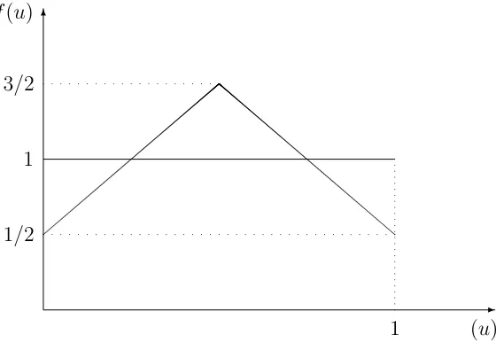
U(α1,Ω) =U(α2,Ω)∈[0,1]. The distributions of the payoffs are as shown in the following graph.

✻

✲

f(u)

(u) 1

1

1/2 3/2

For these distributions, an agent choosing action α1 is, ex-ante, equally likely to get higher or

lower utility compared to an agent choosing action α2, and vice-versa.9 Moreover, notice that the

9

P[X1> X2] = 1

R

0

P[X1> x2]f2(x2)dx2= 1/2

R

0

(1−x2)( 1

2+ 2x2)dx2+ 1

R

1/2

(1−x2)( 5

only agents who can change are those in the boundary between the groups using each action. This

boundary will be moving randomly in the form of a random walk without drift. With probability 1 4(

1 4)

will move one step to the left (right) and with probability 1₂ will stay at the same position. By standard

properties of random walks, this boundary will never diverge to infinity.

The divergence of the boundary is identical to the disappearance of one of the two actions, i.e.

convergence to a monomorphic steady state. Since we have shown that this is not possible, it means

that this network will never converge to a monomorphic steady state. In fact it will be fluctuating

continuously around zero, without ever reaching a steady state.

The negative result of the previous example does not allow us to ensure convergence to a steady

state under every structure, when at least two actions are chosen by a non-negligible share of the

population. However, there exist sufficient conditions, related to the payoff and network structure,

which can ensure it.

In the following proposition, we consider cases where all the agents have bounded neighborhoods

and that all the remaining actions are chosen by non-negligible shares of the population. These two

facts yield the initial remark that no action will disappear in finite time. Nevertheless, it is shown

that it is possible for some action to be diffused to a continuously increasing share of the population,

capturing the whole of it in the long-run. Formally, if Fk is the cumulative distribution of payoffs

associated with action αk, then:

Proposition 4.2. Consider a network with arbitrarily large population, with agents behaving under

imitate-the-best rule and having bounded neighborhoods, with upper bound D. Moreover, each of the

remaining actions, {α1, ..., αm} is chosen by a non-negligible share of the population, {s1, ...sm}. If

there exists action αk such that:

(i) Fk(u)≤[Fk′(u)]D, for all k′ 6=k, and

(ii) sk is sufficiently large,

then the network will converge, with probability one, to a monomorphic steady state where every agent

chooses action αk.

Notice that D is an exponent of F.

Our sufficient condition is weaker than first order stochastic dominance, nevertheless we have

the advantage of providing a result adequate for every network structure. The important fact in

our proof, is that the agents changing to αk are, in expectation, more than those changing from αk

to some other action. In general, this condition may depend not only on the payoff structure and

the initial share, but also on the network structure, which is something we completely disregarded

payoff structure that yields the same result, then we could again ensure convergence. This result can

become the benchmark for future research on stronger conditions for specific structures.

Moreover, it is somehow surprising that a condition as strong as first order stochastic dominance

may not be sufficient. This happens either because of the complexity of the possible network

struc-tures, or because of insufficient initial share of the action of interest. To clarify this argument, we

construct the following example.

Example 4.2. Consider the linear network described in Example 4.1. At time t = 0, there are two

actions present in the network, α1 and α2. Like before, half of the population chooses action α1 (all

the agent located at zero and to the left) and, analogously, the rest choose α2. Notice that each agent

has a neighborhood consisting of two agents apart from herself. Moreover, every period, there are only

two agents, one choosing each action, who face positive probability of changing their chosen action.

The payoffs are such that F1 < F2 (i.e. action α1 First Order Stochastically Dominates action

α2), but F1 ≥ (F2)2.10 Calling rt the number of agents who change from action α2 to action α1 we

get the following:

rt=



  

  

1 with probability p1

0 with probability p2

−1 with probability p3

FOSD ensures that p1 > p3. However, the second condition means that p1 ≤p2+p3, or equivalently

p1−p3 < 1₂. The expected value of rt will be E[rt] = (p1−p3). So, lim

τ→∞

τ P t=1

rt+s1 lim

n→∞n

= p1 −p3+s1. In

order to get diffusion of α1 we need p1−p3+1₂ ≥1, which here cannot be the case. Hence, although

α1 is FOSD compared to α2, α2 will be chosen by non-negligible shares even in the long run.

On the contrary, notice that ifF1 ≤(F2)2, then it can be the case (not necessarily) thatp1−p3 ≥ 1₂

and action α1 is diffused to the whole population.

4.2.

Unbounded Neighborhoods

In this section we drop the assumption of neighborhoods being bounded. This means that as n

grows, there exists at least one agent whose neighborhood grows as well without bounds. If

neigh-borhoods are unbounded, we cannot ensure convergence to a monomorphic steady state, even when

the diameter of the network is finite. This happens because a single agent can affect a non-negligible

share of the population, meaning that in one period an action can be spread from a finite subset of

the population to a non-negligible share of it. This means that we will have more than one actions

10

For example, letF1(u) =uandF2(u) =u

chosen by non-negligible shares of the population, which may lead the network not to converge to a

monomorphic state. We clarify the above statement with the following example. Moreover, in case

of unbounded neighborhoods, it does not hold anymore the result of Proposition 3.1, based on which

the steady state has to be necessarily monomorphic. We provide an example where a network is in

steady state and there are more than one actions present.

Example 4.3. Think of the star network (Figure 2 - One Star), that satisfies finite diameter. As

the population grows, the neighborhood of agent 1 also grows, without bounds.

3

1

4

2

k

Figure 2: One Star

Suppose there are two actions present in the network, with payoffs same as in the Example 4.1.

Initially, all the peripheral agents choose action α1, while the central agent chooses α2. It is apparent

that, as n → ∞ the probability that the central agent will change her action in the second period will

go to 1, because for n very large, for any realized payoff of the central agent, there will be at least one

peripheral agent who received higher payoff than her. However, reversing the argument, as n → ∞

the probability that every peripheral agent will receive higher payoff than the central agent goes to 0.

Then, for any realized payoff of the central agent, there will be a non-negligible share of peripheral

agents who received lower payoff than this. Hence, they will change to α2. This is because, for any

realized payoff of U(α2,·) = ˆu it holds that P r[U(α1,·)≤uˆ] =F1(ˆu)>0.

A similar argument holds in every period, leading the choice of the central agent to change

ran-domly from the second period on. This leads the network to a continuous fluctuation, where a

non-negligible share of the population chooses each action in every period. Obviously, the system will

never converge to a steady state.

We have shown that without assuming the neighborhoods to be bounded, we cannot ensure

convergence to a steady state. In the following part we provide an example where the network can

be in steady state, without this being monomorphic. This is in contrast to Proposition 3.1, where

we have shown that for finite population, steady states are necessarily monomorphic. For arbitrarily

Example 4.4. Think of the following network (Figure 3 - Two Stars), that satisfies finite diameter

and two of the agents have unbounded neighborhoods.

-3

-1

-4

-2

−k

3

1

4

2

k

Figure 3: Two Stars

Suppose there are two actions present in the network, with payoffs same as in Example 4.1. All

the agents on the left star of the figure, including the center, chooseα1 and similarly all the agents on

the right star choose α2. As ngrows, the neighborhoods of the central agents grow undoubdedly. They

get connected with more and more agents choosing the same action as them and only one choosing

differently. Hence, the probability that they will change action goes to 0, as n goes to infinity, hence

they will continue acting the same, with probability one.11 _{The peripheral agents have only one}

neighbor each, who always chooses the same action as them; so none of them will change her action

either. Concluding, this network will be in a steady state where half of the agents choose each action.

The intuitive conclusion of this observation is that groups of agents who choose the same action

and communicate almost exclusively between them can ensure the survival of this action in the

long-run, since no agent of this group ever changes her choice.

5.

Conclusion

We study a model of observational learning in social networks, where agents imitate myopically the

behavior of their most successful neighbor. We focus on identifying if an action can spread in the

whole population, as well as the conditions under which this is possible. Our analysis reveals the

different properties between finite and arbitrarily large populations.

For networks with finite population, we show that the network necessarily converges to a steady

state, and this steady state has to be monomorphic. Moreover, it cannot be ensured that the action

diffused is the most efficient. This reveals the fact that small populations are more vulnerable to

11

misguidance that can lead to the diffusion of inefficient actions. Furthermore, an action’s performance

in the initial periods, is crucial for its survival, since a sequence of negative shocks in early periods

can lead to early disappearance of the action from the population.

The results differ when the population is arbitrarily large. Under the assumption of bounded

neighborhoods, an action is necessarily diffused, regardless of its efficiency, only when it is the only

one to be chosen by a non-negligible share of the population. When more such actions exist, we

provide a sufficient condition in the payoff structure, which can ensure convergence regardless of the

network architecture. The general idea behind this result is that the diffusion of an action in a very

large network is quite hard and requires either very special structure, very large proportion of initial

adopters, or an action to be much more efficient compared to the rest.

Our sufficient condition is valuable mostly in networks where the largest neighborhood has quite

small size. This increases the importance of studying the role of network architecture, rather than the

payoff structure, when applying to network where agents have large neighborhoods. The advanced

complexity of this problem, makes it hard to deal with its general version. A very interesting

and natural extension of the present paper would be to study different payoff structures in specific

networks with importance in applied problems.

The role of central agents becomes apparent when we drop the assumption of bounded

neighbor-hoods. Even an action initially chosen by a single agent can survive in the long-run, if this agent is

observed by a non–negligible share of the population. This stresses the influential power of massively

observed agents in a society. Affecting the decision of a very well–connected agent can become very

beneficial for its diffusion.

In the present paper, we have studied some important properties of an ”imitate-the-best”

mech-anism in a social network. However, there are still crucial questions to be answered. Specifically, our

analysis refers only to long-run behavior, without mentioning neither the speed of convergence, nor

the finite time behavior of the population. Different network structures are expected to have much

different characteristics, leaving open space for future research.

6.

Appendix

Proof of Proposition 3.1. Suppose that the statement does not hold. This means that at the

steady state at least two different actions are chosen by some agent. for any structure, given that

the network is connected, there will be at least a pair of neighbors, i, j ∈ N choosing different

actions. Moreover, given that the population is finite, each one of these agents must have a bounded

If we are in a steady state, this means that agent i will never change her choice. However, because

of the common support and continuity of payoff functions, as well as boundedness of neighborhoods,

it always holds that:12

P r[U(j, ωt

j)> U(l, ωlt) : for some j ∈bi,2 and for all l ∈bi,1] =

= (1− Y

j∈bi,2

P r[U(j, ωjt)≤uˆ])

Y

l∈bi,1

P r[U(l, ωtl)≤uˆ] =

= [1−F2(ˆu)bi,2]F1(ˆu)bi,1 ≥p >0 (2)

Hence, every period agentiwill change her action with strictly positive probabilityp. The probability

that she will never change, given that no other agent in the network does so, is zero, because:

lim

t→∞ ∞ Q

t=1

(1−p) = lim

t→∞(1−p)

t_{= 0}

This leads to contradiction of our initial argument. The analysis is identical under the presence of

more than two actions. Concluding, we have shown that it is impossible for a connected network

with finite population to be in a steady state when more than one actions are still present.

Proof of Lemma 3.1. Suppose that, at period t there are at least two actions observed in the

network. Take all players i∈ N such that at

i =αk. Let Ikt ={i∈N :ati =αk} be the set of agents

who chose action αk in periodt and¬Ikt ={i∈N :a t

i 6=αk}the set of agents who did not. Also, let

Ft

k ={i ∈ Ikt :Ni ∩ ¬Ikt 6=∅}, i.e. the set of agents in Ikt who have, at least, one neighbor choosing

an action different than αk. Moreover, let the set N Fkt ={i∈ Ikt : Ni∩Fkt 6=∅and i /∈Fkt} contain

those agents who have neighbors contained inFt

k, without themselves being contained in it.

Think of the following events: ˆbt _{= {ω}t

i ∈ Ω, for i ∈ Ni,αt k = {F

t

k ∪N Fkt} : Uit(αk, ωit) ≤ uˆt},

meaning that all agents in Ni,αk get payoff lower than a certain threshold and ˆB

t_={ωt

j ∈Ω, for j ∈

Ni \Ni,αt k, where i ∈ N

t

i,αk and k

′ _{6= k : U}t

j(αk′, ωt_j) > uˆt}, meaning that all the neighbors of the

above mentioned agents who choose different action get payoff higher than this threshold.

Given that the states of nature are independent between agents, we can define a lower bound to

the probability that all agents who play αk at time t change their choice in the following period and

none of their neighbors changes to αk. We denote this event asCt. In fact, Ct ⊃ {ˆbt∩Bˆt}, because

the intersection of ˆbt _{and ˆB}t_{is a specific case included in the set C}t_{. Hence,P r(C}t_{)≥P r(ˆb}t_∩Bˆt_{) =}

P r(ˆbt_{)P r( ˆB}t_{). Notice that we impose independence between ˆb}t _{and ˆB}t_{, which holds because the}

realized payoffs are independent across agents and across periods.

12

Remark: ∀αk ∈ A and ω ∈ Ω ⇒ P r[U(αk, ω) ≤ uˆ] ∈ [bt, Bt] where bt, Bt ∈ (0,1). Hence,

P r[U(αk, ω]≤uˆt)≥bt>0 and P r[U(αk, ω)>uˆt]≥ 1−Bt>0. This is because of the full support

of U and its continuity in Ω.

Using this remark we observe that P r(ˆbt_)≥b|N

t i,αk|

t and analogouslyP r( ˆBt)≥(1−Bt)

|Ni\N_i,αkt |13_.

Hence,

P r(Ct_{)≥P r(ˆb}t_∩Bˆt_{) =P r(ˆb}t_{)P r( ˆB}t_)≥b|N

t i,αk|

t (1−Bt)

|Ni\N_i,αkt | >0

Notice that, Ct _andCt+1 _{are conditionally independent, because the realization or not ofC}t _does

not give any extra information about the realization of Ct+1_.

Let Dt

αk denote the event that, starting from period t, action αk will disappear in the next dN

periods. One of the possible histories that leads to disappearance of action αk is the consecutive

realization of the eventsCt+τ _{forτ ≥0, until all the agents who were usingα}

katthave changed their

choice. The number of periods needed depends on the structure of the network. More specifically it

is at most equal to the diameter of the network, which cannot be greater than n−1. Hence, we can

construct a strictly positive lower bound for the probability of occurrence of the event Dt αk:

P r(Dtαk)≥P r(

dN−1 \

τ=0

Ct+τ) = [

dN−1 Y

τ=1

P r(Ct+τ |Ct+τ−1)]P r(Ct)≥

≥

dN−1 Y

τ=0

b|N t+τ i,αk|

t+τ (1−Bt+τ)

|Ni\N_i,αkt+τ|

= ˙B >0.

Proof of Lemma 3.2. Denote as Kt the following set of histories:

Kt ={at time t, exactly K actions have disappeared from the network}

It is enough to show that P r(Kt+τ |(K−1)t)>0 whereτ <∞(in fact, at mostτ =dN). Using

the definition of Dt

αk from Lemma 3.1 we get:

P r[Kt+τ |(K−1)t] =

X

αk∈At

{P r[Dt+dN−1

αk |(K −1)t]} −P r[

M−K−1 [

m=1

(K+m)t+τ |(K −1)t] (3)

where M is the total number of possible actions. Namely, the above expression tells that the

probability of exactly one more action disappearing in the next τ periods equals the sum of

prob-abilities of disappearance of each action, subtracting the probability that more than one them will

13

disappear in the given time period. Analogously:

P r[(K+1)t+τ |(K−1)t] = k6=k′ X

αk,αk′∈At

{P[Dt+dN−1

αk

\

Dt+dN−1

α_k′ |(K−1)t]}−P r[

M−K−1 [

m=2

(K+m)t+τ |(K−1)t]

P r[(K+1)t+τ |(K−1)t]+P r[

M−K−1 [

m=2

(K+m)t+τ |(K−1)t] = k6=k′

X

αk,αk′∈At

P r[Dt+dN−1

αk

\

Dt+dN−1

α_k′ |(K−1)t]

But:

P r[(K+ 1)t+τ |(K −1)t] +P r[

M−K−1 [

m=2

(K+m)t+τ |(K−1)t] =P r[ M−K−1

[

m=2

(K+m)t+τ |(K−1)t]}

⇒P r[

M−K−1 [

m=2

(K+m)t+τ |(K−1)t]}= k6=k′ X

αk,αk′∈At

P r[Dt+dN−1

αk

\

Dt+dN−1

α_k′ |(K −1)t]

Hence, by equation (2):

P r[Kt+τ |(K−1)t] =

X

αk∈At

{P r[Dt+dN−1

αk |(K−1)t]} −

k6=k′

X

αk,αk′∈At

{P r[Dt+dN−1

αk

\

Dt+dN−1

αk′ |(K−1)t]}

By Lemma 3.1, we have shown that the first summation is strictly larger than zero, and we just

need to show that it is also strictly larger than the second one. Notice that the first summation is

weakly larger trivially, because for any eventsA, B, C it holds thatP r[A|C]≥P r[A∩B |C]. If the

equality was possible, this would mean that the disappearance of any action would lead necessarily to

the disappearance of another action. However, this cannot be the case because of the independence

of payoff realizations across agents. Hence we have shown that: P r[Kt+τ |(K−1)t]≥B >¨ 0, which

completes our argument.

Proof of Lemma 3.3. The event of “convergence to a monomorphic state” is the same as telling

that M −1 actions will have disappeared after T periods. One possible way of this to happen is if

one action disappears every τ =dN periods. Namely:

{(M−1)t+T} ⊃ {{(K)t+τ |(K−1)t} ∩ {(K+ 1)t+2τ |(K)t+τ} ∩ · · · ∩ {(M −1)t+T |(M−2)t+T−τ}}

However, notice that the event on the right hand side of consists of other independent events,

because the states of nature are independent across periods. Hence, recalling the result of Lemma

3.3, we construct the following relation.

Pt[(M −1)t+T]≥Pt[{(K)t+τ |(K −1)t} ∩ {(K+ 1)t+2τ |(K)t+τ} ∩ · · · ∩ {(M −1)t+T |(M −2)t+T−τ}]

=Pt[(K)t+τ |(K−1)t]Pt+τ[(K + 1)t+2τ |(K)t+τ]. . . Pt+T−τ[(M −1)t+T |(M −2)t+T−τ]

This means that the probability of convergence in finite time is strictly positive. Moreover, notice

that, for all K < M −1 ⇒ C < 1. This remark is trivial because if K = M −1, the system has

already converged, nevertheless we will use this to prove the following theorem.

Proof of Theorem 3.1. Lemma 3.3 shows us that the probability that the network will NOT

converge to a monomorphic steady state in the next T periods, given that it has not converged until

the current period, is bounded below 1. Formally:

Pt{[(M −1)t+T]c |[(M −1)t]c} ≤1−C <1

The event that the network will never converge is just the intersection of all the events where the

network does not converge after t+T periods, given that it has not converged until period t.

{The Network never Converges}={N C}=

∞ \

i=0

{[(M −1)t+(i+1)T]c |[(M −1)t+iT]c}

However, again these events are independent. Namely, the event of no convergence untilt+ 2T given

no convergence untilt+T is independent of the event of no convergence att+T given no convergence

until t: {[(M −1)t+2T]c |[(M −1)t+T]c} ⊥ {[(M−1)t+T]c |[(M −1)t]c}.

Hence, we can transform the above expression in terms of probabilities:

P[{N C}] = lim

s→∞

s

Y

i=0

P{[(M −1)t+(i+1)T]c |[(M −1)t+iT]c}

≤ lim

s→∞(1−C)

s

= 0

So, the network will converge with probability one to a monomorphic steady state.

Proof of Proposition 4.1. LetIt

k={i∈N :a t

i =αk}be the set of agents who choose αk at time

t and analogously ¬It

k = {i ∈ N : ati 6= αk} the set of agents who do not. By construction of the

problem, it holds that lim

n→∞ |It

k|

n >0, hence |I t

k| → ∞ as n → ∞. On the other hand, lim_n

→∞ ¬|It

k|

n = 0,

hence only finitely many agents do not choose αk. For the rest of the notation recall Lemma 3.1.

Notice that, every action k′ _{6= k is chosen by a finite number of agents, so the longest distance,}

Lk′, between an agent choosing k′ and the closest agent choosing k′′ 6= k′ must have finite length,

l ≤ Lk′. Hence, for all k′ 6=k, the result of Lemma 3.1 still holds, if we substitute the diameter d_N

by the maximum of all these distances, say L.

P r(Dt

α_k′)≥P r(

L

T

τ=0

Ct+τ_{) =} QL

τ=0

P r(Ct+τ _|Ct+τ−1_)≥ QL

τ=0

b|N t+τ i,α

k′|

t+τ (1−Bt+τ)

Notice, as well, the importance of the assumption for bounded neighborhoods. If this did not

hold, then we could not ensure that the above product would be strictly positive. Moreover, the

expression does not hold for the action αk. The bounded neighborhoods’ assumption can hold only

if the diameter of the network grows without bounds as n grows. Given that αk is the only action

chosen by non-negligible share of the population,Lk must also grow without bounds. Hence, for any

finite number of periods τ there exists n large enough, such that action αk faces a zero probability

of disappearance before period t+τ. More intuitively, this happens because each one of the agents

choosing a different action can affect the choice only of a finite number of agents, each period. Hence,

it is not possible that a non-negligible share of the population will stop choosing αk in a finite time

period.

Subsequently, the result of Lemma 3.2 still holds, with some appropriate modification. Namely

τ = L and P r[Kt+τ | (K −1)t, I_kt+τ 6=∅] ≥ B >¨ 0, meaning that action αk cannot disappear from

the network.

With similar reasoning, we get the modification of Lemma 3.3, which tells that there is positive

probability of convergence to a monomorphic steady state in finite time, given that action αk will

not disappear. But, this is equivalent to the case where every agent chooses action αk, denoted as

{CAk}. Formally, Pt[{CAk}]≡Pt[(M −1)t+T |Ikt+T 6=∅]≥B¨(M−K−2) =C > 0.

Finally, as in Theorem 3.1, we get a similar expression, showing that the probability that agents’

behavior will not converge to the same action, given also that action αk is still present, it is bounded

below 1. However, this is equivalent to the event of “Not converging to action αk”. This is because

action αk cannot disappear, hence if the system converges to a single action, this has to be αk.

Namely:

P[{N CAk}]≡Pt{[(M −1)t+T]c |[(M −1)t]c, Ikt+T 6=∅} ≤1−C <1

P[{N CAk}] = lim s→∞

s

Y

i=0

P{[(M −1)t+(i+1)T]c |[(M −1)t+iT]c, Ikt+T 6=∅}

≤ lim

s→∞(1−C)

s _{= 0}

Which means that the network will converge with probability one, to a monomorphic steady

state, where every agent chooses the action αk.

Proof of Proposition 4.2. Notice that the following equivalence holds: Fk(u) ≤ [Fk′(u)]D ⇔

P r(U(αk,Ω) ≥ uˆ) ≥ 1 − P r(U(αk′,Ω) ≤ uˆ)D, for all k′ 6= k and ˆu ∈ U. Before convergence

occurs, there is at least one pair of agents such that ai =αk and aj =αk′, with k′ 6=k. Condition

(i) ensures that for all the agents who observe at least one neighbor (including themselves) choosing

this holds for each agent we can construct the following variable, which we assume, in the first part

of the proof, to be a finite number. Let:

rt+1 ={#i∈N :ati+1 =αk, ati =αk′, k′ 6=k} − {#j ∈N :at+1

j =αk′, at

j =αk, k′ 6=k}

In words, this represents the difference between the number of agents changing from any action αk′

to αk, minus those that change from αk to any αk′. The expected value of r_t at each round will be,

at every time period t:

En[rt] = at

j=αk

P

i:∃j∈Ni

[p1−(1−p1)] =

at j=αk

P

i:∃j∈Ni

[2p1 −1]≥r >0, for all t

The last inequality is direct implication of condition (i) and the assumption about finiteness of rt.

Since for every agent it is more probable to change to αk, we expect that more agents will change

from other actions towardsαk than the opposite.

In order to prove convergence, we need to show that in the long-run and as the population grows

it holds that:

X

t

rt+skn →n⇔ lim n→∞ lim t→∞ P t rt

n +sk≥1 (4)

By the weak law of large numbers, applied for the population, we get with probability one:

lim

t→∞

t

P

τ=1

rτ = lim t→∞

t

P

τ=1

En[rt]≥ lim t→∞rt

Which makes equation (6) equal to:

lim n→∞ lim t→∞ P t rt

n +sk ≥

lim

t→∞rt

lim

n→∞n

+sk =r+sk≥1

The equality holds because lim

t→∞t ≡nlim→∞n. Finally, the last inequality comes from condition (ii) that

requiressk to be sufficiently large. Sufficiency depends onr, which itself depends on the distributions

of the payoffs. Obviously, the more efficient is actionαk, the smaller initial population share is needed

in order to ensure convergence.

Recall that we assumed r to be a finite number. if r is a share of the population, it is apparent

that the result still holds. Even more, the result holds without any restriction on sk, because the

References

Acemoglu, D., Dahleh, M.A., Lobel, I. & Ozdaglar, A.(2011). Bayesian Learning in Social

Networks. Review of Economic Studies, doi: 10.1093/restud/rdr004(1994).

Al´os-Ferrer, C. & Weidenholzer, S. (2008). Contagion and efficiency. Journal of Economic

Theory143, 251–274.

Apesteguia, J., Huck, S. & Oechssler, J. (2007). Imitation – Theory and experimental

evi-dence.Journal of Economic Theory 136, 217–235.

Bala, V. & Goyal, S.(1998). Learning from Neighbours.Review of Economic Studies65, 595–621.

Banerjee, A. (1992). A Simple Model of Herd Behavior. Quarterly Journal of Economics 107,

797–817.

Banerjee, A. & Fudenberg, D.(2004). Word-of-mouth learning.Games and Economic Behavior

46, 1–22.

Bigoni, M. & Fort, M. (2013). Information and Learning in Oligopoly. IZA Discussion Paper

No. 7125.

Billingsley, P.(1995). Probability and measure. John Wiley & Sons, New York.

Conley, T. & Udry, C.(2010). Learning About a New Technology: Pineapple in Ghana.American

Economic Review 100, 35–69.

Ellison, G. & Fudenberg, D. (1993). Rules of Thumb for Social Learning. Journal of Political

Economy101, 612–644.

——– (1995). Word-of-mouth communication and social learning. Quarterly Journal of Economics

109, 93–125.

Eshel, I., Samuelson, L. & Shaked A. (1998). Altruists, egoists and hooligans in a local

interaction model. American Economic Review 88, 157–179.

Fosco, C. & Mengel, F.(2010). Cooperation through imitation and exclusion in networks.

Jour-nal of Economic Dynamics and Control, doi:10.1016/j.jedc.2010.12.002

Fudenberg, D. & Levine, D., (1998).The Theory of Learning in Games, MIT Press, Cambridge,

Gale, D. & Kariv, S. (2003) Bayesian Learning in Social Networks. Games and Economic

Be-havior45, 329–346.

Jackson, M.O. (2008). Social and Economic Networks. Princeton University Press.

Jackson, M.O. & Yariv, L.(2007). Diffusion of Behavior and Equilibrium Properties in Network

Games.American Economic Review, Papers and Proceedings, 97, 92–98.

Josephson, J. & Matros, A. (2004). Stochastic imitation in finite games.Games and Economic

Behavior 49, 244–259.

Lopez-Pintado, D. (2008). Contagion in Complex Networks. Games and Economic Behavior 62,

573–590.

Morris, S. (2000), Contagion,The Review of Economic Studies 67, 57–78.

Schlag, K. (1998). Why imitate, and if so, how? A boundedly rational approach to multi-armed

bandits.Journal of Economic Theory 78, 130–156.

——– (1999). Which one should I imitate? Journal of Mathematical Economics 31, 493–522.

Weibull, J. (1995). Evolutionary Game Theory. MIT Press, Cambridge, MA.