Terrain Details Effect on Connectivity in Ad hoc Wireless Networks

Terrain Details Effect on Connectivity in Ad hoc

Wireless Networks

Sonja Filiposka, Igor Mishkovski, Blanka Taslamicheska Trajkoska Faculty of Computer Science and Engineering, Ss. Cyril and Methodius University, Skopje, R. Macedonia

Email: sonja.filiposka@finki.ukim.mk, igor.mishkovski@finki.ukim.mk, taslamiceska@gmail.com

Received 2013

ABSTRACT

In this work, we conduct a research on the effects of the details of the terrain on the path establishment in wireless net-works. We discuss how the terrain induced variations, that are unavoidably caused by the obstructions and irregularities in the surroundings of the transmitting and the receiving antennas, have two distinct effects on the network. Firstly, they reduce the amount of links in the network connectivity graph causing it to behave more randomly, while decreasing the coverage and capacity of the network. Secondly, they increase the length of the established paths between the nodes. The presented results show how the terrain oblique influences the layout of the network connectivity graph, in terms of different network metrics, and gives insight to the appropriate level of details needed to describe the terrain in order to obtain results that will be satisfyingly accurate.

Keywords: 3D Terrain Aware Propagation; Network Connectivity Graph; Path Length Distribution

1. Introduction

Propagation models for wireless networks have tradi-tionally focused on predicting the average received signal strength at a given distance from the transmitter, as well as the variability of the signal strength in proximity to a particular location. Typically, when estimating the ad hoc network performances very little attention is given to the terrain [1], and thus, to the propagation model used for the estimation [2-4]. The nodes are assumed to be scat-tered on a flat, regular terrain and a simple ground reflec-tion propagareflec-tion model is used.

However, radio transmission in a mobile communica-tions system often takes place over irregular terrain. Since terrain irregularities can greatly affect and distort the expected network performances, great care must be taken when trying to reflect the real-life use of the mod-eled network. Therefore, the terrain profile of a particular area needs to be taken into account when estimating the path loss since the transmission path between the trans-mitter and the receiver can vary from simple line-of-sight to one that is obstructed by buildings, hillsides or foliage. In this paper we investigate the influence of the terrain detail level on the network connectivity, coverage and capacity for a typical ad hoc network simulation. Fur-thermore, we investigate how the different detail level of the terrain influences the layout of the network connec-tivity graph, especially in terms of network partitioning, average path length, node degree distribution and similar

metrics from graph theory. Additionally, using 3D terrain wireless simulations in NS-2 we study the influence of the network connectivity graph changes on the multi-hop path establishment and network performances.

The results from this paper are intended to show how the terrain can increase the average path length, while also increasing the overall network performances, be-cause of the possibility of increased number of parallel radio transmissions. The results help the user to choose the appropriate level of details for a given terrain in order to obtain more realistic results with faster simulations.

The rest of this paper is organized as follows: Section 2 is an introduction to terrain aware propagation and the terrain model. In Section 3 we use metrics from graph theory to analyze the changes in the network connectivity. Section 4 presents analyses of the performances of the case study ad hoc network over 3D terrains with different detail level. Finally, Section 5 concludes this paper.

2. Terrain Aware Propagation Models

Another interesting implementation is the AMADEOS extension [6] to NS-2 and Glomosim[7]. In addition to the developed mobility models, it provides a ray-tracing routine combined with a geometry DXF file that de-scribes environment characteristics. The algorithm is based on a 2D ray tracing technique and is more than seven times slower than the two-ray ground simulations.

The OPNET's Terrain Modeling Module (TMM) [8] also adds Earth topology, such as mountains, forests and valleys, as well as user-selectable environmental condi-tions to the simulated network model. There are several terrain aware propagation models that are included: the Longley-Rice model [9], TIREM [10] and the Wal-fisch-Ikegami model [11]. TMM imports and graphically displays elevation information from Digital Terrain Ele-vation Data (DTED) and the US Geological Survey Digital Elevation Maps (USGS DEM) formats, enabling accurate calculation of signal strength.

In this paper a similar approach to TIREM is used. The 3D terrain aware propagation model used is a Durkin’s extension based on knife edge diffraction for the open source NS-2 [12]that will provide the users with the abil-ity to add terrains into triangular irregular network (TIN) format.

The TIN model is one of the most common vec-tor-based models of surface. It represents a surface as a set of contiguous, non-overlapping triangles. Within each triangle the surface is represented by a plane. The trian-gles are defined with a set of points called mass points. These mass points can occur at any location, the more carefully selected, the more accurate the model of the surface. A TIN-based model is able to describe features very well. Although grid based DEMs are easy to handle, triangulated irregular network models (TINs) have be-come increasingly popular for the representation of ter-rain surfaces because of their ability to accommodate irregularly spaced elevation data. It enables them to adapt to the variable complexity of the relief and to integrate structural features (breaklines, ridges, ...) in the terrain model [15]. A diversity of TIN-based interpretation pro-cedures is already available today. It has been shown that many of these procedures have clear advantages over their grid-based counterparts [16,17].

Since the TIN format needs less data to represent the terrain, the simulations are a lot faster compared to the DEM based solutions. TIN also offers another opportu-nity for the user, i.e. adaptable detail level of the terrain description by changing the level of mean or max error. The lower the detail level, i.e. the number of triangles, the bigger the RSME and max error, but, on the other hand, the simulations run faster. In order to get a more clear picture how the RSME and max error change when the number of triangles is increased, we have generated a great deal of different representations of one example

TIN terrain. Table 1 summarizes some of the obtained results for one example terrain with size 1000 x 1000 m, where the mean height is 783.20 m and the standard de-viation to this value is 19.93 m (hilly terrain).

As it is shown in Table 1 the error is rapidly decreased with the increased number of triangles up to a certain point. We discovered that when the max error is less than 1 m, i.e. for more than 4000 triangles, the terrain repre-sentation is quite acceptable for graph theory analysis or network simulations. Adding more than 12456 triangles does not improve the terrain accuracy, because the rep-resentation is an exact match to the real life terrain.

3. Graph Connectivity Analysis

In order to investigate the essential properties of ad hoc networks, such as connectivity and degree distribution, one needs realistic modeling. This Section is dedicated to better understand how the fundamental properties change in different environment and analyzes the prerequisite for reliable user application connections in the network.

The analysis of coverage and connectivity in wireless ad hoc networks modeled using 3D terrains and suitable propagation model can be addressed using tools and re-sults from graph theory.

Network connectivity has been an active research topic in the scientific community. Hekmatand and Mieghem in [18] have studied connectivity in wireless ad hoc net-works when using statistically variable radio signal power. Barrett et al. in [19] focused on the computation of the connectivity graph for large networks and explore approximation alternatives to compute graph connec-tivity by examining different graph metrics. In [20], Miorandi and Altman present an analytical procedure for computing the node isolation probability in presence of channel randomness. However, in our work instead of using random statistical variables we analyze the connec-tivity using radio propagation model that is based on knife edge diffraction that occurs because of terrain ob-stacles.

A wireless ad hoc network consists of a number of wireless nodes scattered over a certain geographic area. Every node may be connected to other nodes in its vicin-ity. We assume that connections between nodes are two- way, undirected links. At any instant in time an ad hoc

Table 1. Statistical data on tin terrain accuracy.

# triang. RSME _error max mean _{error height} min _height max

12456 0.00 0.00 0.00 741.00 830.33

4000 0.30 0.75 0.21 741.00 830.00

200 2.18 7.31 1.69 741.67 821.67

network can be considered as a graph with a fixed topol-ogy. The actual set of connections depends on the geo-metric distance between nodes. Graphs with distance- dependent links between nodes and correlated links are referred to as random geometric graphs [21].

When assuming a flat terrain, the network connectivity graph is a random geometric graph, wherein each node has a transmission range represented as circle with a fixed radius. However, when considering the terrain ef-fect on propagation, this is no longer true and prevents us from continuing to use the random geometric graph ap-proach. When taking into account the terrain features, a number of nodes will no longer be able to communicate directly due to obstacles existing between them. How-ever, in special cases, there could also be newly estab-lished links because of the effects of the diffraction. Fig-ure 1 presents the network connectivity graph for 100 uniformly randomly scattered wireless ad hoc nodes on a flat terrain. This number of nodes is chosen so that for the given network area size (1000 x 1000 m) and as-sumed flat terrain, the randomly scattered nodes always form a connected graph. Figure 2 shows how the con-nectivity changes in presence of terrain. The network connectivity graph is obtained by calculating the radio coverage of each node in the network by using the terrain aware propagation model. When comparing the two connectivity graphs, we observe that the terrain induces a certain level of ‘localization’ or grouping of the nodes according to their vertical positioning (height). There are also two completely ‘dark’ unconnected nodes (node ID 90 - upper left and node ID 82- lower right corner). Fur-thermore, the network connectivity graph is sensitive to the number of triangles used to describe the terrain.

We have applied different graph theory metrics in or-der to measure the changes of the network connectivity graphs. The results shown in Table 2 confirm that using a terrain representation with max error less than 1m gives almost identical results as using maximum number of triangles (i.e. 12456 triangles). As the number of trian-gles increases the network density (i.e. the number of edges and average node degree) decreases. As a conse-quence, the average and the maximum distance between the nodes are increased. Please note that these values are calculated for the reachable nodes only. The most distant nodes (in terms of number of hops) are always located at the opposite edges of the terrain, as it is expected. It is interesting to note that even for a small number of trian-gles (beginning from 20 in our case) the network is fragmented in several partitions increasing the number of unreachable paths. The number and the structure of the partitions are strongly influenced by the terrain oblique. For our example terrain represented with more than 20 triangles the network is partitioned in five clusters (two of which have only one node, the others have 4, 12 and

the giant componentsize equals to 82 nodes). The only case in which we did not observe network partitioning is when using 10 triangles to represent the terrain features; however, this representation is far from accurate (see

Table 1).

Figure 1. Connectivity graph for an example ad hoc network on a flat terrain.

Figure 2. Connectivity graph for an example ad hoc network on a TIN terrain based on 4000 triangles (minheight deep green –max height white).

Table 2. Connectivity graph changes due to terrain effects.

Flat with terrain aware 3D propagation # triang.

Metric

0 10 200 4000 12456

In connected graphs there is a natural distance metric between all pairs of nodes, defined by the length of their shortest paths. Thus, the more central a node is, the lower its total distance to all other nodes. Closeness can be re-garded as a measure of how fast it will take to send in-formation from one to all other nodes sequentially [18].

Figure 3 shows the closeness centrality value for all the nodes in the network for the terrain represented with dif-ferent number of triangles. In the case of flat terrain (i.e. the number of triangles is 0) the nodes are more central, i.e. the distance from any node to all other nodes is small. Whereas, in the case of high resolution terrain descrip-tion (using 12456 triangles) the nodes are further apart from each other, i.e. they have greater closeness value.

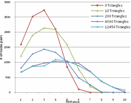
In Figure 4 we plotted some results in terms of dis-tance distribution for various numbers of triangles used to represent the terrain. It can be concluded that in all cases the prevalent distances in the network are remain-ing to be 3 and 4 hops long. The introduction of the ter-rain decreases their frequency while increasing the num-ber of longer paths. We again confirm that choosing a terrain that is represented by more than 4000 triangles (less than 1m max error) does not influence the distance distribution.

4. Network Performance Analysis

In the previous Section we have analyzed network con-nectivity graph independently from the traffic load in the network. On the physical layer, connectivity between nodes is predicted by the radio propagation model. Whether two connected nodes can communicate with each other also depends on the interference condition which is directly linked to parallel communication be-tween other nodes in the network. Due to interference, communication between two connected nodes may even

Figure 3. Closeness centrality for the connectivity graph with a different terrain detail level

Figure 4. Distance distribution for the connectivity graph with a different terrain detail level.

become impossible at certain moments. Thus, interfer-ence can be considered as a capacity-affecting factor. This Section investigates the changes of the interference induced network connectivity between the nodes.

The primary objective of our case study simulations is to understand the impact of the amount of details used to represent the terrain in a simulation environment for wireless ad hoc networks. In this Section we investigate the aspects of traffic throughput, average path length of the received network traffic, distance distribution for the received and dropped network traffic and the average routing load of the nodes for the Durkin’s propagation model using TIN files with different level of details. For the case study evaluations made in this paper, we decided to work with a number of real terrains, but since the ob-tained result trends are statistically equal, here we present the results for the real terrain given in Figure 2.

The terrain is described by a number of TIN files from 10 to 12456 triangles. The complete ad hoc network of 100 nodes all equipped with an IEEE 802.11b radio and a transmission range of 250 m. The nodes are uniformly scattered in the terrain area. The routing protocol used is AODV [23]. The traffic pattern is a completely random traffic between the nodes with the offered traffic of 3Mbps. We created one scenario for each terrain repre-sentation with a different detail level based on the num-ber of triangles. It was crucial that the traffic pattern and positioning pattern scenarios are defined only once and are used for all the terrains so that the differences in the results are exclusively due to the terrain discrepancies. The results shown here are averaged over the results ob-tained for 10 different generated scenarios.

using more triangles (for which we are sure that the maximum error is less than 1 m), the obtained results are converging to the same value. However, it is more inter-esting to conclude that even for a lesser number of trian-gles the results can still be taken into consideration with some skeptics in mind. As it is shown, for terrains with more than 400 triangles the results fit within a close range. Given that the simulations are many times faster when the number of triangles is smaller, with regards to

Table 1, we can conclude that in cases when we need fast first order approximation we can use terrains that are generated with a relatively small number of triangles.

When using flat terrain the end-to-end received traffic is around 8.2%, which is 2 times less compared to the case when using 12456 triangles to represent the terrain. This is due to the fact that the obstacles between the nodes allow multiple parallel transmissions to occur.

The average path length of the received network traffic for the example ad hoc network is presented in Figure 6. The presence of the terrain drastically increases the av-erage path length. However, the amount of detail levels does not increase it on a large scale. The relative increase in average path length is equal for the connectivity graph (see Table 2) and for the simulated network results, valuing around 60%.

The influence of the increased average path length is shown in more details in Figure 7, which represents the distance distribution for the received network traffic for the example ad hoc network on a different terrain detail level. Most of the received network traffic for the flat terrain is due to one hop-direct communication. In the case of using terrains the amount of one-hop received traffic decreases, while most of the received traffic is sent by 2 or 3 hops. Furthermore, for the flat terrain al-most all of the received traffic is transmitted via less than 6 hops. Another important result is that most of the dropped traffic occurs at the sender. This means that

Figure 5. Received traffic of the offered traffic for the exam-ple ad hoc network on a different terrain detail level.

while the packets wait in the queue, the sender is not able to find a suitable route to the destination and because of the high amount of sending traffic the queue keeps in-creasing and eventually starts to drop packets.

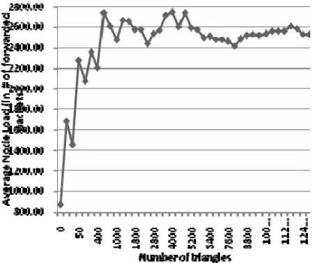
The average node load in terms of forwarded packets for the example ad hoc network is shown in Figure 8. We calculate the average node load as the number of packets one node has forwarded acting as a router in a multi-hop path. Keep in mind that this does not always mean that the end-to-end connection was successful. The packet may have been dropped further along the route.

In the case of flat terrain most of the traffic is received only by one hop and the ad hoc network nodes are under drastically lesser load compared to the terrain aware simulation scenarios. However, similar to the case of average path length and the percentage of received traffic, the increased amount of detail levels does not induce more routing load to the nodes on a large scale.

Figure 6. Average Path Length for the received network traffic on a different terrain detail level.

Figure 8. Average node load for the received network traffic on a different terrain detail level.

5. Conclusions

In this paper we have presented an analysis of the influ-ence of the terrain detail level on the path establishment in wireless ad hoc network by exploring the changes in the network connectivity graph. We have also investi-gated the difference of the obtained results compared to the behavior of a wireless ad hoc network deployed on a flat terrain. The main conclusion is that the terrain de-creases the number of links between the nodes, which leads to longer paths and network partitioning. However, this does not necessarily mean lower performance. On contrary, the obstructions between the nodes can allevi-ate the interference and, in some cases, improve the net-work performances. Another goal of this net-work was to determine the amount of terrain detail necessary to obtain satisfyingly accurate results. The results show that when using relatively small number of triangles to represent the terrain, the network behavior is close to the most de-tailed scenario, while the simulation runs several times faster.

REFERENCES

[1] C. M. Lee, V. Pappas, S. Sahas and S. Seshan, “Impact of Coverage on the Performance of Wireless Ad Hoc Net-works,” Proceedings of the Second Annual Conference of the International Technology Alliance, UK, 2008. [2] K. O. Tonguz and G. Ferrari, “Ad Hoc Wireless

Net-works: A Communication-Theoretic Perspective,” John Wiley & Sons, 2006.doi:10.1002/0470091126

[3] W. Shan, W. Jian-xin, Z. Xu-dong and W. Ji-bo, “Per-formance of Anti-jamming Ad Hoc Networks Using Di-rectional Beams with Group Mobility,” FIP International Conference on Wireless and Optical Communications Networks, 2006.

[4] R. aumann, S. eimlicher and M. May, “Towards Realistic Mobility Models for Vehicular Ad-hoc Networks,”26th Annual IEEE Conference on Computer Communications, Alaska, USA, 6-12 May 2007.

[5] R. Vuyyuruand and K. Oguchi, “Vehicle-to-vehicle Ad Hoc Communication Protocol Evaluation Using Realistic Simulation Framework,” Wireless on Demand Network Systems and Services, 2007, Fourth Annual Conference on WONS '07, 2007.

[6] A. -K. Harouna, Souley and S. Cherkaoui, “Realistic Urban Scenarios Simulation for Ad Hoc Networks,”The Second International Conference on Innovations in In-formation Technology (IIT’05), 2005.

[7] Glomosim, “Global Mobile Information Systems Simula-tion Library,” http://pcl.cs.ucla.edu/projects/glomosim/

[8] OPNET Modeler Wireless Suite,

http://www.opnet.com/solutions/network_rd/modeler_wir eless.html.

[9] G. Hufford, “The ITS Irregular Terrain Model,” http://flattop.its.bldrdoc.gov/itm.html.

[10] TIREM specifications,

http://www.alionscience.com/Technologies/Wireless-Spe ctrum-Management/TIREM/Specifications.

[11] W. Ikegami, “Cost 231 - Cost Final Report,” http://www.lx.it.pt/cost231/.

[12] “NS-2 network simulator,” http://nsnam.isi.edu/.

[13] M. Vuckovik, S. Filiposka and D. Trajanov, “Perform-ances of Clustered Ad Hoc Networks on 3D Terrains,” SIMUTools ’09, Rome, Italy, 2009.

[14] S. Filiposka and D. Trajanov, “Terrain Aware 3D Radio Propagation Model Extension for NS-2,” Simulation Journal, 2011.

[15] R. Weibel and M. Heller, “Digital Terrain Modeling,” In: Geographical Information Systems: Principles and Ap-plications, London: Longman, 1991, pp. 269-297.

[16] M. F. Goodchild and J. Lee, “Coverage Problems and Visibility Regions on Topographic Surfaces,” Annals of Operations Research, Vol. 18, 1989, pp. 175-186. doi:10.1007/BF02097802

[17] B. Falcidieno and M. Spagnuolo, “A New Method for the Characterization of Topographic Surfaces,” International Journal of Geographical Information Systems, Vol. 5, No. 4, 1991, pp. 397-412.

doi:10.1080/02693799108927865

[18] R. Hekmat and P. V. Mieghem, “Study of Connectivity in Wireless Ad-hoc Networkswith an Improved Radio Model,” Proceedings of WiOpt, Cambridge, UK, 2004.

[19] C. L. Barrett, M. V. Marathe, D. C. Engelhart and A. Sivasubramaniam, “Approximate Connectivity Graph Generation in Mobile Ad Hoc Radio Networks,” 36th Annual Simulation Symposium, 2003, pp. 81-88.

[21] M. Penrose, “Random Geometric Graphs,” Oxford Uni-versity Press, New York, 2004.

[22] M. E. J. Newman, “A Measure of Betweenness Centrality Based on Random Walks,” Social Networks, Vol. 27,

2005, pp. 39-54.doi:10.1016/j.socnet.2004.11.009