BIROn - Birkbeck Institutional Research Online
Hu, W. and Hu, R. and Xie, N. and Ling, H. and Maybank, Stephen J. (2014)
Image classification using multiscale information fusion based on saliency
driven nonlinear diffusion filtering. IEEE Transactions on Image Processing
23 (4), pp. 1513-1526. ISSN 1057-7149.
Downloaded from:
Usage Guidelines:
Please refer to usage guidelines at or alternatively
Image Classification Using Multi-Scale Information Fusion
Based on Saliency Driven Nonlinear Diffusion Filtering
1
Weiming Hu, Ruiguang Hu, and Nianhua Xie
(National Laboratory of Pattern Recognition, Institute of Automation, Chinese Academy of Sciences, Beijing 100190) {wmhu, rghu, nhxie}@nlpr.ia.ac.cn
Haibin Ling
(Department of Computer and Information Science, Temple University, Philadelphia, USA) [email protected]
Stephen Maybank
(Department of Computer Science and Information Systems, Birkbeck College, Malet Street, London WC1E 7HX) [email protected]
Abstract: In this paper, we propose saliency driven image multi-scale nonlinear diffusion filtering. The resulting
scale space in general preserves or even enhances semantically important structures such as edges, lines, or flow
like structures in the foreground, and inhibits and smoothes clutter in the background. The image is classified
using multi-scale information fusion based on the original image, the image at the final scale at which the
diffusion process converges, and the image at a mid-scale. Our algorithm emphasizes the foreground features
which are important for image classification. The background image regions, whether considered as contexts of
the foreground or noise to the foreground, can be globally handled by fusing information from different scales.
Experimental tests of the effectiveness of the multi-scale space for image classification are conducted on the
following publicly available datasets: the PASCAL 2005 dataset, the Oxford 102 flowers dataset, and the Oxford
17 flowers dataset, with high classification rates.
Index terms: Saliency detection, Nonlinear diffusion, Multi-scale information fusion, Image classification
1. Introduction
Image classification [35] is a very active research topic which has stimulated researches in many important
areas of computer vision, including feature extraction and feature fusion [1, 24], the generation of visual
vocabulary [32], the quantization of visual patches to produce visual words [25, 28], pooling methods [32], and
classifiers [22].
In image classification, it is an important but difficult task to deal with the background information. The
background is often treated as noise; nevertheless, in some cases the background provides a context, which may
increase the performance of image classification. Zhang et al. [33] experimentally analyzed the influence of the
1
background on image classification. They demonstrated that although the background may have correlations
with the foreground objects, using both the background and foreground features for learning and recognition
yields less accurate results than using the foreground features alone. Overall, the background information was
not relevant to image classification. Heitz and Koller [10] showed that spatial context information may help to
detect objects. Shotton et al. [21] proposed an algorithm for recognizing and segmenting objects in images, using
appearance, shape, and context information. They assumed that the background is useful for classification and
there are correlations between foreground and background in their test data. Galleguillos et al. [5] proposed an
algorithm that uses spatial context information in image classification. The input image was first segmented into
regions and each region was labeled by a classifier. Then, spatial contexts were used to correct some of the labels
based on object co-occurrence. The results show that combining co-occurrence and spatial contexts improves the
classification performance. From the previous work, we conclude that image classification is faced with the
partial matching problem [8, 14]: some features obtained from images in the same class differ significantly from
one image to another because of background clutter and occlusion of the foreground objects by other objects.
The influence of background on image classification varies. Only semantically important contexts, such as object
co-occurrence, or particular object spatial relations are helpful for image classification. Backgrounds which
contain only clutter provide no information to support image classification. It is interesting to filter out
background clutter and simultaneously use the background context to increase the performance of image
classification.
In order to deal effectively with the background information, we propose a saliency driven nonlinear
diffusion filtering to generate a multi-scale space, in which the information at a scale is complementary to the
information at other scales.The fusion of information from different scales may improve the image classification
performance. A nonlinear diffusion [29, 41, 42, 43, 44], which has been widely used in image denoising,
enhancement, etc, can preserve or even enhance the semantically important image structures, such as edges and
lines. However, nonlinear diffusion treats the foreground and the background equally. Most annotated images
contain subjects that are highly likely to be salient regions. Background regions and foreground regions can often
be identified using the image saliency: for example, a photographer usually and naturally assigns more saliency
to foreground regions. Saliency detection techniques [7, 9, 12, 16, 23, 27], which are currently popular, can be
used to estimate the foreground and background regions according to the saliency distribution. Background
clutter is for the most part filtered out, while foreground features are preserved. We combine a saliency map,
saliency map to define the weights of image gradients. During the diffusion process, the image gradients in the
salient regions are increased while those in non-salient regions are decreased. Accordingly, when the scale
increases, the background information gradually fades out while the foreground information is preserved and
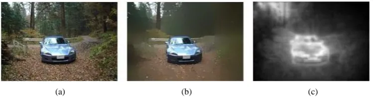
important structures in the foreground are enhanced. Figure 1 shows an example of the saliency driven nonlinear
diffusion filtering. It is clear that, based on the saliency map, the background regions corresponding to
non-salient regions are smoothed, and the foreground car, corresponding to salient regions with important image
structures, is preserved. After saliency driven nonlinear diffusion, an image is represented by the set of its
multi-scale images. Information fusion is carried out in the nonlinear multi-scale space to improve the
performance of image classification.
[image:4.595.112.487.286.384.2](a) (b) (c)
Figure 1. An example of saliency driven diffusion filtering: (a) The original image; (b) The image after diffusion; (c) The saliency
map.
The saliency driven multi-scale space of an image can be used to handle uncertain background information.
As shown in Figure 1, at large scales, the background is filtered out and the foreground is preserved. At small
scales, background and foreground regions are both preserved. If the background is a context of the foreground,
the images from the same class may be more similar at small scales than at large scales. If the background is
clutter, then images from the same class are more similar at large scales than at small scales. We use the
weighted average of the distances at some representative scales to represent the dissimilarity between different
images. The weighted average is preferred to the minimum of the distances at all the scales because the risk of
incorrectly filtering is less. Using this multi-scale representation, background information can be effectively
dealt with.
This saliency driven nonlinear multi-scale image representation has several advantages:
In the nonlinear scale space, semantically important image structures are preserved or enhanced at
large scales, and the locations of the important image structures are not shifted after diffusion at any
scale. This differs from the Gaussian scale space in which parts of important image structures may be
smoothed and detected edges are shifted from their true locations after Gaussian convolution.
matter whether the background is a context for the foreground or is only noise as far as the foreground
is concerned.
This saliency driven nonlinear multi-scale representation can be easily supplied as input to any existing
image classification algorithms, e.g., bag-of-words.
The rest of the paper is organized as follows. Section 2 proposes the saliency driven nonlinear diffusion
filtering. Section 3 discusses the estimation of the diffusion parameters. Section 4 presents the saliency driven
multi-scale information fusion. Section 5 shows the experimental results. Section 6 concludes the paper.
2. Saliency Driven Nonlinear Diffusion
We first give a brief review of linear and nonlinear diffusion filtering [29], and saliency detection
techniques. Then, we propose our saliency driven nonlinear diffusion filtering.
2.1. Linear and nonlinear diffusion filtering
2.1.1. Linear diffusion and Gaussian scale space
Let
u x y t
( , , )
be the grey value at position( , )
x y
and scale t in the multi-scale space. The imagediffusion filtering is defined by the diffusion equation [29]:
(
)
(
)
t
u
div D
u
D
u
(1)where is the gradient operator: ( / x, / y), “div” is the divergence operator, and D is the diffusion
tensor which is a positive definite symmetric matrix. If D is defined as a constant over the whole image domain,
then (1) is the homogeneous diffusion equation which corresponds to the Gaussian scale space, otherwise it
corresponds to a position-dependent filtering which is called inhomogeneous diffusion.
For the homogeneous linear diffusion filtering, Equation (1) reduces to
( , , 0)
( , )
t
u
u
u x y
f x y
(2)where f x y( , ) is the original image and u u. Let
K
be a Gaussian with the standard deviation
:2 2
2 2
1
( , )
exp(
)
2
2
x
y
K
x y
. (3)The solution of (2) is a convolution integral:
1 2 1 2 1 2
2 2
( , , )
t( , )* ( , )
t( ,
) (
,
)
(
0)
u x y t
K
x y
f x y
K
f x
y
d d
t
(4)is the so-called Gaussian scale space. The Gaussian smoothing not only reduces noise, but also blurs important
image structures, such as edges. Thus, the features extracted from images at large scales are not suitable for
image classification.
2.1.2. Nonlinear diffusion
If the D in (1) is a function
g
(
u
)
of the gradient
u
of the evolving image u itself, then Equation (1)defines a nonlinear diffusion filter [20, 29]. The function
g
(
u
)
is usually defined as:2 2
1
(
)
(
0)
1
D
g
u
u
(5)where
is a predefined parameter. The nonlinear diffusion filtering is represented as:(
)
( (
)
)
t
u
div D
u
div g
u
u
. (6)The regions in which
u
are blurred, while the other regions are sharpened. The nonlinear diffusionpreserves and enhances image structures defined by large gradient values. If image structures with large
gradients are all in the foreground, nonlinear diffusion filters out the background. However, there may be large
image gradients in the background. Thus, we propose a saliency driven nonlinear diffusion equation which blurs
non-salient regions and preserves salient regions.
2.2. Saliency detection
Saliency detection methods can be grouped into supervised and unsupervised. In the following, we first
introduce the supervised methods and then the unsupervised methods. Finally, the method used in this paper is
introduced.
Supervised methods [37, 38] detect saliency using a classifier which is trained using samples for which
saliency is well labeled. Marchesotti et al. [17] trained a classifier for each target image using the images most
similar to it in an annotated database to construct its saliency map. The underlying assumption is that images
sharing a globally similar visual appearance are likely to share similar saliencies. This supervised saliency
detection needs a very large well-labeled image database, which is not easy to obtain.
Unsupervised saliency detection [39, 40] usually starts with features of image structures known to be salient
for the human visual system (HVS). These structure features include the intensity of salient regions, and the
orientation, position and color of edges. Goferman et al. [7] summarized the following three principles for
saliency detection by the HVS:
Frequently occurring features should be suppressed [11, 16, 23].
The salient pixels should be grouped together, rather than scattered across the image.
The characteristic of Goferman’s method is that the regions that are close to the foci of attention are explored
significantly more than far-away regions. As a result, some background regions near to the salient structures are
included in the saliency map, but foreground regions are rarely incorrectly classified as background regions. The
limitation of Goferman’s method is that it often produces high values of saliency at the edges of an object but
lower saliency within the object. Cheng et al. [34] proposed a histogram-based contrast method to measure
saliency. Their algorithm separates a large object from its surroundings, and enables the assignment of similar
saliency values to homogenous object regions, and highlights entire objects.
In our work, we take advantages of Goferman’s method and Cheng’s method by averaging the two saliency
maps obtained using these two methods to form the saliency map that we use. The edges and the interiors of the
foreground objects tend to have comparatively high saliency values. In this way, the saliency map tends to
include as much foreground as possible.
2.3. Saliency driven nonlinear diffusion
We combine a saliency map as priori knowledge with nonlinear diffusion filtering. Let
I
s be the saliencymap. To introduce the saliency information into the diffusion process, we combine
I
s into D in (6) and defineD as a function g of
u
andI
s. Then, the diffusion equation becomes( , , )
( , )
0
( (
,
)
)
0
t s
u x y t
f x y
if t
u
div g
u I
u
if t
. (7)We define the diffusivity
g
(
u I
, )
s as:1 exp
0
(
,
)
1
0
s m s s sC
if I
u
g
u I
I
u
if I
u
(8)where
C
is a constant,
is the contrast parameter, and m controls the speed of the diffusivity [3, 30]. Weexplain the following points with respect to (8):
We propose to apply
I
s directly to the norm of the gradient
u
, such thatI
s works as a maskThen, when
I x y
s( , ) 1
, the effect of the gradient at (x,y) is increased during the diffusion process,otherwise it is suppressed.
The flux
g
(
u I
, )(
sI
s
u
)
increases asI
s
u
increases ifI
s
u
and decreases as
s
I
u
increases ifI
s
u
. If
u
is less than
, then the flux increases when
u
increases, otherwise the flux decreaseswhen
u
increases. The larger the value of the parameter m, the more quickly the flux changes in response to changes in
s
I
and
u
. When
I
s
u
is very large, the diffusion function value approximates 0. WhenI
s
u
is verysmall, it approximates 1.
The optimization of the parameters C, , and m is presented in Section 3.
The above saliency driven nonlinear diffusion filtering can be used directly only for gray images. For color
RGB images, there is a single application in which the gradients from the RGB channels are combined: the
diffusion filtering is applied to the 2 norm of the gradients obtained from the three channels. This use of all
[image:8.595.147.448.488.658.2]the three channels smooths out errors from the RGB channels.
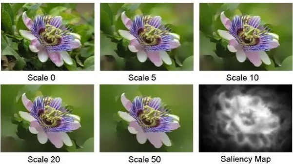
Figure 2. Different scales for an example image and its saliencymap: the scale number corresponds to t in (7).
Figure 2 shows an image at different scales and its saliency map. It is seen that our saliency driven
nonlinear diffusion leads to image simplification in the non-salient region, i.e. most of the structures in this
region are blurred and smoothed. In the salient region, the evolution of scales preserves or even enhances
nonlinear diffusion with the result of nonlinear diffusion omitting the saliency map at scale 10. It is clearly seen
that the background regions are smoothed more effectively by using saliency information, while the foreground
regions are preserved. The images produced by our saliency driven nonlinear diffusion are more suitable for
image classification than those produced by normal nonlinear diffusion. Although these examples are taken from
static background and still images, our work can be adapted to time-varying background from moving platforms,
[image:9.595.217.380.210.434.2]because our saliency driven nonlinear diffusion filtering can effectively deal with the background information.
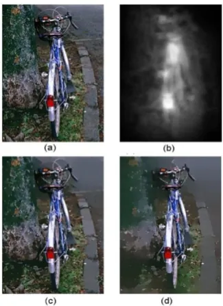
Figure 3. An example of comparison between non-linear diffusion and saliency driven nonlinear diffusion: (a) The original image;
(b) Saliency map; (c) Nonlinear diffusion at scale 10; (d) Saliency driven nonlinear diffusion at scale 10.
3. Estimation of Diffusion Parameters
The optimization of the parameters C,
, and m in (8) is important for our saliency driven nonlineardiffusion filtering. In the following, we first discuss the properties of these three parameters, and then give a
method for determining their values.
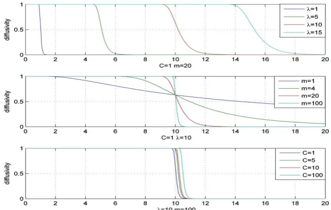
Figure 4 shows the diffusivity function values for different values of the parameters, where the horizontal
coordinate is the value of
I
s
u
, and the vertical coordinate is the value of the diffusivity. Figure 5 shows thediffusion results for different values of
and m. Referring to Figures 4 and 5, we make the following pointsabout the three parameters:
1) In the nonlinear diffusion filtering, the parameter
plays an essential role as a threshold parameter.Structures with
are regarded as edges, where the diffusivity is close to zero, while structures with
smoothes the interiors of regions but preserves their edges [26]. As shown in Figure 5, when
is too small,neither the foreground nor the background are smoothed; when
is too large, both the foreground and thebackground are smoothed; when
is appropriately chosen, the background is smoothed and the foreground ispreserved. As shown in the top subfigure in Figure 4, it is difficult to directly set an empirical value to
. It isnecessary to choose an appropriate value of
for each image, in order to maintain the performance of the [image:10.595.129.465.214.427.2]algorithm.
Figure 4. The diffusivity function values for different values of the parameters: The top subfigure shows the changes in diffusivity
values when
increases, and m and C are fixed; The middle subfigure shows the changes in diffusivity values when m increases,and
and C are fixed; The bottom subfigure shows the changes in diffusivity values when C increases, and
and m are fixed.Figure 5. The diffusion results with different values of the parameters: The first row shows the original image and the saliency mask; The second row shows, from the left to the right, the results when =3, 10, or 50, m=100, and C=1; The third row shows the
results when m=4, 8, or 20, =10, and C =1.
[image:10.595.143.454.494.690.2]matter whether
is suitable or not. As shown in the middle subfigure in Figure 4, when m is small, there is abroad transitional zone from 1 to 0 in the value of the diffusivity function. Those edges, whose magnitudes of
gradients are in the transitional zone, are partially filtered out. Consequently, the transitional zone should be
narrow, and m should be large. So, it is easy to assign an appropriate value to m.
3) When
is chosen optimally and m is large enough, C has little effect, as shown in the bottomsubfigure in Figure 4. As a result, C is treated as a constant.
According to the above discussion, we can set fixed values to the parameters C and m for all the images
according to the property of the diffusion function. We propose to determine the value of the parameter for
each image by using gradients in the image and its saliency mask. As a result, the value of is updated for
each image, and can be adapted to varying backgrounds. The method for determining is as follows: After
edge detection, a binary edge map is obtained for each image. Edges with
I
s
are filtered out, andedges with
I
s
are preserved. It is necessary to preserve edges in the salient regions as much aspossible, and to ignore edges within the non-salient regions as much as possible. We define
G
s( )
and( )
nG
to describe the preserved edges in the salient regions and the non-salient regions respectively:,
1
( )
(
)
s ss s
I E
s
G
I
num E
(9),
1
( )
(
)
s nn s
I E
n
G
I
num E
(10)where
E
s denotes the edges in the salient region,E
n denotes the edges in the non-salient region, and(
s)
num E
andnum E
(
n)
denote the total numbers of edge pixels inE
s andE
n, respectively. The optimal
value maximizes the difference ofG
s( )
andG
n( )
:arg max(
G
s( )
G
n( ))
. (11)For color images, the edges in the three channels are combined together, i.e., at each pixel, the maximum value
of the magnitudes of gradients in the three channels is used for determining λ. The RGB color space is utilized to
determine the value of the parameter λ for color images, because it is required that the components of the color
space should have comparable ranges for determining λ. Figure 6 compares the edges from the original image,
saliency masked edges, and the edges preserved using the optimal λ. It is seen that the edges preserved using the
(a) (b) (c)
Figure 6. Edge comparison: (a) Edges from the original image; (b) Saliency masked edges; (c) Edges preserved using the optimal .
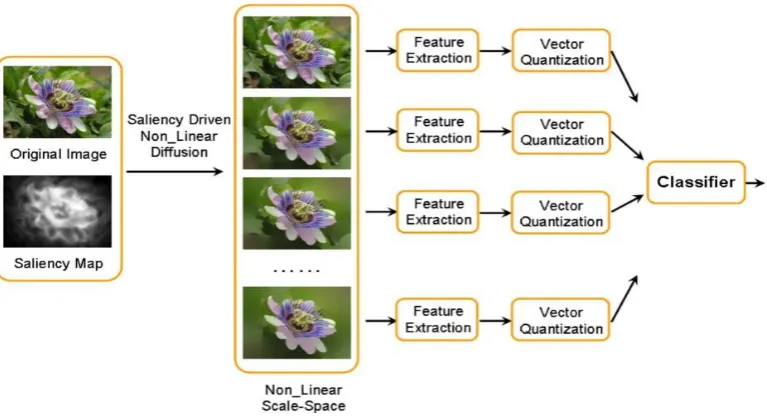
4. Multi-Scale Image Representation and Classification
Figure 7. The framework of the multi-scale representation for image classification.
We propose to classify images using the saliency driven multi-scale image representation. Images whose
foregrounds are clearer than their backgrounds are more likely to be correctly classified at a large scale, and
images whose backgrounds are clearer are more likely to be correctly classified at a small scale. So, information
from different scales can be fused to acquire more accurate image classification results. Our image classification
framework is shown in Figure 7. Each image is represented by its multi-scale images. Then, for each scale t,
scale invariant feature transform (SIFT) features, which are widely used to represent image regions, are extracted,
and the bag-of-words model is used to generate a word frequency histogram
h
t. The dissimilarity betweenimages 1 and 2 at scale t is represented by the
2 distanced h h
( ,
1t 2t)
between histogramsh
1t andh
2t. Thedistances
{ ( ,
d h h
1t 2t)}
t T between images 1 and 2 obtained at different scales are combined to yield the final [image:12.595.107.491.261.471.2]1 2 1 2
( ,
)
( ,
)
t t t t T t t Tw d h h
d h h
w
(12)where
w
t is a weight for scale t, and T is a chosen set of scales. Weighted averaging, which is a general way forinformation fusion, is used to fuse information from different scales. By selecting appropriate weights, the
distances between samples in the same class can be reduced and the distances between samples in different
classes can be enlarged. Then, more accurate classification results can be obtained. This weighted averaging has
been widely used in many applications. For example, Wu [45] applied the weighted averaging to product
recommendation and it was shown that the weighted averaging improves the prediction accuracy.
In this paper, we empirically use three representative scales:
T
{ ,
T T T
0 m,
M}
, whereT
M is themaximum scale at which the diffusion process converges,
T
0
0
, andT
m is a mid-scale which is set toint(
T
M/ 3)
. The three scales are combined using (12). The reasons for selecting these three scales are asfollows:
When the scale is larger than
T
M, there is almost no change in the diffused image. At scaleT
M,foreground/background segmentation is completed.
The inclusion of the original image corresponding to scale
T
0 in T can provide a correction if theforeground is incorrectly filtered out and using the image at scale
T
M alone is not sufficient to obtaina correct classification result.
The mid-scale
T
m is a compromise between smoothing the background and preserving the foreground.Although there are no clear cut criteria to pick the mid-scale
T
m, the experiments show that the use ofm
T
improves the classification.The weights
w
0,m T
w
, andM T
w
are determined empirically using the training samples. The values of theweights
w
0,m T
w
, andM T
w
reflect the situations of the correction segmentation of the foreground in thetraining samples. If the weight for one scale is set to 0, three-scale fusion degenerates to two-scale fusion. In
particular, fusion of scale 0 and scale TM produces a combination of the original image and the foreground image,
which is equivalent to using the original image with more weight given to the foreground.
scales, is transformed to a kernel which is used by an SVM for classification. We use the extended Gaussian
kernels:
1 2
1 2
1
,
exp
,
K h h
d h h
A
(13)where A is a scaling parameter that can be determined by cross-validation. An SVM classifier is trained using the
kernel matrix of the training images.
The proposed saliency driven multi-scale fusion uses the background information in a new way. At a large
scale, the background is filtered out and the foreground is preserved. At a small scale, both the background and
the foreground regions are preserved. When the background is a context for the foreground, the images from the
same category are more similar at a small scale than at a large scale. When the background is noise, the images
are more similar at a large scale. Through this multi-scale representation, background information can be utilized.
We define the distance between two images as a weighted average of the distances in the different used scales as
shown in (12), instead of the minimum of their distances at all scales. The use of a weighted average reduces the
classification error in cases in which the foreground is incorrectly filtered.
Our saliency driven nonlinear multi-scale representation has several advantages: First, the nonlinear
diffusion-based multi-scale space can preserve or enhance semantically important image structures at large
scales. In particular, the saliency driven nonlinear diffusion can divide the foreground from the background at
large scales, with only a little loss of the foreground information. Second, our method can deal with the
background information no matter whether it is a context or noise, and then can be adapted to backgrounds
which change over time. Third, our method can partly handle cases in which the saliency map is incorrect, by
including the original image at scale 0 in the set of scaled images used for classification. Finally, this saliency
driven multi-scale representation can be easily combined with any existing image classification algorithms (e.g.
bag-of-words).
The baseline of our work is nonlinear diffusion filtering [30]. We extend the baseline in the following ways:
The saliency detection technique is combined with nonlinear diffusion filtering.
Multi-scale fusion is used to combine the information from the saliency driven nonlinear diffusion
filtering.
We apply the proposed filtering and fusion method to image classification. To our knowledge, there is
no other work which applies nonlinear diffusion filtering to image classification.
We tested our image classification algorithm based on the proposed saliency driven nonlinear diffusion
filtering and multi-scale fusion on four public datasets: the PASCAL VOC 2005 Test2 dataset [4], the 102
Oxford Flowers dataset [18], the 17 Oxford Flowers dataset [19], and a people dataset. For all the datasets, the
values of the parameters C and m in (8) were set to 1 and 100, respectively.
5.1. PASCAL VOC 2005
The PASCAL VOC 2005 dataset [4] for image classification has an easy test set (test1) and a difficult test
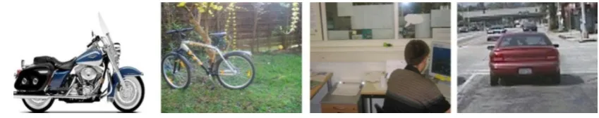
set (test2). We focused on the difficult set because the performance on the easy set is saturated. The set test2 has
four categories: motorbike, bicycle, car, and persons, and contains 1543 images. Figure 8 shows some example
images from the set. The best score in the competition of test2 was achieved in [4] by using the bag-of-words
[image:15.595.81.506.310.394.2]model.
Figure 8. Example images from the test2 set in the PASCAL VOC 2005 dataset: one image per category.
For each scale in the set
{ ,
T T T
0 m,
M}
described in Section 4, we followed the experimental setup in [4]:the Harris-Laplace detector and the SIFT descriptor were used and 1000 visual words were extracted using
k-means from the training set. The weights
w
0,m T
w
, andM T
w
were set to 1, 2, and 1, respectively.The main point in which our method differs from [4] is that we used the
2 distance in Equation (12)which fuses the
2 histogram distances in the three scales, to estimate the distance between any two images.In [4], the
2 histogram distance did not make use of images at different scales. Libsvm [2] was used and theparameter of SVM was determined using the two-fold cross-validation on the training set.
Table 1 compares the classification results of different methods applied to test2 in the PASCAL 2005 set.
Compared with all the other reported results, our method obtains the best performance not only for average rates
over all the categories, but also for the bike and person categories. The performance of our method for the car
category is very close to the best. Our method obtains much better results than [4] for three categories: bike,
person, and car, but a worse result for the motorbike category. This is because there are many motorbike images
which have very little background (for example the left image in Figure 8). Our method gains an advantage by
categories have considerable background regions which our method can take advantage of.
Table 1. Correct classification rates (at equal error rates) on the PASCAL challenge 2005 Test Set 2
Motor Bike Person Car Average
Winner(2) [4]
79.8% 72.8% 71.9% 72.0% 74.1%
Winner(EMD) [33] 79.7% 68.1% 75.3% 74.1% 74.3%
PDK [15] 76.9% 70.1% 72.5% 78.4% 74.5%
Xie [31] 79.1% 75.4% 73.9% 78.2% 76.7%
Proposed method 77.50% 75.56% 76.08% 78.24% 76.85%
5.2. 102 Oxford Flowers
The 102 Oxford Flowers dataset [18] contains 8189 images from 102 flower categories with 40-250 images
per category. For each category, 10 images were used for training, 10 for validation, and the rest for testing, as
the same as in [18]. At each scale, we used the same experimental setup as in [22, 31]. For each image, two
sampling methods, the Harris-Laplace point sampling and dense sampling, were used to generate local patches
where each patch corresponds to a point of interest. Then, each image patch was further represented by the SIFT
and the four color-SIFT descriptors [24]: OpponentSIFT, rgSIFT, C-SIFT, and RGB-SIFT. These color-SIFT
descriptors which have specific invariance properties were used to improve classification performance [24]. For
each type of descriptor, the training images were clustered using k-means to generate a vocabulary of 4000
words. Soft coding was used to generate feature vectors of images. Three different image division modes were
used to represent each image: the whole image without subdivision (1x1), 4 image parts obtained by dividing the
image into 4 quarters (2x2) and 3 image parts obtained by dividing the image into three horizontal bars (1x3).
The
2 distance was used to calculate histogram distances. The weightsw
0,m T
w
, andM T
w
were set to 1, 2,and 0, respectively. The distances at the three scales were combined using (12). An SVM classifier was trained
using the training images. The parameters were estimated on the validation set and further used on the test set.
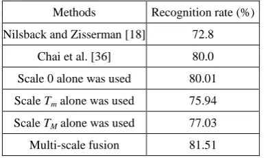
Table 2. The recognition rates of different methods on the 102 Oxford flower dataset
Methods Recognition rate (%)
Nilsback and Zisserman [18] 72.8
Chai et al. [36] 80.0
Scale 0 alone was used 80.01
Scale Tm alone was used 75.94
Scale TM alone was used 77.03 Multi-scale fusion 81.51
As stated in [36], among all recent approaches evaluated on the 102 Oxford flowers dataset, the most
[image:16.595.202.395.605.720.2]36] along with our multi-scale fusion method. It is seen that our multi-scale method yields more accurate results
than the single scale methods in [18] and [36]. Table 3 compares the results of multi-scale fusion with the results
for the individual scales
T
0,T
m, andT
M. The recognition rate for multi-scale fusion is higher than for thesingle scales
T
0,T
m, andT
M.Table 3. Comparison between the single scale methods and the multi-scale fusion method onthe 102 Oxford flower dataset
From scale 0 to multi-scale
From scale Tm to multi-scale
From scale TM to multi-scale Number of categories whose
accuracies increase by more than 5% 12 40 21 Number of categories whose
accuracies increase 44 63 45
Number of categories whose
accuracies decrease 27 11 18
Number of categories whose
accuracies decrease by more than 5% 5 2 5
To show how the fusion of multi-scales works, we give example images that are classified differently by
single scale methods and by the multi-scale fusion.
[image:17.595.127.462.187.298.2]Original image Scale Tm Scale TM Saliency
Figure 9. Example images that were correctly classified at scales Tmand TM, and by multi-scale fusion, but incorrectly classified at scale 0.
Figure 9 shows two images that were correctly classified by scales
T
m,T
M and by multi-scale fusion, butincorrectly classified at scale 0. Both the two original images contain large areas of background. In their saliency
maps, the foreground regions were correctly detected. Our saliency driven nonlinear diffusion preserved their
foreground regions and largely smoothed the background regions. Therefore, at scales
T
m andT
M in whichthe backgrounds were filtered out, the images were correctly classified. This produces a correct classification by
[image:17.595.129.467.363.572.2]Figure 10 shows two example images that were correctly classified at scale 0 and by multi-scale fusion, but
incorrectly classified at scales
T
m andT
M. The saliency maps incorrectly identified the background andforeground regions. As a result, the saliency driven diffusion smoothed several flowers into a single connected
region, and erased the appearances and shapes of the flowers. As a result, the information from scales
T
m andM
T
is unreliable for these images. However, because the original image is included in the fusion, correct finalclassification results are obtained.
[image:18.595.100.495.232.438.2]Original image Scale Tm Scale TM Saliency
Figure 10. Example images that were correctly classified at scale 0 and by multi-scale fusion, but incorrectly classified at scales Tm and TM.
[image:18.595.154.443.483.682.2]Original image Scale Tm Scale TM Saliency
Figure 11. Images that were correctly classified at scale 0, but incorrectly classified at scales Tmand TM, and by multi-scale fusion.
Figure 11 shows two example images that were correctly classified at scale 0, but incorrectly classified at
scales
T
m andT
M, and by multi-scale fusion. The background region was incorrectly classed as salient and theflowers, and erased their appearances and shapes. Although the classification result at scale 0 is correct, the large
biases at scales
T
m andT
M make classification based on multi-scale fusion incorrect. These examplesdemonstrate that, although the original image is included in the multi-scale fusion, our method still occasionally
suffers from the incorrect detection of saliency while overall increasing the classification performance.
5.3. 17 Oxford Flowers
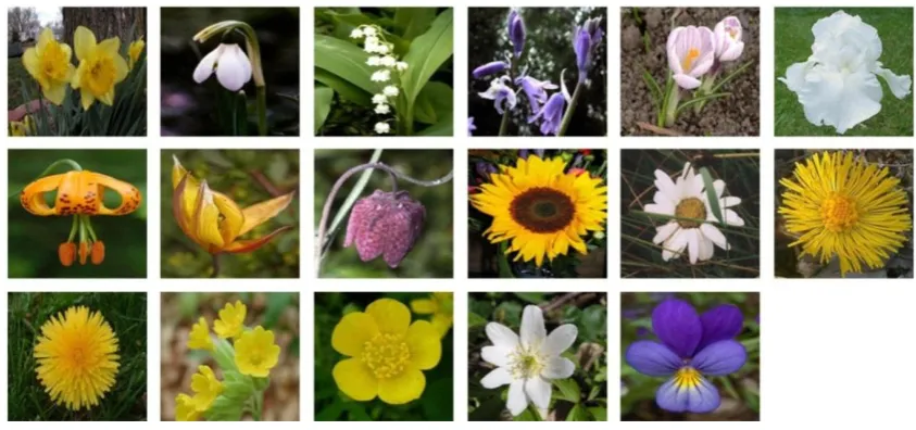
The 17 Oxford Flowers dataset [19] contains images from 17 flower categories with 80 images per category.
Figure 12 shows some example images in the dataset. For each flower category, 40 images were used for
training, 20 for validation, and 20 for testing. For comparison, we divided the dataset into the same training,
validation and test sets used in [19]. In each scale, we used the same experimental setup as in [31]. The
experiments include:
two types of sampling -- the Harris-Laplace sampling and the dense sampling
five types of descriptor -- the SIFT and four types of the color-SIFT descriptors
three types of image division -- 1x1, 2x2, and 1x3.
In total, 30 (2x5x3) channels of features were used and combined by averaging the histogram distances of each
channel. For each type of descriptor, a kernel codebook of 4000 code words was constructed using k-means. The
experimental arrangements are the same at each of the three scales, to avoid bias. The weights
w
0,m T
w
, andM T
[image:19.595.86.508.497.695.2]w
were set to 1, 2, and 1, respectively. Then, three scales were combined using (12).Figure 12. Example images from the Oxford Flowers dataset, one per category.
Figure 13 shows some examples of filtered images obtained using our saliency driven nonlinear diffusion. It
background.
Figure 13. Examples of filtered images in the Oxford 17 flowers dataset: The first row shows the original images; The second row
[image:20.595.202.393.318.514.2]shows the saliency masks; The third row shows the filtered images at scale TM. The columns correspond to distinct categories.
Table 4. The recognition rates of different methods on the 17 Oxford flower dataset
Methods Recognition rate (%)
Nilsback and Zisserman [19] 71.76% ±1.76
Varma and Ray [26] 82.55±0.34
Nilsback and Zisserman [18] 88.33±0.3
Xie [31] 89.02±0.60
Khan [13] 89
Gehler and Nowozin [6] 85.5±1.2
Chai et al. [36] 90.40±2.3
Scale 0 87.45±1.13
Scale Tm 87.69±1.61 Scale TM 88.21±1.19 Multi-scale fusion 91.39±0.53
Table 4 summarizes the published recognition accuracies for several methods from the literature, along with
the accuracy of our multi-scale fusion method. The average accuracy of classification and the variance were
reported. The results of our method are more accurate than other reported results. Multi-scale fusion obtains
more accurate results than those obtained using the individual scales
T
0,T
m, orT
M. This indicates that thethree scales include complementary information, and their fusion can improve the classification results.
5.4. The people dataset
This dataset consists of 460 people images available at http://www.emt.tugraz.at/~pinz/data/ GRAZ_01/,
100 images from video streams with time-varying backgrounds, and 600 non-people images. It includes
pedestrians, diverse background conditions/clutter, and occlusions. Figure 14 shows some example images in the
image with a group of people with occlusion, (d) is an image with diverse background conditions, and (c) is an
image with background clutter.
[image:21.595.90.508.114.198.2](a) (b) (c) (d) (e)
Figure 14. Example images from the people dataset: (a) Single pedestrian; (b) Two people with occlusion; (c) A group of people
[image:21.595.87.510.251.413.2]with occlusions; (d) Diverse background conditions; (e) Background clutter.
Figure 15. Examples ofthe results for the still images with static backgrounds in the people dataset: The first row shows the
original images; The second row shows the saliency masks; The third row shows the filtered images at the scale TM.
Figure 16. The results of saliency detection and nonlinear diffusion for the images from three videos with dynamic background variations: The first row shows the original images; The second row shows the saliency masks; The third row shows the filtered
images at the scale TM.
Half of the images in the dataset were used for training and the other half of the images were used for
testing. For each scale of each image, the Harris-Laplace sampling and the dense sampling are used respectively,
[image:21.595.89.510.468.628.2]sampling strategy, the weights
w
0,m T
w
, andM T
w
were set to 1, 1, and 4, respectively. For the Harris-Laplacesampling strategy, the weights were set to 1, 2, and 4, respectively. Figures 15 and 16 show some examples of
the results of saliency detection and nonlinear diffusion for still images and images from videos, respectively. It
is seen that, overall the detected salient regions correspond to the foreground and in the final filtered image much
of the background is filtered out. Table 5 shows the results of image classification on this dataset. It is seen that
large scales yield more accurate results than using the original images, and the fusion of multi-scales yields more
accurate results than using a single scale alone. Our saliency driven nonlinear diffusion and multi-scale fusion
[image:22.595.208.389.277.380.2]significantly improve the results.
Table 5. The recognition rates of different scales and fusions for multi-scales on the people dataset
Methods
Recognition rate (%) Dense
sampling
Harrislaplace sampling Scale 0 89.03 83.72
Scale Tm 89.12 85.89
Scale TM 92.71 86.68 Multi-scale fusion 94.03 87.42
5.5. Processing time
The processing time was measured on an Intel Core i7 3770(3.4GHz/L3) computer. The runtime of
nonlinear diffusion filtering for each image in all the datasets is less than 2 seconds. The training time for each
dataset used is less than 300 seconds. The test time for each image is less than 0.01 seconds.
5.6. Discussion
Our fusion method with three scales
T
{ ,
T T T
0 m,
M}
achieves the best classification accuracies amongall those reported for the PASCAL 2005 dataset, the Oxford 102 flowers dataset, the Oxford 17 flowers dataset,
and the people dataset.
The experiments on the Oxford 17 flowers dataset show that the classification accuracies obtained by our
method for filtered images alone are higher than those for the initial unfiltered images. On the Oxford 102
flowers dataset, the accuracies for filtered images are slightly lower than the accuracies for the initial images.
This effect is caused by saliency detection errors which depend on the saliency detection algorithm. The error
metrics for saliency detection include precision, recall and the F1 measure. The datasets do not include ground
truth saliencies, so we have estimated the errors in saliency detection by our own observations. When the
detected saliency masks are correct, semantically important foregrounds are effectively preserved, while
semantically important foregrounds are partially or totally smoothed, and cluttered backgrounds are partially or
totally preserved. The results of saliency detection on the Oxford 17 flowers dataset, which is comparatively
simple, are more accurate than the results of saliency detection on the Oxford 102 flowers dataset. Then, filtering
by itself improves classification accuracy for the Oxford 17 flowers dataset, and reduces classification accuracy
for the Oxford 102 flowers dataset. But, the fusion of the results for the original images and the results for
filtered images yields more accurate results than using the original images or the filtered images alone. So,
multi-scale fusion improves the final classification accuracy.
6. Conclusion
In this paper, we have proposed saliency driven multi-scale nonlinear diffusion filtering, by modifying the
mathematical equations for nonlinear diffusion filtering, and determining the diffusion parameters using the
saliency detection results. We have further applied this new method to image classification. The saliency driven
nonlinear multi-scale space preserves and even enhances important image local structures, such as lines and
edges, at large scales. Multi-scale information has been fused using a weighted function of the distances between
images at different scales. The saliency driven multi-scale representation can include information about the
background in order to improve image classification. Experiments have been conducted on widely used datasets,
namely the PASCAL 2005 dataset, the Oxford 102 flowers dataset, and the Oxford 17 flowers dataset. The
results have demonstrated that saliency driven multi-scale information fusion improves the accuracy of image
classification.
References
[1] Y. Boureau, F. Bach, Y. LeCun, and J. Ponce, “Learning Midlevel Features for Recognition,” in Proc. of IEEE Conference on
Computer Vision and Pattern Recognition, pp. 2559-2566, June 2010.
[2] C.-C. Chang and C.-J. Lin, “LIBSVM: a Library for Support Vector Machines,” http://www.csie.ntu.edu.tw/»cjlin/libsvm/,
2001.
[3] F. D’Almeida, “Nonlinear Diffusion Toolbox,” MATLAB Central, July 2003. http://www.mathworks.cn/matlabcentral/
fileexchange/3710-nonlinear-diffusion-toolbox
[4] M. Everingham, A. Zisserman, C. K. I. Williams, L. van Gool, M. Allan, C. M. Bishop, O. Chapelle, N. Dalal, T. Deselaers, G.
Dorko, S. Duffner, J. Eichhorn, J. D. R. Farquhar, M. Fritz, C. Garcia, T. Griffiths, F. Jurie, D. Keysers, M. Koskela, J.
Laaksonen, D. Larlus, B. Leibe, H. Meng, H. Ney, B. Schiele, C. Schmid, E. Seemann, J. Shawe-Taylor, A. Storkey, S.
Szedmak, B. Triggs, I. Ulusoy, V. Viitaniemi, and J. Zhang, “The 2005 PASCAL Visual Object Classes Challenge,” in Proc.
of the first PASCAL Challenges Workshop, Lecture Notes in Artificial Intelligence, no. 3944, pp. 117-176, Southampton, UK,
2006
[5] C. Galleguillos, A. Rabinovich, and S. Belongie, “Object Categorization Using Co-occurrence, Location and Appearance,” in
[6] P. Gehler and S. Nowozin, “On Feature Combination for Multiclass Object Classification,” in Proc. of IEEE International
Conference on Computer Vision, pp. 221-228, 2009.
[7] S. Goferman, L. Zelnik-Manor, and A. Tal, “Context-Aware Saliency Detection,” in Proc. of IEEE Conference on Computer
Vision and Pattern Recognition, pp. 2376-2383, 2010.
[8] K. Grauman and T. Darrell, “The Pyramid Match Kernel: Efficient Learning with Sets of Features,” Journal of Machine
Learning Research, vol. 8, no. 4, pp. 725-760, April 2007.
[9] J. Harel, C. Koch, and P. Perona, “Graph-Based Visual Saliency,” in Proc. of Annual Conference on Neural Information
Processing Systems, pp. 545-552, 2007.
[10]G. Heitz and D. Koller, “Learning Spatial Context: Using Stuff to Find Things,” in Proc. of European Conference on
Computer Vision, pp. 30-43, 2008.
[11]X. Hou and L. Zhang, “Saliency Detection: a Spectral Residual Approach,” in Proc. of IEEE Conference on Computer Vision
and Pattern Recognition, pp. 1-8, 2007.
[12]L. Itti, C. Koch, and E. Niebur, “A Model of Saliency-Based Visual Attention for Rapid Scene Analysis,” IEEE Trans. on
Pattern Analysis and Machine Intelligence, vol. 20, no. 11, pp. 1254-1259, Nov. 1998.
[13]S. Khan, J. van de Weijer, and M. Vanrell, “Top-Down Color Attention for Object Recognition,” in Proc. of IEEE
International Conference on Computer Vision, pp. 979-986, 2009.
[14]S. Lazebnik, C. Schmid, and J. Ponce, “Beyond Bags of Features: Spatial Pyramid Matching for Recognizing Natural Scene
Categories,” in Proc. of IEEE Conference on Computer Vision and Pattern Recognition, vol. 2, pp. 2169-2178, 2006.
[15]H. Ling and S. Soatto, “Proximity Distribution Kernels for Geometric Context in Category Recognition,” in Proc. of IEEE
International Conference on Computer Vision, pp. 1-8, Oct. 2007.
[16]T. Liu, Z. Yuan, J. Sun, J. Wang, N. Zheng, X. Tang, and H.-Y. Shum, “Learning to Detect a Salient Object,” IEEE Trans. on
Pattern Analysis and Machine Intelligence, vol. 33, no. 2, pp. 35 -367, Feb. 2011.
[17]L. Marchesotti, C. Cifarelli, and G. Csurka, “A Framework for Visual Saliency Detection with Applications to Image Thumb
Nailing,” in Proc. of IEEE International Conference on Computer Vision, pp. 2232-2239, 2009.
[18]M.E. Nilsback and A. Zisserman, “Automated Flower Classification over a Large Number of Classes,” in Proc. of Indian
Conference on Computer Vision, Graphics and Image Processing, pp. 722-729, Feb. 2008.
[19]M.-E. Nilsback and A. Zisserman, “A Visual Vocabulary for Flower Classification,” in Proc. of IEEE Conference on Computer
Vision and Pattern Recognition, vol. 2, pp. 1447-1454, 2006.
[20]P. Perona and J. Malik, “Scale-Space and Edge Detection Using Anisotropic Diffusion,” IEEE Trans. on Pattern Analysis and
Machine Intelligence, vol. 12, no. 7, pp. 629-639, July 1990.
[21]J. Shotton, J. Winn, C. Rother, and A. Criminisi, “Textonboost: Joint Appearance, Shape and Context Modeling for
Multi-Class Object Recognition and Segmentation,” in Proc. of European Conference on Computer Vision, pp. 1-15, 2006.
[22]M. Tahir, J. Kittler, K. Mikolajczyk, F. Yan, K.E.A. van de Sande, and T. Gevers, “Visual Category Recognition Using
Spectral Regression and Kernel Discriminant Analysis,” in Proc. of IEEE International Workshop on Subspace, Kyoto Japan,
pp. 178-185, Jan. 2009.
[23]R. Valenti, N. Sebe, and T. Gevers, “Image Saliency by Isocentric Curvedness and Color,” in Proc. of IEEE International
Conference on Computer Vision, pp. 2185-2192, 2010.
[24]K.E.A. van de Sande, T. Gevers, and C.G.M. Snoek, “Evaluation of Color Descriptors for Object and Scene Recognition,”
IEEE Trans. on Pattern Analysis and Machine Intelligence, vol. 32, no. 9, pp. 1582-1596, Sep. 2010.
[25]J.C. van Gemert, C.J. Veenman, A.W.M. Smeulders, and J.M. Geusebroek, “Visual Word Ambiguity,” IEEE Trans. on
[26]M. Varma and D. Ray, “Learning the Discriminative Power Invariance Trade-Off,” in Proc. of IEEE International Conference
on Computer Vision, pp. 1-8, Oct. 2007.
[27]D.Walther and C. Koch, “Modeling Attention to Salient Protoobjects,” Neural Networks, vol. 19, no. 9, pp. 1395-1407, 2006.
[28]J. Wang, J. Yang, K. Yu, F. Lv, T. Huang, and Y. Gong, “Locality-Constrained Linear Coding for Image Classification,” in
Proc. of IEEE Conference on Computer Vision and Pattern Recognition, pp. 3360-3367, June 2010.
[29]J. Weickert, “A Review of Nonlinear Diffusion Filtering,” Scale-Space Theory in Computer Vision, Lecture Notes in
Computer Science, vol. 1252, pp. 1-28, 1997.
[30]J. Weickert, B. Romeny, and M.A. Viergever, “Efficient and Reliable Schemes for Nonlinear Diffusion Filtering,” IEEE Trans.
on Image Processing, vol. 7, no. 3, pp. 398-410, 1998.
[31]N. Xie, H. Ling, W. Hu, and X. Zhang, “Use Bin-Ratio Information for Category and Scene Classification,” in Proc. of IEEE
Conference on Computer Vision and Pattern Recognition, pp. 2313-2319, June 2010.
[32]J. Yang, K. Yu, and T. Huang, “Supervised Translation Invariant Sparse Coding,” in Proc. of IEEE Conference on Computer
Vision and Pattern Recognition, pp. 3517-3524, 2010.
[33]J. Zhang, M. Marszalek, S. Lazebnik, and C. Schmid, “Local Features and Kernels for Classification of Texture and Object
Categories: a Comprehensive Study,” International Journal of Computer Vision, vol. 73, no. 2, pp. 213-238, June 2007.
[34]M. M. Cheng, G. X. Zhang, N. J. Mitra, X. L. Huang, and S. M. Hu, “Global Contrast Based Salient Region Detection,” in
Proc. of IEEE Conference on Computer Vision and Pattern Recognition, pp. 409-416, 2011.
[35]F. Li, G. Lebanon, and C. Sminchisescu, “Chebyshev Approximations to the Histogram χ2 Kernel,” in Proc. of IEEE
Conference on Computer Vision and Pattern Recognition, pp. 2424-2431, 2012.
[36]Y. Chai, V. Lempitsky, and A. Zisserman, “BiCoS: A Bi-Level Co-segmentation Method for Image Classification,” in Proc. of
IEEE International Conference on Computer Vision, pp. 2579-2586, Nov. 2011.
[37]T. Judd, K.A. Ehinger, F. Durand, and A. Torralba, “Learning to Predict where Humans Look,” in Proc. of IEEE International
Conference on Computer Vision, pp. 2106-2113, 2009.
[38]H. Jiang, J. Wang, Z. Yuan, Y. Wu, N. Zheng, and S. Li, “Salient Object Detection: a Discriminative Regional Feature
Integration Approach,” in Proc. of IEEE Conference on Computer Vision and Pattern Recognition, 2013.
[39]R. Achanta, S. Hemami, F. Estrada, and S. Susstrunk, “Frequency-Tuned Salient Region Detection,” in Proc. of IEEE
Conference on Computer Vision and Pattern Recognition, pp. 1597-1604, 2009.
[40]X.-H. Shen and Y. Wu, “A Unified Approach to Salient Object Detection via Low Rank Matrix Recovery,” in Proc. of IEEE
Conference on Computer Vision and Pattern Recognition, pp. 853-860, 2012.
[41]M.T. Mahmood and T.-S. Choi, “Nonlinear Approach for Enhancement of Image Focus Volume in Shape from Focus,” IEEE
Trans. on Image Processing, vol. 21, no. 5, pp. 2866-2873, 2012.
[42]M.R. Hajiaboli, M.O. Ahmad, and C. Wang, “An Edge-Adapting Laplacian Kernel for Nonlinear Diffusion Filters,” IEEE
Trans. on Image Processing, vol. 21, no. 4, pp. 1561-1572, 2012.
[43]P. Rodrigues and R. Bernardes, “3-D Adaptive Nonlinear Complex-Diffusion Despeckling Filter,” IEEE Trans. on Medical
Imaging, vol. 31, no. 12, pp. 2205-2212, 2012.
[44]B. Abdollahi, A. El-Baz, and A.A. Amini, “A Multi-Scale Non-linear Vessel Enhancement Technique,” in Proc. of Annual
International Conference of the IEEE Engineering in Medicine and Biology Society, pp. 3925-3929, 2011.
Acknowledgments
This work is partly supported by the 973 basic research program of China (Grant No. 2014CB349303), the
National 863 High-Tech R&D Program of China (Grant No. 2012AA012504), the Natural Science Foundation
of Beijing (Grant No. 4121003), and The Project Supported by Guangdong Natural Science Foundation (Grant
No. S2012020011081).
Weiming Hu received the Ph.D. degree from the department of computer science and engineering, Zhejiang University in 1998. From April 1998 to March 2000, he was a postdoctoral research fellow with the Institute of Computer Science and Technology, Peking University. Now he is a professor in the Institute of Automation, Chinese Academy of Sciences. His research interests are in visual motion analysis, recognition of web objectionable information, and network intrusion detection.
Ruiguang Hu received both the Bachelor and Master degrees from the College of Optoelectronic Engineering at Chongqing University in 2006 and 2009. Now he is a PhD candidate working in the National Laboratory of Pattern Recognition, Institute of Automation, Chinese Academy of Sciences, Beijing, China. His research interests include computer vision, machine learning, image classification, object recognition, saliency detection, information fusion, and Internet content security.
Nianhua Xie received the B.E. degree in automation engineering from the Beijing Institute of Technology, Beijing, China, in 2005. In 2011, he received the Ph.D degree in the Institute of Automation, Chinese Academy of Sciences, Beijing, China. In July 2011, he joined the Beijing Sogou Technology Development Company as a business Ad researcher. His research interests include image processing, computer vision and machine learning.
Haibin Ling received the BS degree and the MS degree from Peking University, China, in 1997 and 2000, respectively, and the PhD degree from the University of Maryland, College Park, in 2006. From 2006 to 2007, he worked as a postdoctoral scientist at the University of California Los Angeles. After that, he joined Siemens Corporate Research as a research scientist. Since Fall 2008, he has been an assistant professor at Temple University. His research interests include computer vision, medical image analysis, human computer interaction, and machine learning.