Water waves and Integrability

arXiv:0707.1839v1 [nlin.SI] 12 Jul 2007

Water waves and integrability

Rossen I. Ivanov∗1

School of Mathematics, Trinity College, Dublin 2, Ireland

∗_{e-mail: [email protected]}

Abstract

The Euler’s equations describe the motion of inviscid fluid. In the case of shallow water, when a perturbative asymtotic expansion of the Euler’s equations is taken (to a certain order of smallness of the scale parameters), relations to certain integrable equations emerge. Some recent results concerning the use of integrable equation in modeling the motion of shallow water waves are reviewed in this contribution.

Key Words: Euler’s equations, Integrability, Camassa-Holm equa-tion, Degasperis-Procesi equaequa-tion, Korteweg-de Vries equation.

1

Governing equations for the inviscid fluid

mo-tion

The motion of inviscid fluid with a constant density ρ is described by the Euler’s equations:

∂v

∂t + (v· ∇)v = −

1

ρ∇P +g, (1)

∇ ·v = 0, (2)

wherev(x, y, z, t) is the velocity of the fluid at the point (x, y, z) at the time

t,P is the pressure in the fluid,g= (0,0,₋g) is the constant Earth’s gravity acceleration.

Consider now a motion of a shallow water over a flat bottom, which is located at z = 0. We assume that the motion is in the x-direction, and that the physical variables do not depend on y. Let h be the mean level of

the water and let η(x, t) describes the shape of the water surface, i.e. the deviation from the average level. The pressure is

P =PA+ρg(h−z) +p(x, z, t), (3)

wherePAis the constant atmospheric pressure, andpis a pressure variable,

measuring the deviation from the hydrostatic pressure distribution. On the surface z = h+η, P = PA and therefore p = ηρg. Taking v ≡ (u,0, w)

we can write the kinematic condition on the surface as [e.g. see (Johnson 1997)]

w= ∂η

∂t +u

∂η

∂x on z=h+η. (4)

Finally, there is no horizontal velocity at the bottom, thus

w= 0 on z= 0. (5)

The equations (1) – (5) give the system

ut+uux+wuz =−

1

ρpx,

wt+uwx+wwz =−

1

ρpz, ux+wz = 0,

w=ηt+uηx, p=ηρg, on z=h+η,

w= 0 on z= 0.

(6)

Let us introduce now dimensionless parameters ε = a/h and δ = h/λ, whereais the typical amplitude of the wave andλis the typical wavelength of the wave. Now we can introduce dimensionless quantities, according to the magnitude of the physical quantities, see (Johnson 1997, 2002) for details:

x_→λx, z_→zh, t_→ √λ

ght, η→aη,

u_→εpghu, w_→εδpghw, p_→ερgh.

ut+ε(uux+wuz) =−px,

δ2(wt+ε(uwx+wwz)) =−pz,

ux+wz= 0,

w=ηt+εuηx, p=η, on z= 1 +εη,

w= 0 on z= 0.

(7)

For the right-running waves one can introduce the so-called far field quantities, see (Johnson 1997, 2002, 2003a)

ζ =√ε(x₋t), τ =ε3/2t, w=√εW, (8)

and the system (7) acquires the form

εuτ −uζ+ε(uuζ+W uz) =−pζ, (9)

εδ2(εWτ−Wζ+ε(uWζ+W Wz)) =−pz, (10)

uζ+Wz= 0, (11)

W =εητ−ηζ+εuηζ, p=η, on z= 1 +εη, (12)

W = 0 on z= 0. (13)

2

Asymptotic expansion of the variables

Following the idea of Johnson (2002), we can express the variablesu,W,p

as double-asymptotic expansion (inεand δ) with terms, depending only on

η(x, t) and explicitly onz. As a result, a single nonlinear equation forηwill be obtained, and thus all variables will be expressed through the solution of this equation.

From (10) it is evident that pz =O(εδ2), and thus in the leading order

pdoes not depend on z, i.e.

p=η. (14)

Substitution of (14) into (9) and (11) gives for the leading orders

u=η, W =₋zηζ. (15)

Consider the next terms (first corrections) in the expansion ofuandW, denoted by E(u), E(W), which possibly contain terms of orders ε and δ2. Writing u=η+E(u), W =₋zηζ+E(W), from (9) it follows

and from (11), (13) and (16),

E(W) = ₋

Z

Eζ(u)dz=−εz(ητ +ηηζ),

W = ₋z(ηζ+εητ +εηηζ). (17)

Now the substitution of (17) into (12) gives the leading order equation forη:

ητ =−

3

2ηηζ+O(ε, δ

2_{). (18)}

From (18) and (16) we obtain E(u) = ₋εη2_{/4, i.e. no δ}2 _{term is present} and finally, using (17) and (18),

u=η₋ε

4η

2_{, W =−zη}

ζ−

ε

2ηηζ

. (19)

Using (15) in (10) we have pz = −εδ2zηζζ. This can be integrated due

to (12) and thus we obtain the next order approximation forp:

p=η₋εδ21−z

2

2 ηζζ. (20)

We accomplished the first step, i.e. starting from the leading order (14), (15), we obtained the first corrections (19), (20) and an equation forη, (18). The next step can be performed in a similar fashion and it gives

u = η₋ ε

4η 2₊ε2

8 η

3_+εδ21 3−

z2 2

ηζζ, (21)

W = ₋zηζ−

ε

2ηηζ+ 3ε2

8 η 2_η

ζ

+εδ2₋ z

3+

z3 6

ηζζζ, (22)

p = η₋εδ21−z

2

2 ηζζ+ε 2_δ2_(ηη

ζζ+ (1−z2)ηζ2), (23)

whereη(x, t) satisfies the equation

ητ =−

3 2ηηζ+

3 8εη 2_η ζ− 1 6δ 2_η

ζζζ+O(ε2, δ4, εδ2). (24)

We observe, that at the end of each step the equation for η(x, t) contains terms of smaller order than those, which appear in the expressions foruand

ητ =−

3 2ηηζ+

3 8εη 2_η ζ− 3 16ε

2_η3_η

ζ−

1 6δ

2_η

ζζζ

−₂₄1 εδ2(23ηζηζζ+ 10ηηζζζ) +O(ε3, δ6, ε2δ2, εδ4). (25)

Now, we can invert (21) by specifyingu at a specific depth,z0 (0_≤z0≤1): defining ˆu=u(ζ, τ, z0), we obtain

η= ˆu+ε

4uˆ 2

−εδ2λuˆζζ+O(ε3, δ6, εδ4, ε2δ2), (26)

where

λ_≡ 1

3 −

z₀2

2 , −

1

6 ≤λ≤ 1

3. (27)

Note that in (26) there is no term of orderε2. The substitution of (26) in (25) yields:

ˆ

uτ =−

3 2uˆuˆζ−

1 6δ

2_uˆ

ζζζ−

1 2εδ

2h29 12 + 6λ

ˆ

uζuˆζζ +

5 6uˆuˆζζζ

i

+O(ε3, δ6, ε2δ2, εδ4). (28)

Next, we go back to the original variables, introducingT _≡√εt,X_≡√εx, see (8), keeping only the scaling withε:

T = 1

ετ, X =

1

ετ+ζ, (29)

or∂ζ =∂X,ε∂τ =∂T +∂X.Thus, (28) yields

ˆ

uT =−uˆX −

3

2εuˆuˆX − 1 6εδ

2_uˆ

XXX −

1 2ε

2_δ2h29 12+6λ

ˆ

uXuˆXX+

5

6uˆˆuXXX i

+O(ε4, εδ6, ε3δ2, ε2δ4). (30)

Further, we add formally (εδ2µuˆXXT−εδ2µuˆXXT)/2 to the left-hand side of

(30), whereµis an arbitrary real parameter. In the first term we substitute ˆ

uT =−uˆX −3₂εuˆuˆX, according to (30):

ˆ

u₋ 1

2εδ 2_µuˆ

XX

T =−uˆX −

3

2εuˆuˆX +εδ 2₍1

2µ− 1

6)ˆuXXX

−1₂ε2δ2h29

12 + 6λ− 9 2µ

ˆ

uXuˆXX+

5 6 − 3 2µ ˆ

uuˆXXX

i

We observe that (30), (31) do not contain terms of ordersεandε2. Thus, the set-up from (Johnson 2002) naturally leads to the conclusion, that equations, containing nonlinearities as those, appearing in the equations of Camassa & Holm (1993), Fokas & Fuchssteiner (1981) [called also CH from now on] and Degasperis & Procesi (1999), Degasperis et al. (2002) [DP for short], are generalizations of the Korteweg-de Vries equation, containing the next order term (ε2_δ2_{) in the expansion with respect to the small parameters ε,}

δ.

3

Integrable nonlinear equations

In this section we start from a known integrable equation and we try to write it in a form, in which it matches (31) or (30). For another approach for matching between water waves equations and integrable equations see (Dullinet al. 2003, 2004). The CH and DP equations can be written as

(U₋UXX)T =ωUX −(b+ 1)U UX +bUXUXX+U UXXX, (32)

where U = U(X, T), ω is an arbitrary constant, b = 2 for CH and b = 3 for DP. There is no other choice of the constant coefficients in front of the nonlinear terms, leading to integrable equations, see (Ivanov 2005a). Let us change the variables in (32) according to

X _→X₋vT, T _→T, U _→U+C, (33)

wherev and C are arbitrary constants. Then (32) acquires the form

(U ₋UXX)T = [ω−(b+ 1)C+v]UX + (C−v)UXXX

−(b+ 1)U UX +bUXUXX+U UXXX. (34)

It is now clear that via the transforms (33) one can achieve arbitrary coeffi-cients for the linear termsUX andUXXX. Let us now consider the following

scaling of the variables:

X_→ 1

αX, T →βT, U →γU. (35)

Then (34) can be written as

(U ₋α2UXX)T = Γ1UX + Γ2UXXX−αβγ(b+ 1)U UX

where Γ1,2 are arbitrary constants. In order to match (36) to (31) up to the given order, we need to make the following identifications:

α2= 1

2εδ

2_{µ, αβγ(b+ 1) =} 3

2ε, α

3_βγ=−1 2

5

6− 3 2µ

ε2δ2,

29

12 + 6λ− 9

2µ = b 5

6 − 3 2µ

(37)

which are compatible iff

µ= 5(b+ 1)

9b , λ=

30₋9b

72b . (38)

Thus, (38) and (27) show that (36) describes water waves at depth

z0 =

r

11b₋10

12b , (39)

i.e. CH (b= 2) corresponds toz0= √1

2 ≈0.71 and DP (b= 3) corresponds to z0 =

q 23

36 ≈0.80. The scaling coefficients from (37) are

α=

r

µ

2ε

1/2_{δ, βγ= √} 3 2µ(b+ 1)ε

1/2_δ−1_{, (40)}

and, apparently only the productβγ is determined, i.e. there is additional freedom in the choice of β and γ, one can take, for simplicity, just γ = 1 and then, finally,

α=

r

µ

2ε

1/2_{δ, β = √} 3 2µ(b+ 1)ε

1/2_δ−1_{, γ = 1. (41)}

Another equation, which passes the integrability check developed in (Mikhailov & Novikov 2002; Sanders & Jing Ping Wang 1998; Olver & Jing Ping Wang 2000) and is presumably integrable (although we do not have a proof of this fact – the test provides only a necessary condition for integrability) is

(U ₋UXX+UXXXX)T = Γ1UX −Γ2UXXX+ Γ2UXXXXX

−U UX +UXUXX−UXUXXXX, (42)

The scaling (35) gives

(U ₋α2UXX+α4U4X)T = αβΓ1UX −α3βΓ2UXXX+α5βΓ2U5X

− αβγU UX +α3βγUXUXX−α5βγUXU4X,

(43)

The matching between (43) and (31) leads to the following identifications:

α2 = 1

2εδ

2_{µ, αβγ=} 3

2ε, α

3_βγ=

−1₂6λ₋9

2µ+ 29 12µ

ε2δ2,

µ = 5

9. (44)

In a similar way, from (43) we find (assuming againγ = 1)

λ=₋1

8, z0 = r

11

12 ≈0.96; (45)

α=

r

µ

2ε

1/2_{δ, β = √}3 2µε

1/2_δ−1_{, (γ = 1). (46)}

The terms with fourth and fifth derivative in (43) are of orders

α4 = µ

2 4 ε

2_δ4_{, α}5_{β =} 3µ2 8 ε

3_δ4_{, α}5_βγ= 3µ2 8 ε

3_δ4_{, (47)}

and, therefore are small, in comparison to the other terms. Another set of integrable equations is of the type

UT +UXXXXX+ 2(6b+ 1)UXUXX + 4(b+ 1)U UXXX + 20bU2UX = 0,

(48)

where one can recover the Caudrey-Dodd-Gibbon equation, (Caudreyet al. 1976) for b = 1/4, the Sawada-Kotera equation, (Sawada & Kotera 1974) forb= 3/2 and the Kaup-Kuperschmidt equation, (Kaup 1980) forb= 4.

It is a natural question to ask, if (48) can match (30). Applying the transformation (33) to (48), we can write it in the form

UT = ΓUX −4(b+ 1)CUXXX −U5X−40bCU UX

where Γ =v+20bC2can apparently be arranged to be an arbitrary constant with the help of the free parameterv. The scaling (35), applied to (49) gives:

UT =αβΓUX −4(b+ 1)Cα3βUXXX −α5U5X −40bCαβγU UX

−α3βγ[2(6b+ 1)UXUXX+ 4(b+ 1)U UXXX]−20bαβγ2U2UX. (50)

Apparently we need to make the following identifications:

4(b+ 1)Cα3β = 1 6εδ

2_{, 40bCαβγ =} 3

2ε, 4(b+ 1)α

3_βγ= 5 12ε

2_δ2_{, (51)}

giving

αβ= 3

200bC2, γ = 5C

2 ε. (52)

The order of the term U2_U

X is 20bαβγ2 = ₁₆3ε2, it is not small in

com-parison to the other terms, and therefore cannot be neglected. Thus, there is no direct match between (48) and (30), however, there is more complicated transformation, given in (Fokas & Liu 1996) [based on the Kodama trans-form, (Kodama 1985)] providing the link between the water-wave equations and the integrable systems (48).

4

Water waves moving over a shear flow

So far we have only considered waves in the absence of shear. Now let us notice that there is an exact solution of the governing equations (6) of the form u = ˜U(z), 0 _≤z _≤h, w _≡0, p _≡0, η _≡0. This solution is nothing, but an arbitrary underlying ’shear’ flow. Waves of small amplitude (of order

ε) propagating over this underlying flow are studied by many authors and here we will partially follow Johnson (2003a) and Burns (1953). The scaling for such solution is clearly

u_→pghU˜(z) +εu,

and the scaling for the other variables is as before. Thus, from (6) instead of (7) in this case we have

ut+ ˜U ux+wU˜′+ε(uux+wuz) =−px,

δ2(wt+ ˜U wx+ε(uwx+wwz)) =−pz,

ux+wz= 0,

w=ηt+ ( ˜U +εu)ηx, p=η, on z= 1 +εη,

w= 0 on z= 0.

The prime denotes derivative with respect toz.

In what follows we need the propagation speed c of the waves in the linear approximation, i.e. in the case when in (53) it is taken ε = δ = 0. This velocity is now not independent on ˜U. Since pz = 0, in the linear

approximation p = η. Let us introduce a stream function ψ, such that

u = ψz and w = −ψx. In the case of linear waves we can assume that

ψ = φ(z)eik(x−ct)_{, η = η}

0eik(x−ct), where k is a wave number and η0 is a constant. From (53) with ε=δ = 0 we now easily find a relation between

˜

U(z) and φ(z):

φ′_{( ˜U −c)−U}˜′_φ+η

0 = 0, φ(1) =−(U(1)−c)η0, φ(0) = 0. (54) The first equation in (54) can be written as

d dz

φ

˜

U ₋c =−

η0 ( ˜U₋c)2,

and can be integrated directly. Imposing the boundary conditions from (54) we finally obtain the following relation for the speed of propagationc (the so-called Burns condition):

Z 1 0

dz

[ ˜U(z)₋c]2 = 1. (55)

For a nondecreasing function ˜U(z), such that ˜U(0)_≤U˜(z)_≤U˜(1) there are always two solutions: c > U˜(1) and c < U˜(0). In the absence of flow,

˜

U _≡ 0 these two solutions are simply c = _±1. The presentation in the previous sections corresponds to the choice c= 1.

Again, we introduce the far field variables, cf. (8)

ζ =√ε(x₋ct), τ =ε3/2t, w=√εW, (56)

and the system (53) acquires the form

εuτ + ( ˜U −c)uζ+WU˜′+ε(uuζ+W uz) =−pζ,

εδ2(εWτ + ( ˜U −c)Wζ+ε(uWζ+W Wz)) =−pz,

uζ+Wz = 0,

W =εητ + ( ˜U −c)ηζ+εuηζ, p=η, on z= 1 +εη,

W = 0 on z= 0.

Now let us concentrate to the simplest nontrivial case: a linear shear, ˜

U(z) = Az, where A is a constant. We choose A > 0, so that the under-lying flow is propagating in the positive direction of thex-coordinate. The condition (55) gives the following expression forc:

c= 1

2

A_±p4 +A2_{. (58)}

If there is no shear (A= 0), thenc=_±1.

Of course, a parabolic distribution ˜U(z) = ˜U(1)(2z₋z2) would be more realistic, but then the solution of (55) is not so simple, cf. (Burns 1953).

The solution of the system (57) can be obtained as a series in ε and δ

following the method, explained in the previous section. Here we present the final result, obtained in Johnson (2003a). The equation forη is

ητ =−

c4+c2+ 1

c(c2_{+ 1)} ηηζ+

c(c4+ 4c2+ 1) 2(c2_{+ 1)}3 εη

2_η

ζ−

1 3c(c2_{+ 1)}δ

2_η

ζζζ

−_3c(c21_{+ 1)3}εδ2[(2c6+ 4c4+ 11c2+ 6)ηζηζζ + (c4+ 6c2+ 3)ηηζζζ]

+O(ε2, δ4).(59) In the no-shear case and right-going waves (c= 1) one can recover (25);

c=₋1 corresponds to left-going waves. The horizontal velocity to this order is

u= 1

cη−ε

c

2(c2_{+ 1)}η

2_+εδ2h c2+ 3 6c(c2_{+ 1)}−

z2

2c

i

ηζζ. (60)

Again, in order to invert (59) we have to specify u at a specific depth, z0 (0_≤z0≤1): ˆu=u(ζ, τ, z0). The result is

η=cuˆ+ε c

4 2(c2_{+ 1)}ˆu

2

−εδ2c2Λˆuζζ, where Λ≡

3 +c2 6c(1 +c2₎ −

z2 0

2c. (61)

It is convenient to introduce a new dependent variable

V = ˆu+εσuˆ2+O(ε2, δ4), σ_≡ c

5_(c4_+c2₋₂₎

2(c4_+c2_{+ 1)(c}2_{+ 1)}2 (62) (which is NOT the Kodama transform) for which the equation is

Vτ =−

c4_+c2_{+ 1}

(c2_{+ 1)} V Vζ−δ

2 1

3c(c2_{+ 1)}Vζζζ

−εδ2nh2cΛc

4_+c2_{+ 1}

c2_{+ 1} +

2c6_{+ 7c}4_{+ 14c}2_{+ 6} 3(c2_{+ 1)}3 −

2σ c(c2_{+ 1)}

i

VζVζζ

+c

4_{+ 6c}2_{+ 3} 3(c2_{+ 1)}3 V Vζζζ

o

Next, we return to the original variables in (63), up to a scaling: T _≡

√

εt, X _≡ √εx, see (56): T = ε−1_{τ, X = ζ +ε}−1_{cτ, then ∂}

ζ = ∂X;

ε∂τ =∂T +c∂X.

In conjunction, we add (εδ2µVXXT −εδ2µVXXT)/(1 +c2) whereµis an

arbitrary real parameter. In the first term we substitute the leading order of

VT ∼ −VX −ε

c4_+c2_{+ 1}

c2_{+ 1} V VX

and obtain

VT =−VX −ε

c4+c2+ 1

c2_{+ 1} V VX −εδ

2 1−3µc

3c(c2_{+ 1)}VXXX +εδ

2 µ

c2_{+ 1}VXXT

−ε2δ2h[2cΛ(c

2_+1)−3µ](c4_+c2₊₁₎

(c2_{+ 1)}2 +

2c6+7c4+14c2+6 3(c2_{+ 1)}3 −

2σ c(c2₊₁₎

i

VXVXX

−ε2δ2hc

4_{+ 6c}2_{+ 3} 3(c2_{+ 1)}3 −µ

c4+c2+ 1 (c2_{+ 1)}2

i

V VXXX+O(ε3, εδ4).

(64)

The comparison between (64) and (36) gives the following possibilities for the parameters, cf. (37)–(39):

µ = 5(b+ 1)(c

4_{+ 6c}2_{+ 3)} 3b(c2_{+ 1)(c}4_+c2_{+ 1)},

Λ = −2bc

10_{+ (3−4b)c}8_{+ (21−6b)c}6_{+ (30−13b)c}4_{+ (27−2b)c}2_{+ 9} 6bc(c2_{+ 1)}2_(c4_+c2_{+ 1)}2 . Therefore, according to the relation between z0 and Λ in (61), for a given propagation speedc, (36) describes water waves at depth

z₀2=bc

12_{+ 8bc}10_{+ (18b−3)c}8_{+ (26b−21)c}6_{+ (31b−30)c}4_{+ (12b−27)c}2_{+ 3b−9} 3b(c2_{+ 1)}2_(c4_+c2_{+ 1)}2 . In the case of right-moving wave without underlying flow (c= 1) we recover (39). For the CH equation (b= 2) this gives [cf. (Johnson 2003a)]

z0 =

√

2c12_{+ 16c}10_{+ 33c}8_{+ 31c}6_{+ 32c}4_−3c2₋₃

√

6(c2_{+ 1)(c}4_+c2_{+ 1)} , (65) and for the DP equation (b= 3)

z0= |

c_|√c10_{+ 8c}8_{+ 17c}6_{+ 19c}4_{+ 21c}2_{+ 3}

√

The comparison between (64) and (43) gives [cf. (44)–(47)]

µ = c

4_{+ 6c}2_{+ 3}

3(c2_{+ 1)(c}4_+c2_{+ 1)}, Λ =−

c2_(c2_{+ 2)(2c}6 _{+ 6c}2_{+ 1)} 6c(c2_{+ 1)}2_(c4_+c2_{+ 1)}2,

z0 =

√

c12_{+ 8c}10_{+ 18c}8_{+ 26c}6_{+ 31c}4_{+ 12c}2_{+ 3}

√

3(c2_{+ 1)(c}4_+c2_{+ 1)} . (67)

As expected, c= 1 in (67) gives the result from (45),z0 ≈0.96.

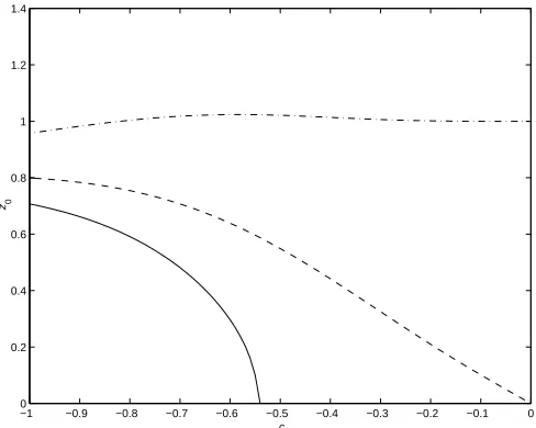
Without loss of generality we can assume that the underlying flow is propagating in the positive direction of thex-coordinate, i.e. A >0. Then (58) leads to the following restriction to the possible values ofc: c_≥1 (for the waves, moving in the direction of the flow, downstream) or ₋1_≤c <0 (for the waves, propagating upstream). The plot of the dependence of z0 on c , according to the equations (65), (66) and (67) is given on Fig.1 and Fig.2. From Fig.2 we notice that there is a region, where the function (65) is not real: c0 ≤c≤0,c0 ≈ −0.544, and therefore the CH (in this setting) is not a relevant model for these values ofc. Although the graph of (67) has a maximumz0 ≈1.0237 atc≈ −0.600. which violates the conditionz0 ≤1, we notice that in the case of upstream propagation (Fig.2) for all possible values of c one can assume z0 ≈1, i.e. equation (42) models very well the wave propagation on the surface (z0= 1) for all possible velocities.

5

Conclusions

1 2 3 4 5 6 7 8 9 10 11 12 13 0.55

0.6 0.65 0.7 0.75 0.8 0.85 0.9 0.95 1

c z0

Figure 1: Downstream propagation: plot of the dependence of z0 on c. (65) for CH – solid line; (66) for DP – dashed line; (67) for equation (43) – dash-dotted line. All cases have a horizontal asymptotez0 → √1

3 ≈0.577 asc_{→ ∞}. The CH graph has a maximumz0 ≈0.762 atc≈1.416; The DP graph has a maximumz0 ≈0.806 atc≈1.149.

−1 −0.9 −0.8 −0.7 −0.6 −0.5 −0.4 −0.3 −0.2 −0.1 0

0 0.2 0.4 0.6 0.8 1 1.2 1.4

c z0

2003), periodic solutions (Gesztesy & Holden 2003), traveling-waves (Parkes & Vakhnenko 2005), (Lenells 2005a). The construction of multi-soliton and multi-positon solutions for the Associated Camassa-Holm equation using the Darboux/B¨acklund transform is presented in (Schiff 1998), (Hone 1999) and (Ivanov, 2005b). The N-soliton solution for the DP equation was recently derived by Matsuno (2005a), the multi-peakon solutions for DP are obtained by Lundmark & Szmigielski (2003, 2005); the traveling waves – by Parkes & Vakhnenko (2004) and Lenells (2005b). There are similarities between the CH and DP equations, in a sense that they both are integrable and have a hydrodynamic derivation. However, it is interesting to notice that only CH has a geometric interpretation as a geodesic flow, cf. (Constantin & Kolev 2003), (Kolev 2004).

Acknowledgements

The author acknowledges funding from the Irish Research Council for Sci-ence, Engineering and Technology. This paper was written while the author participated in the program ”Wave Motion” at the Mittag-Leffler Institute, Stockholm, in the Fall of 2005.

References

[1] Burns, J.C. 1953 Long waves on running water. Proc. Cambridge Phil. Soc. 49, 695–706.

[2] Beals, R., Sattinger, D. & Szmigielski, J. 2003 Continued fractions and integrable systems.J. Comput. Appl. Math. 153, 47–60.

[3] Caudrey, P., Dodd, R. & Gibbon, J. 1976 A new hierarchy of Korteweg-de Vries equations, Proc. R. Soc. London A351, 407–422.

[4] Constantin, A. 1998 On the inverse spectral problem for the Camassa-Holm equation.J. Funct. Anal. 155, 352–363.

[5] Constantin, A. 2000 Existence of permanent and breaking waves for a shallow water equation: a geometric approach.Ann. Inst. Fourier (Greno-ble)50, 321–362.

[6] Constantin, A. 2001 On the scattering problem for the Camassa-Holm equation.Proc. R. Soc. Lond. A 457, 953–970.

[8] Constantin, A., Gerdjikov, V.S. & Ivanov R.I. 2006 Inverse scattering transform for the Camassa-Holm equation Inv. Problems 22, 2197-2207; nlin.SI/0603019.

[9] Constantin, A. & McKean, H.P. 1999 A shallow water equation on the circle.Commun. Pure Appl. Math. 52, 949–982.

[10] Constantin, A. & Kolev, B. 2003 Geodesic flow on the diffeomorphism group of the circle. Comment. Math. Helv.78, 787–804.

[11] Constantin, A. & Molinet, L. 2001 Orbital stability of solitary waves for a shallow water equation. Physica 157D, 75–89.

[12] Constantin, A. & Strauss, W. 2000 Stability of peakons.Commun. Pure Appl. Math.53, 603–610.

[13] Constantin, A. & Strauss, W. 2002 Stability of the Camassa-Holm soli-tons.J. Nonlinear Sci. 12, 415–422.

[14] Degasperis, A. & Procesi, M. 1999 Asymptotic integrability. In Sym-metry and perturbation theory(ed. A. Degasperis & G. Gaeta), pp 23–37, Singapore: World Scientific.

[15] Degasperis, A., Holm. D.D. & Hone, A.N.W. 2002 A new integrable equation with peakon solutions. Theor. Math. Phys.133, 1463–1474. [16] Dullin, H.R., Gottwald, G.A. & Holm, D.D. 2003 Camassa-Holm,

Korteweg-de Vries-5 and other asymptotically equivalent equations for shallow water waves. Fluid Dynam. Res. 33, 73–95.

[17] Dullin, H.R., Gottwald, G.A. & Holm D.D. 2004 On asymptotically equivalent shallow water wave equations.Physica 190D, 1–14.

[18] Fokas, A. & Fuchssteiner, B. 1981 Symplectic structures, their B¨acklund transformation and hereditary symmetries. Physica4D, 821–831.

[19] Fokas, A. & Liu, Q. 1996 Asymptotic integrability of water waves.Phys. Rev. Lett.77, 2347–2351.

[20] Gesztesy, F. & Holden, H. 2003 Soliton equations and their algebro-geometric solutions, part I: (1 + 1) -dimensional continuous models. bridge studies in advanced mathematics, volume 79. Cambridge: Cam-bridge University Press.

[22] Hone, A. 1999 The associated Camassa-Holm equation and the KdV equation.J. Phys. A: Math. Gen.32, L307-L314.

[23] Ivanov, R.I. 2005aOn the integrability of a class of nonlinear dispersive wave equations.Journal of Nonlinear Mathematical Physics12, 462–468; arXiv: nlin/0606046v1 [nlin.SI]

[24] Ivanov, R.I. 2005bConformal properties and B¨acklund transform for the Associated Camassa-Holm equation. Phys. Lett. 345A, 235-243; arXiv: nlin/0507005v1 [nlin.SI]

[25] Johnson, R.S. 1997 A modern introduction to the mathematical theory of water waves, Cambridge: Cambridge University Press.

[26] Johnson, R.S. 2002 Camassa-Holm, Korteweg-de Vries and related models for water waves. J. Fluid Mech.457, 63–82.

[27] Johnson, R.S. 2003aThe Camassa-Holm equation for water waves mov-ing over a shear flow. Fluid Dyn. Res. 33, 97–111.

[28] Johnson, R.S. 2003bOn solutions of the Camassa-Holm equation.Proc. Roy. Soc. Lond. A459, 1687–1708.

[29] Kaup, D. 1980 On the inverse scattering problem for the cubic eigen-value problem of the class φxxx+ 6Qφx+ 6Rφ =λφ. Stud. Appl. Math.

62, 189–216.

[30] Kodama, Y. 1985 On integrable systems with higher order corrections. Phys. Lett.107A, 245–249.

[31] Kolev, B. 2004 Lie groups and mechanics: an introduction.J. Nonlinear Math. Phys.11, 480–498.

[32] Lenells, J. 2005a Traveling wave solutions of the Camassa-Holm equa-tion.J. Differential Equations 217, 393–430.

[33] Lenells, J. 2005b Traveling wave solutions of the Degasperis-Procesi equation.J. Math. Anal. Appl.306, 72–82.

[34] Li, Y. & Zhang, J. 2004 The multiple-soliton solutions of the Camassa-Holm equation.Proc. R. Soc. Lond. A 460, 2617-2627.

[35] Li, Y. 2005 Some water wave equations and integrability. J. Nonlinear Math. Phys.12 (Suppl. 1), 466-481.

[36] Lundmark, H. & Szmigielski, J. 2003 Multi-peakon solutions of the Degasperis-Procesi equation. Inv. Problems19, 1241–1245.

[38] Matsuno, Y. 2005a The N-soliton solution of the Degasperis-Procesi equation.Inv. Problems 21, 2085–2101. arXiv: nlin/0511029v1 [nlin.SI] [39] Matsuno, Y. 2005b Parametric representation for the multisoliton

solu-tion of the Camassa-Holm equasolu-tion. J. Phys. Soc. Japan 74, 1983–1987; arXiv: nlin/0504055v1 [nlin.SI]

[40] Mikhailov, A.V. & Novikov, V.S. 2002 Perturbative symmetry ap-proach. J. Phys. A35, 4775–4790.

[41] Olver, P. & Jing Ping Wang 2000 Classification of integrable one-component systems on associative algebras. Proc. London Math. Soc.81, 566–586.

[42] Parker, A. 2004 On the Camassa-Holm equation and a direct method of solution I. Bilinear form and solitary waves. Proc. R. Soc. Lond. A 460, 2929-2957.

[43] Parker, A. 2005aOn the Camassa-Holm equation and a direct method of solution II. Soliton solutions.Proc. R. Soc. Lond. A 461, 3611-3632. [44] Parker, A. 2005b On the Camassa-Holm equation and a direct method

of solution III. N-soliton solutions.Proc. R. Soc. Lond. A461, 3893-3911. [45] Parkes, E. & Vakhnenko, V 2004 Periodic and solitary-wave solutions of the Degasperis-Procesi equation. Chaos Solitons Fractals 20, 1059–1073. [46] Parkes, E. & Vakhnenko, V 2005 Explicit solutions of the

Camassa-Holm equation.Chaos, Solitons and Fractals 26, 1309–1316.

[47] Sanders, J. & Jing Ping Wang 1998 On the integrability of homogenous scalar evolution equations,J. Diff. Eq.147, 410–434.

[48] Sawada, K. & Kotera, T. 1974 A method for findingN-soliton solutions of the KdV equation and KdV-like equation. Progr. Theor. Phys. 51, 1355–1367.

[49] Schiff, J. 1998 The Camassa-Holm equation: a loopgroup approach. Physica 121D, 24–43.