CORNER FORMS AND A REMAINDER INTERVAL NEWTON
METHOD
Thesis by Marcel Gavriliu
In Partial Fulfillment of the Requirements for the Degree of
Doctor of Philosophy
California Institute of Technology Pasadena, California
2005
Acknowledgements
Abstract
In this thesis we present two new advancements in verified scientific computing using interval analysis:
1. The Corner Taylor Form (CTF) interval extension. The CTF is the first interval ex-tension for multivariate polynomials that guarantees smaller excess width than the natural extension on any input interval, large or small. To help with the proofs we introduce the concept of Posynomial Decomposition (PD). Using PD we develop simple and elegant proofs showing the CTF is isotonic and has quadratic or better (local) inclusion conver-gence order. We provide methods for computing the exact local order of converconver-gence as well as the magnitude of excess width reduction the CTF produces over the natural exten-sion.
2. The Remainder Interval Newton (RIN) method. RIN methods use first order Taylor Models (instead of the mean value theorem) to linearize (systems of) equations. We show that this linearization has many advantages which make RIN methods significantly more efficient than conventional Interval Newton (IN). In particular, for single multivariate equa-tions, we show that RIN requires only order of the square root as many solution regions as IN does for the same problem. Therefore, RIN realizes same order savings in both time and memory for a significant overall improvement.
We also present a novel application of the two contributions to computer graphics: Beam
Table of Contents
Acknowledgements iii
Abstract iv
List of Figures 1
1 Introduction and Motivation 1
1.1 Benefits of Interval Computations . . . 2
1.2 Thesis Overview . . . 4
2 Review of Interval Analysis 7 2.1 A Note About Notation . . . 7
2.1.1 Interval Notation . . . 8
2.1.2 Other Notation . . . 10
2.2 Intervals and Interval Arithmetic . . . 11
2.3 Inclusion Functions and Interval Extensions . . . 15
2.3.1 Interval Valued Functions and the Range Inclusion Function . . . 15
2.3.2 Inclusion of the Range of Real Valued Functions . . . 16
2.3.3 Interval Extensions . . . 18
2.4 Inclusion of the Solution Set of Nonlinear Systems of Equations . . . 20
2.4.1 A Basic Divide and Conquer Algorithm . . . 21
2.5 Inclusion of the Solution Set of Nonlinear Optimization Problems . . . 26
2.6 Inclusion of the Solution Set of Systems of Differential and Integral Equations
using Interval Picard Iterations . . . 28
2.6.1 Definitions . . . 28
2.6.2 Interval Picard Iteration . . . 29
2.6.3 An Example . . . 30
3 Related Previous Work 33 3.1 Taylor Forms and Taylor Models . . . 33
3.1.1 Taylor Form Interval Extensions . . . 35
3.1.2 Taylor Form Chronology . . . 36
3.2 Methods for the Robust Inclusion of the Range of Multivariate Functions . . . . 37
3.2.1 Horner Forms . . . 37
3.2.1.1 Summary of Properties . . . 38
3.2.2 Centered and Mean Value Forms . . . 39
3.2.2.1 Summary of Properties . . . 40
3.2.3 Taylor Forms Revisited . . . 41
3.2.4 Bernstein Forms . . . 41
3.2.4.1 Bernstein Forms for Polynomials . . . 42
3.2.4.2 Bernstein Forms for Other Types of Functions . . . 43
3.2.4.3 Short Chronology . . . 43
3.2.4.4 Summary of Properties . . . 44
3.3 Interval Newton Methods for the Inclusion of the Roots of Nonlinear Systems of Equations . . . 44
3.3.1 Linear Interval Equations . . . 46
3.3.2 The Interval Newton Operator . . . 47
3.3.3 Preconditioning . . . 48
3.3.4 The Krawczyk Operator . . . 49
3.3.5 The Hansen-Sengupta Algorithm . . . 50
4 Corner Taylor Form Inclusion Functions 53
4.1 Introduction . . . 53
4.2 Sign-Coherent Intervals . . . 53
4.3 Sign-Coherent Interval Decomposition . . . 55
4.4 Posynomials . . . 56
4.5 The Posynomial Decomposition of a Polynomial . . . 57
4.6 Taylor Form Excess Width is Due to One Interval Minus Operation . . . 59
4.7 Reduction to the Non-Negative Quadrant . . . 60
4.8 Corner Taylor Forms With Interval Coefficients . . . 62
4.8.1 The Corner Taylor Form Always Has Less Excess Width Than the Nat-ural Extension . . . 62
4.8.2 Isotonicity of the Corner Taylor Form . . . 64
4.9 Corner Taylor Forms With Real Coefficients . . . 68
4.9.1 The Magnitude of the Improvement Over Natural Extensions . . . 69
4.9.2 Convergence Properties . . . 72
4.10 Examples and Results . . . 74
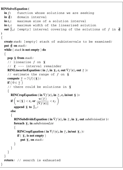
5 Remainder Interval Newton Methods 91 5.1 The RIN Algorithm for Roots of Multivariate Nonlinear Equations . . . 92
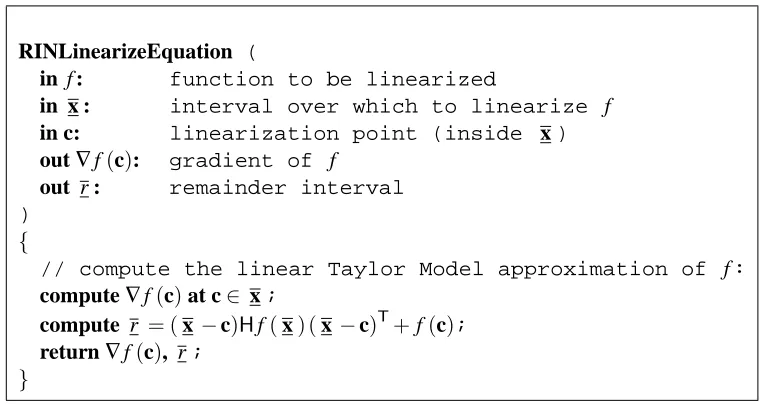
5.1.1 Linearization . . . 94
5.1.2 Cropping . . . 96
5.1.3 Subdivision . . . 102
5.1.4 Convergence of the RIN Algorithm . . . 104
5.2 The RIN Algorithm for Roots of Square Systems of Nonlinear Equations . . . . 105
5.2.1 Linearization . . . 105
5.2.2 Cropping . . . 107
5.2.3 Tightening . . . 108
5.3 RIN vs. Martin Berz’s Inversion . . . 109
5.5 Examples and Performance . . . 110
5.5.1 Polynomial Equations . . . 110
5.5.2 Polynomial Systems . . . 111
6 An Application: Beam Tracing for Implicit Surfaces 134 6.1 Introduction . . . 134
6.2 Previous Work . . . 137
6.2.1 Review: Ray/Implicit Surface Intersection in One Variable . . . 137
6.2.2 Methods that Do Not Guarantee Solutions . . . 138
6.2.3 Methods that Guarantee Solutions Along a Ray . . . 139
6.2.4 Methods that Guarantee Solutions Inside a Pixel . . . 141
6.3 Beam Tracing Implicit Surfaces . . . 141
6.3.1 Beams . . . 141
6.3.2 Beam-Surface Intersection . . . 142
6.3.3 Computing the Illumination . . . 142
6.3.4 Generating Reflected/Refracted Beams . . . 143
6.3.5 Making Beam Tracing Work . . . 143
6.4 Results and Conclusions . . . 145
6.5 Future Work . . . 148
7 Conclusion 149
List of Figures
2.1 A simple divide and conquer algorithm for solving nonlinear systems of equations using interval analysis. The values between square brackets listed next to variable declarations represent initial values. Using a FIFO queue instead of the LIFO stack usually increases storage requirements. . . 22 2.2 Plot of an interval covering produced by the divide and conquer algorithm in
fig-ure 2.1, using the natural inclusion function andε=2−4. The interval covering contains 12,407 solution intervals and has a quality factor of only 0.0571. The al-gorithm performed a total of 29,105 iterations which took 84.281 seconds (Math-ematica 5, P4-2.2GHz). The time/quality cost is 1,474.858 seconds. Compare this with figure 2.3. . . 23 2.3 Plot of an interval covering produced by the divide and conquer algorithm in
fig-ure 2.1, using a Midpoint Taylor Form inclusion function andε=2−4. The interval covering contains 788 solution intervals and has a quality factor of 0.8997. The algorithm performed a total of 4,951 iterations which took 63.016 seconds (Math-ematica 5, P4-2.2GHz). The time/quality cost is 70.038 seconds. Compare this with figure 2.2. . . 24 2.4 A simple branch and bound nonlinear optimization algorithm using interval
analy-sis, after Moore and Skelboe. The subroutines used in the algorithm are briefly described in section 2.5.1. . . 27 2.5 An example of contracting Taylor Models generated using interval Picard
3.1 The generic Interval Newton algorithm for solving nonlinear systems of equations. The values between square brackets listed next to variable declarations represent initial values. . . 45 3.2 A recursive Interval Newton contraction algorithm for solving nonlinear systems
of equations. This function replaces the generic NewtonContraction in the Inter-val Newton algorithm in Figure 3.1. . . 47 3.3 A recursive Krawczyk contraction algorithm for solving nonlinear systems of
equations. This function replaces the generic NewtonContraction in the Inter-val Newton algorithm in Figure 3.1. . . 50 3.4 A recursive Hansen-Sengupta contraction algorithm for solving nonlinear systems
of equations. This function replaces the generic NewtonContraction in the Inter-val Newton algorithm in Figure 3.1. . . 51
4.1 The range of the polynomial p(x)on the interval[1,2]isR(p) ([1,2]). The exact value of the range on an interval can be difficult to compute. . . 64 4.2 The natural extension N(p) greatly overestimates the range. Proposition 4.6.1
proves that the width of the computed bound is equal to the sum of widths of the ranges of p⊕and p , the P and N-posynomials of the MacLaurin form of p. . . 65 4.3 The Corner Taylor Form, Tc(p), produces improved bounds as shown in
Theo-rem 4.9.1. The width of the Corner Taylor Form is equal to the sum of the widths of the ranges of T p⊕ and T p , the P and N-posynomials of the Taylor Form of
p(x)expanded at x=1. Note that T p⊕ and T p have smaller ranges than the P and N-posynomials, p⊕ and p , of the MacLaurin form (see figure 4.2). There-fore, the Corner Taylor Form inclusion function,Tc(p) ([1,2]), produces bounds
with significantly less excess width when compared to the natural inclusion func-tionN(p) ([1,2]). . . 66 4.4 The magnitude of the improvement w(N(p))−w(Tc(p)) can be computed in
4.5 Regions in gray indicate possible roots of the fifth order Taylor multino-mial MacLaurin<5,5>(cos 2x sin 3y+sin 3x cos 2y−cos 2x cos 3y+sin 3x sin 2y) = 0 computed using the natural inclusion function. The search process converges very slowly due to the large excess width of the natural inclusion function, retain-ing many superfluous solution regions. The quality factor is only 0.0571. . . 80 4.6 Roots of the same multinomial as in figure 4.5 computed using the Midpoint
Tay-lor Form inclusion function. The search process converges quickly once the size of the regions fall under a certain threshold. There is still a fair amount of work being done to eliminate regions where there are no roots as shown, for example, in the upper right corner. Several subdivisions are needed before the region can be declared root free. The quality factor is 0.8997. Compare with figure 4.7. . . 81 4.7 Roots of the same multinomial as in figures 4.5 and 4.6 computed using the Corner
Taylor Form inclusion function, Tc(f). Notice that the Corner Taylor Form is
more accurate than the Midpoint Taylor Form for large input regions. The region in the upper right corner is declared root free very early in the subdivision process. The quality factor is 0.8821. Compare with figure 4.6. . . 82 4.8 Plot of the solution regions produced by divide and conquer with Midpoint Taylor
Forms on larger domains. The domain is[−100,100]2. The algorithm found 4,950 solution regions in 36,899 iterations which took 514.765 seconds (Mathematica 5 time). Note that there is a considerable amount of work being done away from the solutions. Compare with figure 4.9. . . 83 4.9 Plot of the solution regions produced by divide and conquer with Corner Taylor
4.10 Plot of the solution regions produced by divide and conquer with Midpoint Taylor Forms on larger domains for a different function. The domain is[−20,20]2. The algorithm finished in 1,099 iterations which took 5.016 seconds (Mathematica 5 time). Compare with figure 4.11. . . 85 4.11 Plot of the solution regions produced by divide and conquer with Midpoint Taylor
Forms on larger domains for a different function. The domain is[−20,20]2. The algorithm finished in 543 iterations which took 2.531 seconds (Mathematica 5 time). Compare with figure 4.10. . . 86 4.12 Plot of the solution regions produced by divide and conquer with Midpoint Taylor
Forms on even larger domains. The domain is increased to[−2000,2000]2. The algorithm finished in 4,503 iterations which took 21.093 seconds (Mathematica 5 time). Compare with figure 4.13. . . 87 4.13 Plot of the solution regions produced by divide and conquer with Midpoint
Tay-lor Forms on even larger domains. The domain is increased to[−2000,2000]2. The algorithm finished in 827 iterations which took 3.875 seconds (Mathematica 5 time). Once again we observe the fastest possible convergence of binary subdi-vision. Compare with figure 4.12. . . 88 4.14 Logarithmic plot of the number of iterations required by various interval solution
methods versus the size of the solution intervals expressed as a power of 2. . . 89 4.15 Logarithmic plot of the CPU time (Mathematica 5.0) required by various interval
solution methods versus the size of the solution intervals expressed as a power of 2. 90
5.1 The Remainder Interval Newton algorithm for solving a single nonlinear equation. 93 5.2 The Remainder Interval Newton linearization algorithm for solving a single
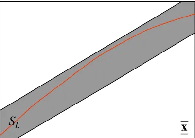
non-linear equation. . . 95 5.3 An example of a solution set of the linearized equation 5.4. The red curve
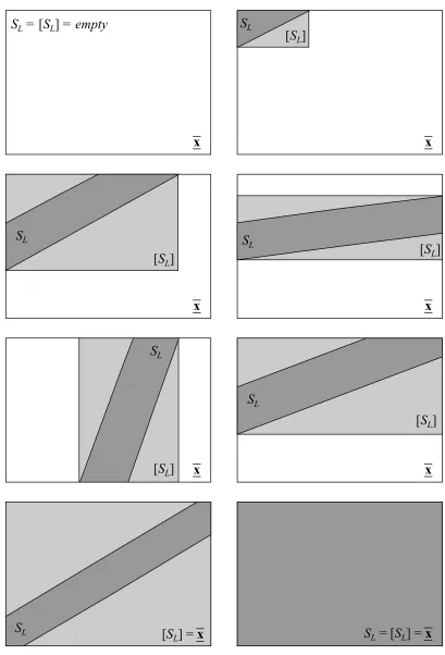
5.4 Several ways in which the linearized solution SLcan intersect an interval x .[[SL]]
is the interval convex hull of the intersection. . . 97 5.5 The Remainder Interval Newton cropping algorithm for solving a single nonlinear
equation. . . 98 5.6 The Remainder Interval Newton subdivision algorithm for solving a single
non-linear equation. . . 102 5.7 The Remainder Interval Newton algorithm for solving square systems of nonlinear
equations. . . 106 5.8 The Remainder Interval Newton linearization algorithm for solving square
sys-tems of nonlinear equations. . . 107 5.9 The Remainder Interval Newton cropping algorithm for solving square systems of
nonlinear equations. . . 108 5.10 The Remainder Interval Newton tightening algorithm for solving square systems
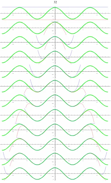
of nonlinear equations. . . 109 5.11 The solution set of the 5th order bivariate Taylor expansion around the point(1,1)
of the function f(x,y) =cos 3x(sin 2y+cos 2y) +cos 2x(sin 3y−cos 3y)inside the interval[−π,π]×[−π,π]. The curves are computed with RIN and are composed of 3,541 linearized solution regions of width at most 2−10. . . 113 5.12 Logarithmic plot of the number of iterations required by various interval solution
methods versus the size of the solution intervals expressed as a power of 2. . . 114 5.13 Logarithmic plot of the CPU time (Mathematica 5.0) required by various interval
solution methods versus the size of the solution intervals expressed as a power of 2. 115 5.14 Logarithmic plot of the number of solution regions produced by various interval
5.15 Plot of the solution regions produced by Divide and Conquer with Naive Natural Extension. The solution box width is less than 2−4. The algorithm found 12,407 solution regions in 29,105 iterations which took 84.281 seconds (Mathematica 5 time). Note that it would have taken considerably more time to produce the same level of solution separation that was possible using the more advanced methods shown on the following pages. . . 117 5.16 Plot of the solution regions produced by Divide and Conquer with Midpoint Taylor
Forms. The solution box width is less than 2−4. The algorithm found 788 solution regions in 4,951 iterations which took 63.016 seconds (Mathematica 5 time). . . . 118 5.17 Plot of the solution regions produced by Divide and Conquer with Corner Taylor
Forms. The solution box width is less than 2−4. The algorithm found 807 solution regions in 4,841 iterations which took 61.312 seconds (Mathematica 5 time). . . . 119 5.18 Plot of the solution regions produced by the Interval Newton method with
Mid-point Taylor Forms. The solution box width is less than 2−5. The algorithm found 1,557 solution regions in 5,067 iterations which took 67.656 seconds (Mathemat-ica 5 time). . . 120 5.19 Plot of the solution regions produced by the RIN method with Midpoint Taylor
Forms and binary subdivision (not using our special subdivision). The linearized solution width is less than 2−5. The algorithm found 947 solution regions in 3,039 iterations which took 69.64 seconds (Mathematica 5 time). . . 121 5.20 Plot of the solution regions produced by the RIN method with Midpoint Taylor
Forms and RIN subdivision. The linearized solution width is less than 2−5. The algorithm found 588 solution regions in 2,382 iterations which took 43.328 sec-onds (Mathematica 5 time). . . 122 5.21 Plot of the solution regions produced by the RIN method with Midpoint Taylor
5.22 Plot of the solution regions produced by the RIN method with Corner Taylor Forms, RIN subdivision, and non-box solutions. The linearized solution width is less than 2−5. The algorithm found 605 solution regions in 2,982 iterations
which took 39.469 seconds (Mathematica 5 time). . . 124 5.23 Plot of the solution regions produced by the RIN method with Corner and
Mid-point Taylor Forms (switch from CTF to MTF when intervals have width less than 1), RIN subdivision, and non-box solutions. The linearized solution width is less than 2−5. The algorithm found 353 solution regions in 1,704 iterations which took 25.197 seconds (Mathematica 5 time). . . 125 5.24 Interval Newton without tightening. Solutions of the system of polynomials 5.5.2
over [−π,π]2. Solution interval width is less than 2−4. The algorithm found 96 solution regions in 1,939 iterations which took 72.8 seconds (Mathematica 5, [email protected].) . . . 126 5.25 Interval Newton with tightening. Solutions of the system of polynomials 5.5.2
over [−π,π]2. Solution interval width is less than 2−4. The algorithm found 96 solution regions in 1,651 iterations which took 63.5 seconds (Mathematica 5, [email protected].) . . . 127 5.26 Remainder Interval Newton without tightening. Solutions of the system of
polyno-mials 5.5.2 over[−π,π]2. Solution interval width is less than 2−4. The algorithm found 96 solution regions in 1,403 iterations which took 46.3 seconds (Mathemat-ica 5, [email protected].) . . . 128 5.27 Remainder Interval Newton with tightening. Solutions of the system of
5.28 Interval Newton without tightening. Solutions of the system of polynomials 5.5.2 over[−2π,2π]2. Solution interval width is less than 2−4. The algorithm found 96 solution regions in 4,067 iterations which took 157.125 seconds (Mathematica 5, [email protected].) . . . 130 5.29 Interval Newton with tightening. Solutions of the system of polynomials 5.5.2
over[−2π,2π]2. Solution interval width is less than 2−4. The algorithm found 96 solution regions in 3,331 iterations which took 129.75 seconds (Mathematica 5, [email protected].) . . . 131 5.30 Remainder Interval Newton without tightening. Solutions of the system of
poly-nomials 5.5.2 over[−2π,2π]2. Solution interval width is less than 2−4. The al-gorithm found 96 solution regions in 2,787 iterations which took 95.687 seconds (Mathematica 5, [email protected].) . . . 132 5.31 Remainder Interval Newton with tightening. Solutions of the system of
polynomi-als 5.5.2 over[−2π,2π]2. Solution interval width is less than 2−4. The algorithm found 96 solution regions in 2,099 iterations which took 71.891 seconds (Mathe-matica 5, [email protected].) . . . 133
6.1 Rendering of a complex implicit model with thin, hair like features. Top, the whole scene. Bottom, detail views of one of the thin features of the surface. Left, ray traced images, above, antialiased and below, not antialiased; the rays sometimes miss the hair like features causing them and their shadows to appear discontinuous.
Right, beam traced images; the thin features and the shadows they cast are always
continuous and free of pixel dropouts. . . 135 6.2 Applying multiple rotation transformations to a region can artificially increase its
size. This artifact is known as the wrapping effect. . . . 144 6.3 Rendering of a blobby flake. The model is comprised of 91 blended elliptic blobby
primitives. Left, Gaussian blobbies. Right, polynomial blobbies. . . 145 6.4 Rendering of a very complex implicit model with thin, hair like features. The
Chapter 1
Introduction and Motivation
Over the last decade we have observed an increasing trend towards replacing costly real-life tests and experiments with computer simulations. From automobile crash tests to spacecraft trajectory planning to DOE’s Advanced Simulation and Computing project (formerly known as ASCI) decisions that strategically affect our day to day lives are made based on the results of computer simulations. This emerging trend prompts the need for reliable and efficient self-verified computing methods that can guarantee prediction of results one hundred percent.
Traditional numerical computing uses IEEE floating point arithmetic (IEEE 754 standard). This floating point standard is widely supported in hardware; highly optimized math libraries (such as Intel’s Performance Libraries) are readily available. Unfortunately, floating point pro-cedures are not sufficient to guarantee correct results in all cases, as is demonstrated by a classic example by Rump, which we briefly review in the next section. Rump provides a simple ratio-nal expression designed so that evaluation using floating point fails to produce the correct result even when the number of digits of precision is doubled, and doubled again. This simple example shows that no algorithm using floating point alone can be relied on to make strategic decisions without risk.
Interval analysis was formally introduced by R. E. Moore in the 1960’s, see [Moore 1962,
1.1
Benefits of Interval Computations
Although not new, interval analysis has not found the widespread acceptance its creators had hoped for. The common belief is that there are faster, more straightforward methods that can account for rounding and other types of errors. For example, it is common practice to compute results independently in both single and double precision floating point and compare the digits of the two results. If the significant digits agree up to a certain precision then the matching digits are considered correct. However, it is relatively easy to design examples where the above method breaks. One such case is the classic example by Rump who, in 1988, published an expression for which numerical evaluation with floating point arithmetic gave erroneous and misleading results. When evaluating Rump’s expression with increasing numbers of digits the results seemed stable as they agreed in their first few significant digits. However, as it turns out, all the digits were incorrect and, although the computed answer was relatively far from zero, it failed to even capture the correct sign. Rump’s example is not reproducible on modern IEEE 754 computers. Fortunately, the following expression due to Walster and Loh, reproduced from [Hansen and Walster 2003], produces a similar outcome, this time using IEEE 754 floating point arithmetic:
f(x,y) = (333.75−x2)y6+x2(11x2y2−121y4−2) +5.5y8+ x 2y
For x=77,617 and y=33,096 one would obtain the following results:
32 bits: f(x,y) = 1.172604
64 bits: f(x,y) = 1.1726039400531786
128 bits: f(x,y) = 1.172603940053178618588349045201838
In spite of their agreement in the first digits all three results are wrong. The correct answer is:
Evaluation using even the simplest form of interval analysis (natural extension) produces a wide interval that contains the correct value above. While not directly providing a better (point) an-swer, interval evaluation alerts us to the numerical instability of the expression and suggests that higher-accuracy methods need to be employed if the correct answer is to be computed.
Several real world examples of disasters caused by numerical instability of floating point are documented by Douglas N. Arnold on his website at:
http://www.ima.umn.edu/∼arnold/disasters/,
as well as in [Hansen and Walster 2003]. All these disasters could have been easily avoided if interval analysis were used for validation.
Another common complaint is that interval methods are too slow to be useful in practice. While it is true that computing with intervals is inherently slower than computing with floating point numbers we have to make certain that we are comparing apples with apples. Often times, interval methods are the only ones capable of reliably solving the problem at hand. This is the case, for example, when solving general nonlinear global optimization problems. Another example is the computation of global solution sets of underdetermined systems of nonlinear equations. In such cases there is no competing floating point method—interval analysis is the fastest method available.
In the cases where a competing (non error bounding) floating point method does exist, meth-ods using interval analysis will naturally be slower. The slowdown factor depends on many factors and varies greatly. Properly optimized interval algorithms are generally no more than one order of magnitude slower than their float counterparts. This is often a reasonable price to pay for the guaranteed error bounds produced by interval analysis. As interest in intervals grows so will the degree of refinement of implementation and the gap will continue to narrow.
the limits of Moore’s Law and we cannot count on CPU speeds doubling every 18 months. As a result, the intrinsic efficiency of the algorithms used becomes increasingly more important.
Use of the classic natural extension coupled with simple spatial subdivision is slow and produces unusable results for all but the simplest of problems, as can be seen in the examples in chapter 4. Such meager performance can be enough to convince people that all of interval analysis is inefficient and should be avoided. Fortunately, this is not the case with state of the art methods such as higher order interval extensions (Centered and Taylor Forms, Bernstein Forms, Taylor Models, etc.) coupled with quadratically convergent Interval Newton—very sharp bounds can be computed in reasonably fast times at the expense of rather complicated implementation costs.
The methods introduced in this thesis further improve the efficiency of interval methods. Corner Taylor Forms are the first interval extensions to guarantee smaller excess width than the natural extension when evaluated on large intervals while preserving the quadratic conver-gence properties of the Taylor Form. Remainder Interval Newton improves over classic Interval Newton with a special subdivision algorithm that extends its applicability to non-square systems while helping improve efficiency by a factor of the square root (fewer steps).
1.2
Thesis Overview
In this section we give a structural overview of the thesis.
The thesis has two parts. The first part is comprised of chapters 2 and 3. Its main objective is to provide an easy to read overview of the previous state of the art in interval analysis and to provide some of the motivation for the contributions we present in the second part of the thesis. Therefore, we have omitted all the proofs and instead concentrated on the relationships between the many concepts we discuss.
functions and natural interval extensions in section 2.3. Next we take a look at various solution methods that use interval analysis. Section 2.4 reviews the basic divide and conquer algorithm for solving nonlinear systems of equations. Finally, section 2.5 presents a simple branch and bound algorithm for solving general nonlinear optimization problems.
Chapter 3 extends the concepts introduced in the previous chapter and presents the most important state of the art methods in use in interval analysis today. We begin with a discussion of Taylor Forms and Taylor Modes in section 3.1. In section 3.2 we review some of the higher order types of inclusion functions such as the Centered (Slope) Form and the Bernstein Form. Finally, section 3.3 discusses some of the most important variants of Interval Newton for solving systems of nonlinear equations.
Part two of this thesis details our contributions to the state of the art. We give proofs of all the new results as well as some new, more elegant, proofs of results that are already known.
Form has many of the desirable properties of the more general Taylor Form interval extension. In section 4.8.2 we prove isotonicity (the interval analytic equivalent monotonicity). Finally, in section 4.9.2 we develop a novel proof showing the excess width of the Corner Taylor Form has at least quadratic order of convergence or better. In particular, we show how to compute the order of convergence in closed form as a function of the expression of the polynomial and the input interval under investigation. These formulas can be used once again to make real-time decisions about which inclusion functions to use. The proofs are facilitated by a new, surprisingly simple and powerful tool called Posynomial Decomposition. Posynomial Decomposition (PD) is described in section 4.5. The chapter concludes with several simple examples.
Chapter 5 details the second contribution of this thesis. We present a new method for solving systems of nonlinear equations called the Remainder Interval Newton method (RIN for short). In place of the commonly used mean value theorem, RIN employs a first order Taylor expansion with interval remainder terms (a.k.a. first order Taylor Models) to linearize the system of equa-tions, see section 5.1.1. Another important component of the RIN method for underdetermined systems is a new subdivision method designed to maximize the benefits of the linearization process, see section 5.1.3. This subdivision scheme allows efficient pruning of regions where solutions are known not to exist. It also provides the option to enclose the solution set with solution-aligned polyhedral regions thereby producing a significant reduction in the number of regions needed to cover a (non point) set of solutions. The new subdivision method further im-proves the convergence order of the RIN method by a factor of the square root of the original number of steps. In practice we observe several orders of magnitude reduction in the total num-ber of steps as well as the numnum-ber of solution regions returned, see section 5.5. In section 5.2 we discuss the RIN algorithm for solving square systems of nonlinear equations, with examples shown in section 5.5.
Chapter 2
Review of Interval Analysis
In this chapter we review some of the fundamental definitions and properties of interval analysis that will be used throughout this thesis.
For more in depth discussion of topics related to interval analysis we refer the reader to the books by Moore [Moore 1979], Alefeld and Hertzberger [Alefeld and Herzberger 1983], Hansen [Hansen 1992] and more recently with Walster [Hansen and Walster 2003], Neumaier [Neumaier 1990], and Jaulin et al. [Jaulin et al. 2001].
2.1
A Note About Notation
In this thesis we introduce a new system of notation for interval quantities which we feel is clearer and more convenient than other notation systems currently found in the interval analysis literature. The reason for introducing new notation is our desire for a system that interferes as little as possible with current de facto mathematical notation yet is simple, uncluttered and clearly identifies any interval quantities present in formulas.
We looked for notation that can be easily employed in handwritten text, thus ruling out the use of typographical enhancements—such as bold letters representing intervals—that have been previously proposed.
cause a lot of confusion in formulas where both intervals and matrices (or sets) are present simultaneously.
Another system identifies interval quantities by enclosing them in square brackets, i.e. x is a real and[x]is an interval. While this notation avoids confusion with matrix and set notation and is handwriting friendly, we feel it adds unnecessary bulk to formulas and can be confused for “just” parentheses.
After many experiments we came to the solution of using simultaneous overbars and under-bars to represent interval quantities. This notation is consistent with the current use of overunder-bars and underbars to respectively represent the upper and lower bounds of intervals. Since an inter-val is composed of both its upper and lower bounds, it was only natural to visually merge the two into the symbolic representation of the interval.
2.1.1 Interval Notation
In this thesis, real numbers are denoted by lowercase letters, e.g. x,a,u∈R. The set of all closed real intervals is denoted byIR. Members ofIRare denoted by lowercase letters with over and underbars, e.g. x = [x0,x1], a,u ∈IR. For emphasis, vectors are denoted by bold letters, e.g. x, a,u∈Rn are vectors of reals, and x,a,u ∈
IRn are vectors of intervals. The components of a vector are marked with subscripts, e.g. xi, yj. Matrices are denoted with capital letters as
usual, while interval matrices have over and underbars: A∈Rm×n,B ∈
IRm×n.
In summary:
Real scalar: x,
Scalar interval (older notations: X,[x],x): x,
Real vector: x,
Vector interval: x,
i-th component of real vector: xi,
i-th component of interval vector: xi,
Real matrix: M,
Interval matrix: M,
(i,j)-th component of real matrix: Mi j,
(i,j)-th component of interval matrix: Mi j,
Real valued function: f(x),
Interval valued function: f (x),
Generic inclusion function of f : I(f),
Generic inclusion function of f (evaluated on x ): I(f) (x),
Natural extension of f : N(f),
Natural extension of f (evaluated on x ): N(f) (x).
2.1.2 Other Notation
In the following chapters we need to clearly distinguish not only between different functions but also between different expressions of the same function. For the sake of clarity we have chosen a somewhat verbose notation which uses common English names for the expressions in question.
A generic expression of a function f will be denoted by:
Generic expression: Expression(f).
Note that the expression is itself a function. Evaluation of the expression at a point x is written:
Evaluation of a generic expression: Expression(f) (x).
When a function has a natural (or canonical) expression we denote it by:
Natural (canonic) expression: Natural(f) (x).
As an example, we list the names of some common expressions of polynomials (in evaluation form) below:
Horner factoring: Horner(f) (x),
Taylor expansion: Taylor(f,c) (x),
MacLaurin expansion: MacLaurin(f) (x),
Horner-Taylor expansion: Horner-Taylor(f,c) (x),
Bernstein expansion: Bernstein(f) (x),
To facilitate writing expressions of multivariate functions we use the following notation:
Multi-index: i ∈ Nn,
Vector factorial: i! =
n
∏
k=1
ik!,
Vector binomial coefficients:
n i = n
∏
k=0 nk ik ,Vector power: xi =
n
∏
k=1
xik k,
Vector partial derivative: p(i)(x) = ∂
i1+...+in
∂i1x
1...∂inxn
p(x).
2.2
Intervals and Interval Arithmetic
A real valued interval represents the closed set of real numbers contained between a lower bound
x and an upper bound x :
Interval: x = [x,x] ={x| x ≤x≤ x}.
Intervals with x = x are called thin, point or degenerate intervals, while intervals with x < x
are called thick or proper intervals.
If 0≤ x the interval is called a positive interval, and we write x >0. Conversely, if x ≤0 we call the interval a negative interval, and write x <0. Positive or negative intervals are the two types of sign coherent intervals. If x =0 or x =0 we call the interval a zero-bound interval. A zero-bound positive interval is called a zero-positive interval. Similarly, a zero-bound negative interval is called a zero-negative interval.
Positive interval: x >0 iff x >0,
Negative interval: x <0 iff x <0,
Zero-positive interval: x ≥0 iff x =0,
A metric (distance function) onIRcan be defined as follows:
Metric (distance): q x,y=sup | x −y |,| x −y |
.
It is straightforward to verify that the above operator satisfies all the requirements of a metric. Therefore, one can define convergent series of intervals in the usual fashion:
Convergent sequence: lim
i→∞hxii= x iff limi→∞q(xi,x) =0. Some common unary operators on a real interval x are defined as follows:
Midpoint: m(x) = x +x
2 ,
Corner: c(x) =
0 , if 0∈ x x , if x >0
x , if x <0
Width: w(x) = x− x,
Radius: rad(x) = x −x 2 ,
Absolute Value: |x| = {|y| | x ≤y≤ x},
Mignitude: mig(x) = min|x|,
Magnitude: mag(x) = max|x|,
Sign: sgn(x) =
−1 , if x ≤0 0 , if x <0< x
+1 , if x ≥0
,
If S is a set of real numbers we denote its one-dimensional convex hull by[[S]]. Obviously:
Interval Hull: [[S]] = [inf(S),sup(S)],
is a closed interval.
The corresponding vector operators are defined component wise. For example, the vector corner operator is:
Vector Corner: (c(x))k = c(xk).
We do not define the sign of an interval vector.
The usual unary and binary arithmetic operations are defined as follows:
Negation: −x = [−x,−x],
Addition: x +y =
x +y,x +y,
Subtraction: x −y = x −y,x −y,
Multiplication: x y = x y,x y,x y,x y ,
Division: x
y =
""
x y,
x y,
x y,
x y
##
.
Note that for the above definition of division to work y must not contain zero. It is possible to extend the definition of division to include cases where zero is a member of y ; examples can be found in the literature.
We also define:
Positive Integral Power: xn =
[xn,xn],if n is odd or x is positive |x|n,if n is even
,
Negative Integral Power: x−n = 1
xn.
multiplications in favor of the above definition. The above integral power operator avoids the excess width introduced by repeated multiplication, as illustrated in the following example:
[−2,3]2 = [0,9] = {y=x2|x∈[−2,3]},
[−2,3] [−2,3] = [−6,9] = {y=x1x2|x1,x2∈[−2,3]}
Note that the power operator (top) returns the exact range of values while the same expression evaluated through repeated multiplication (bottom) can suffer from significant overestimation. The overestimation is due to the fact that interval multiplication as defined above assumes there is no correlation between the two factors being multiplied together.
Interval addition and multiplication exhibit the following algebraic properties:1
Commutativity: x +y = y +x, x y = y x,
Associativity: (x +y) + z = x + (y +z), (x y)z = x(y z),
Neutral Element: 0+x = x, 1·x = x.
Unfortunately, multiplication of intervals is not distributive over addition as it is with real numbers. A subdistributive law holds:
Subdistributivity: x y +z ⊆ x y +x z.
It is useful to identify the special cases where distributivity does hold: Distributivity holds:
x y ± z
= x y ±x z if x = x (thin factor),
x y + z= x y +x z if y ≥0 and z ≥0 (non-negative terms),
x y + z= x y +x z if y ≤0 and z ≤0 (non-positive terms),
x y − z
= x y −x z if y ≥0 and z ≤0 (non-negative terms variation),
x y − z= x y −x z if y ≤0 and z ≥0 (non-positive terms variation),
x y ± z= x y ±x z if x ≥0, y =0 and z =0
(positive factor, zero-straddling terms),
x y ± z= x y ±x z if x ≤0, y =0 and z =0
(negative factor, zero-straddling terms).
The proofs are straightforward and can be found in most texts on interval analysis, such as [Neumaier 1990].
2.3
Inclusion Functions and Interval Extensions
In this section we review some of the concepts associated with interval valued functions and their use for computing bounds for the range of real valued functions over interval domains.
2.3.1 Interval Valued Functions and the Range Inclusion Function
An interval valued function is a mapping from a set S to the intervalsIR:
An example of an interval valued function on the reals is the floating point bound function:
FP-bounds: FP :R→IR,FP (x) = [x∗,x∗],
where x∗ is the largest floating point number smaller than or equal to x, and x∗is the smallest floating point number greater than or equal to x.
Another example of an interval valued function, this time on intervals, is the range inclusion
function associated with a continuous real valued function f :R→R and denoted by R(f): IR→IR:
Range (continuous case): R(f) (x) ={y|(y= f(x))∧(x∈ x)}.
The range can be defined for discontinuous functions as well, using the interval hull of the range set, as follows:
Range (discontinuous case):R(f) (x) =
hh
{y|(y=f(x))∧(x∈ x)}ii.
An interval valued function is continuous if for any convergent sequencehxii(orhxiiif the
domain isR) the sequence of intervals f (xi)
(or
f (xi)
) converges as well.
2.3.2 Inclusion of the Range of Real Valued Functions
Using the range inclusion function defined in the previous section it is straightforward to design algorithms for solving many important problems, such global nonlinear optimization. Unfortu-nately, the range inclusion function is often not computable.
It turns out that computing a superset of the range inclusion function is usually sufficient, provided it has certain characteristics. We call these types of interval valued functions inclusion
functions. As the name suggests, the value of an inclusion function over some interval x in the
domain is an interval in the codomain that includes the range of the function over the interval x :
or, equivalently:
Inclusion Property: f(x)∈I(f) (x) for∀x ⊆D and∀x∈ x,
where D is the domain of f . An important class of inclusion functions are the inclusion isotone inclusion functions which satisfy the following property:
Inclusion Isotonicity:I(f) (x)⊆I(f) y
for∀x ⊆ y ⊆D.
With the above definitions many different classes of inclusion functions can be defined for any given function f , the range being the “tightest” and most useful, while the inclusion function that always returns[−∞,∞]is the “widest” but also not useful at all. We define a metric, called
excess width, for measuring how close a given inclusion function is to the range:
Excess width:∆W(I(f)) (x) =w(I(f) (x))−w(R(f) (x)).
Obviously, the excess width is a non-negative real valued function with interval arguments; the smaller the excess width is over some interval x the better the inclusion function over x is. Another measure of overestimation is the excess width ratio, which gives information about the excess width relative to the size of the arguments:
Excess width ratio:∆WR(I(f)) (x) =∆W(I(f)) (x) w(x) .
Yet another measure for overestimation of the range is the excess width range ratio, which gives information about the excess width relative to the size of the range itself:
Excess width range ratio:∆WRR(I(f)) (x) =∆W(I(f)) (x) w(R(f) (x)) .
func-tions whose excess width goes to zero in this case and in fact some authors require this property in the definition of the inclusion function. If this is the case, we define the inclusion order of an inclusion function to be the order of convergence of the excess width when evaluated on a sequence of intervals convergent to a point:
Inclusion order:
O
I(f)
=
O
∆W(I(f)) (xi)
xi→x .
2.3.3 Interval Extensions
We come to the question of obtaining an expression of an inclusion function from some given expression of a function f . If the expression of f is formed from compositions of the four basic arithmetic operations {+,−,×,÷} and integer powers, this turns out to be easy: replace all occurrences of real variables xi with interval variables xi and all the real operations with the
corresponding interval operations and what you get is the expression of an inclusion function. This is the statement of the fundamental theorem of interval analysis. The process of obtaining the expression of an inclusion function from the expression of the original function is called
interval extension, see [Moore 1979]. Given some expression we write the interval extension
simply as an evaluation with interval coefficients:
Interval extension: Expression(f) (x) is the interval extension of Expression(f) (x).
The above definitions cover interval extensions of rational functions. However, interval ex-tensions can be generalized to include other types of primitives. First, we define some composi-tion rules:
Function composition 1: Expression(f) (Expression(g) (x)) is an inclusion function of f◦g.
can obtain an inclusion function of r◦f and f◦r as follows:
Function composition 2: Expression(r) (I(g) (x))is an inclusion function of r◦g,
Function composition 3: I(g) (Expression(r) (x))is an inclusion function of g◦r.
We can summarize the composition rules above into the following rule:
Function composition:I(f) (I(g) (x)) is an inclusion function of f◦g.
The proofs are straightforward. Note that the composition rules also allow the computation of inclusion functions of algorithmically (recursively) defined functions.
Inclusion functions for many elementary functions can be easily defined and are detailed in the literature. These include square, cubic and higher roots, trigonometric and inverse trigono-metric functions, logarithms and exponentials, etc. Thus, using the composition rules, inclusion functions for a large variety of complicated functions can be easily obtained.
Most functions have a standard expression—an expression that is most often used. The inclusion functions generated from these expressions are called natural inclusion functions, or
natural extensions. For example, given a multivariate polynomial p, the natural extension2 is defined as:
Natural extension for polynomials:N(p) (x) =MacLaurin(p) (x).
The natural extension of cos((x−1)(x−3))is:
N(cos((x−1)(x−3))) (x) =cos x2−4 x+3
.
In general, inclusion functions obtained through interval extension from different expressions of the same function f are not the same, even when evaluated with infinite precision. This is unlike the real case where different expressions evaluate to the same value of f(x). One of the 2other authors choose to define the natural extension of polynomials as Horner(p) (x). This definition yields
main interests of interval analysis is in finding expressions of functions that generate “better” inclusion functions, see chapters 3 and 4.
2.4
Inclusion of the Solution Set of Nonlinear Systems of Equations
In this section we review some basic algorithms for robustly computing roots of nonlinear equa-tions of the form:
f(x) =0 (2.1)
using interval analysis. We purposely postpone any discussion of Interval Newton until chapter 3, so only basic divide and conquer type algorithms are presented here.
First we formalize the problem and the requirements on the solutions. The bold face of f in
f(x) =0 means f is a vector valued function:
f :Rn→Rm.
Let S be the set of all the roots of equation (2.1) inside some domain d ⊂Rn:
S={x∈ d |f(x) =0}.
We are interested in finding a finite interval covering of S. A finite interval covering is a finite set of interval vectors Sε={si}with disjoint interiors such that:
1. S⊆ Sε, i.e. given∀x∈S then∃i,si∈ Sεand x∈ si,
2. int(si)∩int(sj) = /0for∀i,j,(i6= j),
3. ∀i,w(si)≤ε, withε∈R.
The intervals si are called solution intervals. The first rule above ensures that we do not miss
Note however, that there might be superfluous solution intervals in Sε that contain no so-lutions. We mark superfluous solution intervals by s◦i and their subset by S◦ε ⊆ Sε. Solution intervals that contain at least one solution are called proper solution intervals and are marked by
s•i. The proper solution covering is denoted by S•ε⊆ Sε.
We could impose an additional rule that prevents such superfluous solution intervals from ever appearing in the finite interval covering:
4. ∀i,si∩S6=/0.
However, interval coverings that satisfy these stronger requirements are not as easily computable. Therefore, we only require the first three rules here. In practice, the number of superfluous solution intervals (at some fixed value ofε) is directly related to the accuracy of the inclusion function used to generate them.
The quality of a finite interval covering is defined as the ratio between the total area of the proper solution intervals and the total area of all the intervals in the covering:
Quality of a finite interval covering:
Q
Sε=A
S•ε
A
Sε.
The quality is a real number between 0 and 1, with 0 being the worst and 1 being the best. From now on we will drop the explicit use of the term “finite” and simply write “interval covering” instead.
2.4.1 A Basic Divide and Conquer Algorithm
The simplest algorithm that can compute finite interval coverings like the one specified in the previous section is of the divide and conquer type and is shown in figure 2.1. The algorithm works by adaptively subdividing the domain and eliminating intervals that are guaranteed not to contain any solutions.
SimpleSolve (
in f: function whose solutions we are seeking
in d : domain interval
inε: maximum size of a solution interval
out Sε: [empty] interval covering of the solutions of f in d
)
{
create stack: [empty] stack of subintervals to be examined;
put d on stack;
while(stack is not empty)do
{
pop x from stack;
// estimate the range of f on x
compute y =I(f) (x);
if 0∈ y
// there could be solutions in x
{
if(w(x)<ε)
append x to Sε;
else
{
Subdivide(in x , out x1, out x2);
put x1on stack;
put x2on stack;
} } }
return; // search is exhausted
[image:38.612.119.528.69.491.2]}
Figure 2.1: A simple divide and conquer algorithm for solving nonlinear systems of equations using interval analysis. The values between square brackets listed next to variable declarations represent initial values. Using a FIFO queue instead of the LIFO stack usually increases storage requirements.
intervals. Multisection is also an option; for example, one could bisect each dimension resulting in 2nnew subintervals at each step.
-3 -2 -1 0 1 2 3 -3
[image:39.612.121.537.130.550.2]-2 -1 0 1 2 3
-3 -2 -1 0 1 2 3 -3
[image:40.612.120.536.131.550.2]-2 -1 0 1 2 3
excess width of the inclusion function is, the worse the quality of the interval covering will be and more superfluous solution intervals will be produced.
In addition, the total running time of the algorithm depends on the amount of excess width as well since large amounts of extra time can be spent processing and subdividing superfluous intervals.
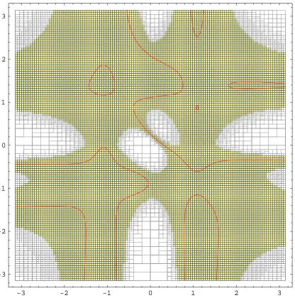
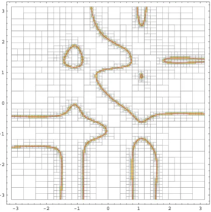
This can be best seen by comparing figure 2.2 and figure 2.3. The result in figure 2.2 is computed using the natural extension and has a quality factor of only 0.0571, much too low to be of any practical use. The result in figure 2.2 is computed using the Midpoint Taylor Form interval extension, see section 3.2.2. It has a much better quality factor of 0.8997.
Although running times are similar, a meaningful comparison of the two approaches could not be made without considering the quality of the interval covering produced. We propose a new measure called the Time/Quality cost:
Time/Quality cost: TQCost Sε= time
Q
Sε.
The Time/Quality cost of the interval covering in figure 2.2 is 1,474.858 seconds, while that of the interval covering in figure 2.3 is 70.038 seconds.
Within this framework one quickly discovers that naive use of natural extensions routinely produces interval coverings of very bad quality, so bad that they are virtually useless. Cases like these are often responsible for the poor reputation interval analysis still has to date. They show how important it is to use inclusion functions with the smallest excess width available.
2.5
Inclusion of the Solution Set of Nonlinear Optimization
Prob-lems
One of the main appeals of interval analysis is its ability to solve very general nonlinear opti-mization problems which would be impossible to solve using most other methods. The basic interval algorithm for optimization is due to Moore and Skelboe and is sketched in figure 2.4.
Like we did in the previous section we first formalize the class of problems we are trying to solve. Let f :Rn→Rmbe a multivariate vector valued function and S be the set of all the global minima of f inside the domain d ⊂Rn:
S={x∈ d | ∀y∈ d,f(x)≤f(x)}.
Once again, we are interested in finding a finite interval covering of S as defined in sec-tion 2.4. Superfluous and proper solusec-tion intervals as well as the quality of an interval covering are defined as before. The same considerations about the relationship between the inclusion function used and the quality of the interval covering and the execution efficiency apply to the Moore-Skelboe algorithm.
2.5.1 The Moore-Skelboe Optimization Algorithm
The pseudocode of the constrained optimization algorithm is shown in figure 2.4. The algorithm maintains a dynamic estimate of the upper bound to the global (constrained or unconstrained) minimum value of the function. The upper bound is used to eliminate regions that cannot contain a global minimum as well as regions that were previously thought to contain a global minimum but eventually become obsolete. This latest process is done by the PurgeObsoleteMinima rou-tine.
For unconstrained minimization the routine SatisfiesConstraints always returns “true”. For constrained minimization problems, the routine returns “true” if there is at least one point inside
x where all constrains are satisfied or “false” otherwise. Writing such a routine for all types of
MooreSkelboeOptimize (
in f: function whose minima we are seeking
in d : domain interval
inε: maximum size of a solution interval
out Sε: [empty] interval covering of the minima of f over d
)
{
create stack: [empty] stack of subintervals to be examined;
real supMin: [∞] current estimate of the upper bound of min
d (f);
put d on stack;
while(stack is not empty)do
{
pop x from stack;
// estimate the range of f on x
compute y =I(f) (x);
if (supMin≥ y )and SatisfiesConstraints( x )
// there could be a global minimum in x
{
// update global minimum
set supMin=min(supMin,y);
// eliminate solution intervals si with inf(I(f) (si))>supMin
PurgeObsoleteMinima in supMin, in/out Sε;
if(w(x)<ε)
append x to Sε;
else
{
Subdivide(in x , out x1, out x2);
put x1on stack;
put x2on stack;
} } }
return; // search is exhausted
[image:43.612.119.531.95.597.2]}
2.6
Inclusion of the Solution Set of Systems of Differential and
In-tegral Equations using Interval Picard Iterations
In this section, we very briefly describe the interval version of Picard’s algorithm for computing Taylor form enclosures for the solution of certain differential and/or integral equations. For more detail refer to [Berz and Hofst¨atter 1998].
Interval Picard iteration is not the only method for solving ODEs using interval analysis. Other methods—such as interval versions of Euler’s method—have been studied.
2.6.1 Definitions
Norm:k f(t)−g(t)k=maxt|f(t)−g(t)|
Lipschitz condition: A function f(t)satisfies a Lipschitz condition on[a,b]if there is a positive
real number L[fa,b]such that for all t1,t2∈[a,b]:
|f(t1)−f(t2)| ≤L[fa,b]|t1−t2|.
Cauchy remainder: If f(t)can be expanded in an Taylor series then there existξt ∈[t0,t]such
that:
f(t) = ∑∞i=0i!1ddtifi(t0)(t−t0)i
= ∑ni=0i!1ddtifi(t0)(t−t0)i+(n+1)!1 d n+1f
dtn+1(ξt)(t−t0)n+1.
The expression:
CR(f,t0,n) =
1 (n+1)!
dn+1f
dtn+1(ξt)(t−t0) n+1,
is called the nthorder Cauchy remainder of f at t0.
Interval Lagrange remainder: ξt is not usually computable in closed form. However, the
following is always true:
ILR(f,t0,n) =(n+1)!1 ddtn+n+11f([t0,t])(t−t0)n+1,
f(t)∈∑n i=01i!
dif
The expression ILR(f,t0,n)is called the nthorder interval Lagrange remainder of f at t0.
2.6.2 Interval Picard Iteration
Consider the following type of differential equation:
y0=F(y).
which can be rewritten in integral form as:
y=y(t0) + Z t
t0
F(y(x))dx.
We further assume that F is a polynomial and therefore Lipschitz everywhere (bounded deriv-ative) and that we can produce an initial polynomial enclosure y∗0 for y over the interval [t0,t0+1/LF], i.e.
y(t)∈y∗0(t),∀t∈[t0,t0+1/LF].
The Picard iteration step
y∗n+1(t) =y(t0) + Z t
t0
F(y∗n(x))dx,
defines successively better polynomial enclosures for y (i.e. it is a contraction around the solution
y of the differential equation). The integration step can be performed symbolically since all
The proof that the above Picard iteration step is a contraction is as follows:
ky∗n+1(t)−y(t)k = maxt|y∗n+1(t)−y(t)|
= maxt
y(t0) +
Rt t0F(y
∗
n(x))dx−y(t0)− Rt
t0F(y(x))dx
= maxt
Rt t0[F(y
∗
n(x))−F(y(x))]dx
≤ maxt Rt
t0|F(y
∗
n(x))−F(y(x))|dx
≤ maxt Rt
t0LF|y
∗
n(x)−y(x)|dx
≤ maxt[(t−t0)LF|y∗n(x)−y(x)|]
≤ (t0+1/LF−t0)LFmaxt|y∗n(x)−y(x)|
= maxt|y∗n(x)−y(x)|
= ky∗n(x)−y(x)k.
If F is not a polynomial, but it can be expanded in a Taylor series then we use the following method. Let Fn∗be the nth degree Taylor series with interval Lagrange remainder of F, i.e.
F(x)∈Fn∗(x) =
n
∑
i=0
1
i! diF
dxi(x0)(x−x0)
i+ILR(F,x0,n).
Then the Picard iteration step is as follows:
y∗n+1(t) =y(t0) + Z t
t0
Fn∗(y∗n(x))dx.
2.6.3 An Example
Let us look at an example of Picard iteration that could be used to solve the differential equation:
y0=y2,y(0) =1
Let y∗0= [1,2]. F(x) =x2and F0(x) =2x. The Lipschitz constant of F on the interval[1,2]is:
Therefore, we can expect a Picard iteration to be a contraction for values of t in the interval [0,1/4]. The first two such Picard iterations are as follows:
y∗1(t) = 1+R0t[1,2]2dx
= 1+ [1,4]t,
y2∗(t) = 1+R0t(1+ [1,2]x)2dx
Chapter 3
Related Previous Work
In this chapter we review some important state of the art interval algorithms. We begin our dis-cussion with a short review of the concepts of Taylor Forms and Taylor Models, see Section 3.1. Next, in Section 3.2 we review the most important methods for the robust inclusion of the range of multivariate functions. Finally, in Section 3.3 we review some of the state of the art Interval Newton methods for the inclusion of the global set of solutions of nonlinear systems of equations.
3.1
Taylor Forms and Taylor Models
We begin our review with a discussion of Taylor Forms because they are the principal tool used to convert nonlinear functions into polynomials, for which all the later methods are developed in the following sections.
Through the following arguments f(x)is a generic real-valued multivariate nonlinear func-tion while p(x)and q(x)are real-valued multivariate polynomials. p(x)and q(x)are interval-valued multivariate polynomials, i.e. they are polynomials with at least one interval coefficient.
Definition 3.1.1 (Taylor Form). An interval-valued polynomial p(x)is a Taylor Form of f(x)
over the interval box d if for∀x∈ d we have:
In other words, a Taylor Form is an interval-valued polynomial that bounds the values of the function f at every point in some given region d . For example, a Taylor Form of cos(x)over the entire real line is:
cos(x)∈1−1 2x
2+ 1
24x
4−[−1,1]
720 x
6.
If all the coefficients of the Taylor Form p(x)are real except for the constant term which is an interval we have a Taylor Model. For example, a Taylor Model of cos(x)over the interval
x∈[−1,1]is:
cos(x)∈
719 720, 721 720 −1 2x
2+ 1
24x
4.
Taylor Models are the sum of a polynomial and an interval called the interval remainder
bound. We write:
f(x)∈p(x) + r,
where r is the interval remainder bound.
Taylor Forms and Taylor Models of analytic functions can be obtained from their Taylor expansions, hence the names. For example, for a one dimensional function f(x)we obtain the
nthTaylor Form over the interval d :
f(x)∈Taylor<n>(f,c) (x) +(x−c)
n+1
(n+1)!
I
dn+1f dxn+1
d
,
where c∈ d andIddxn+n+11f
dis an inclusion function of the n+1st derivative of f evaluated on d . The corresponding Taylor Model can be obtained by replacing the real variable x with the interval d in the(x−c)n+1term:
f(x)∈Taylor<n>(f,c) (x) +(d −c)
n+1
(n+1)!
I
dn+1f dxn+1
d
.
The interval remainder is:
r =(d −c)
n+1
(n+1)!
I
dn+1f dxn+1
d