Analysis of data mining evaluation methods’ efficiency

ORIGINAL RESEARCH ARTICLE

ANALYSIS OF DATA MINING EVALUATION METHODS’ EFFICIENCY

*Roumen Trifonov, Daniela Gotseva and Vasil Angelov

Faculty of Computer Systems and Technology, Technical University, Sofia 1000, Bulgaria

ARTICLE INFO ABSTRACT

After the data mining algorithm has concluded, the results have to be evaluated. The evaluation will show the used algorithm’s accuracy. The main goal of data mining is to discover hidden patterns in data sets. To achieve this there are different algorithms or methods. The algorithms have to be compared based on the work they have performed on the data sets. There are several statistical-based tests to verify that the differences between the methods are not due to some chance effect. Each machine learning technique, used in data mining has different performance in terms of a specific problem. The problem is associated with data set. This article will represent a general overview of the performance measuring techniques.

*Corresponding author

Copyright ©2017,Roumen Trifonovet al. This is an open access article distributed under the Creative Commons Attribution License, which permits unrestricted use, distribution, and reproduction in any medium, provided the original work is properly cited.

INTRODUCTION

The ability to classify accurately test instances is called prediction. There are cases when the prediction is for numeric values and others – for nominal values. Each case requires different methods. If there is a misclassification, this results in error. Depending on the type of the error, there is a different cost for the misclassification. The extracted pattern forms the data set via the data mining process represent a “theory” of the data itself (Witten, 2011). The dataset are separated into several parts. The use of those parts can be for training, testing or evaluation of the learning algorithm. Those parts can be rotated for the use of each particular activity.

Training and testing

The classifier’s performance can be measured in term of error rate. The classifier predicts the class of each instance. If the class is correctly assigned, then there is a success, but if the instance has been classified as incorrect class, there is an error. The error rate is determined by the proportion of errors made over the entire set of instances. The main indicator for the classifier’s accuracy is its future performance on the new data.

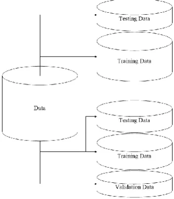
If the old data was used during the learning process used to train the classifier, then the error rate on the old data is not a good indicator for the error rate on the new data. The performance will be optimistic if classifier, learned from the same training data, was used. There is a resubstitution error which is the error rate on the training data. It is calculated by resubstituting the training instances into a classifier that was constructed from them. It is often not reliable (Witten, 2011). There is a need of independent dataset, called test set, used for assessing the error rate, in order to predict the performance of the classifier on new data. The test data must not be used in any way to create the classifier. There are two-staged learning schemes – ones that determine the basic structure and ones used for optimization of the structure’s parameter. All require the data to be partitioned (Figure 1). The training data is used by one or more learning schemes to select the classifier. The validation data is used for optimizing the classifier’s parameters or to select a particular one. The test data is used to calculate the error rate of the final and optimized method. Each of the sets has to be chosen independently – for good performance in the selection and optimization stages and to obtain a reliable estimate of the true error rate. After that the test data may be bundled/returned back into the training data – to produce a new classifier for actual use.

ISSN: 2230-9926

International Journal of Development Research

Vol. 07, Issue, 11, pp.16880-16884, November,2017

Article History:

Received 18th _{August 2017}

Received in revised form 09th September, 2017 Accepted 14th _{October, 2017}

Published online 29th _{November, 2017}

Key Words:

Data mining, Training, Testing, Evaluation, Holdout, Cross-validation, Bootstrap.

Citation: Roumen Trifonov, Daniela Gotseva, Vasil Angelov, 2017. “Analysis of data mining evaluation methods’ efficiency”, International Journal of

Development Research, 7, (11), 16880-16884.

Figure 1. Data partitioning

In that way the amount of data used for generation of the classifier for the practice can be maximized. If large dataset is available, then large sample for training can be combined with another independent large sample for testing. The larger the training sample, the better the classifier. Larger test sample leads to more accurate error estimate. The problem is at hand when there is no vast supply of available data. In the majority of the cases there are limited amount for training, validation and testing. With limited data a certain amount is held for testing – this is the so called holdout procedure. The remainder is used for training and validation if possible. The conclusion is that for a good classifier is needed as much data as possible for training, but for a good error estimate is needed as much from the data as possible for testing (Witten, 2011).

Predicting Performance

The success rate equals the difference from 100 and the error rate. The true success rate is close to the success rate and the larger population in the test set results in true success rate closer to the success rate. The instances in the datasets are independent and succession of independent events that succeed or fail (such as coin tossing) can be described by the Bernoulli process. The observed success rate is:

f = s

N ……..(1)

where p is the unknown true success, s is the success rate and N is the number of trails. The correlation between p and f is described by confidence interval – p lies in a specific interval with a certain specified confidence. The mean value of a single Bernoulli trial with success rate p is p. The variance of a single Bernoulli trial with success rate p is:

p × (1 − p) ………(2)

With N trials that are derived from a Bernoulli trial, the expected success rate is as (1) and the variance is:

× ……….(3)

For large N the distribution of this random variable approaches the normal distribution. For random variable X with zero mean value, the probability lies in the following confidence range of 2z:

Pr[−z ≤ X ≤ z] = C ……….(4)

For normal distribution the values for C and their

corresponding values for z are in tables. The confidence that X will be outside the range is:

Pr [X ≥ z] ………(5)

This is referred as upper tail of the distribution. [3] Due to the symmetric nature of the natural distribution, the probability of the lower tail is:

Pr [X ≤ −z] ………(6)

In the estimation of parameters there is a bias of the used methods. It is defined as the difference between the expected and estimated values. A method with zero bias is unbiased estimation method. But the bias is not a sufficient indicator for the method’s performance. There are cases in which the performance is low, as the bias. But the variance in them is high (Kohavi, 1995).

Holdout method and Cross–validation

Usually there is limited data for training and testing. The aforementioned holdout procedure reserves one amount (usually 1/3) for testing and the remainder (2/3) is for training. Some of the data may be used for validation, if it is required (Figure 2).

Figure 2. Data partitioning for the holdout method

classes’ representation. Bias can be mitigated by repeating the process of training and testing several times with different random samplers. This high variability pays for the bias (Efron, 1997). Each iteration includes a proportion (2/3) of data randomly selected for training (with stratification) and the remainder is for testing. Then the average of all of the iterations’ error rates has to be calculated. This is the so called overall error rate – repeated holdout method of error rate estimation (Efron, 2011). Each test instance in classification is viewed as Bernoulli trial – with correct or incorrect prediction. The holdout estimate is a random number, depending on the dataset’s division in training and test sets. In random sampling, the k-times repetition of the holdout method leads to averaging the results from the runs in order to derive the estimated accuracy (Witten, 2011). Cross – validation includes choosing fixed number of folds (partitions) of data. This is a statistical technique. For example, if there are three numbers of folds available, then the dataset has to be separated into three approximately equal parts (Figure 3). In each turn one partition is used for testing and the remainder is used for training. On a rotating principle 1/3 of the data is used for testing and 2/3 is used for training. There will be three repetitions in total, so that each partition is used for testing one time – threefold cross–validation. If there is stratification – this procedure will be called stratified threefold cross–validation.

Figure 3. Threefold cross-validation

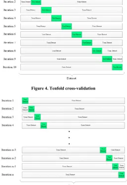
Standard way of error rate prediction of a learning technique with a fixed data sample is the use of stratified tenfold cross-validation (Figure 4). In it the data is separated into ten randomly divided parts (in which each class is approximately represented in the same proportion as in the full dataset). 9/10 parts are for training of the learning scheme. 1/10 part is hold out in each turn. The error rate is calculated on the holdout set. The learning procedure is repeated ten times on different training set (each set has a lot in common with the others). The ten error estimates are used for calculating the overall error estimate (Witten, 2011).

Practice/test and theory show that ten is the best number of folds to get best error estimate. Albeit there is still a debate, ten has been affirmed as a standard in the practice. Tests show that stratification slightly improves the results. The ten folds do not have to be exact. Fivefold or twentyfold cross-validations are also good. They show lower variance, but higher bias for some cases (Efron, 1997) Single tenfold cross-validation might not be enough to produce a reliable error estimate – different tenfold cross-validation experiments with the same learning scheme and dataset often produce different results (due to the effect of random variation in the folds selection). The use of stratification reduces the variation, but does not eliminate it. Standard approach for accuracy for the error estimate is the repetition of the tenfold cross-validation process ten times. After that the result have to be averaged, but

one hundred times invocation/execution of the learning algorithm on datasets with size 9/10 times of the original dataset’s size is computational intensive.

Leave-one-out Cross-validation

This is a type of n-fold cross-validation, where n is the number of instances in the dataset (Figure 5). One instance is left out in each turn. The remaining is used for training the learning scheme. By the correctness on the remaining instances can be judged for the algorithms accuracy – one for success and zero for failure.

Figure 4. Tenfold cross-validation

Figure 5. Leave-one-out cross-validation

each two classes. The best prediction will be with error rate of 50%. But in each fold in leave-one-out, the opposite class to the test instance is in the majority and therefore the predictions will be incorrect, leading to error estimate of 100% (Witten, 2011). This method is reasonable unbiased, but with high variability in some cases (Efron, 1997).

The Bootstrap

This is estimation method, based on the statistical procedure of sampling with replacement. The samples are called bootstrap samples. In the aforementioned methods, when a sample is taken out of a test or training set, it is without a replacement. Once selected, that instance cannot be reselected again. Bootstrap incorporates the idea of sampling the dataset with replacement to form the training set. In its nature, the bootstrap procedure represents a version of the cross-validation methods. (Efron, 1997). This is called 0.632 bootstrap and is the principal example of the bootstrap family algorithms. Dataset of n instances is sampled n timeswith replacement, providing another dataset of n instances. Due to repetition of some instances in the second dataset, some instances in the original dataset have not been picked and they are used as test instances. The probability of picking one instance is 1/n. The probability of not picking instance each time is 1 – 1/n. There are n picking opportunities:

1 − ≈ = 0,368 ……….(7)

This is the chance of a particular instance not being picked at all. For large datasets the test set will contain approximately 36.8% of the instances, meaning that the training set will contain 63.2% of the instances, hence the name 0.632 bootstrap. Some instances will be repeated in the training set and they will bring the total size to n (the size of the original dataset). The training set contains only 63% of the instances, so this will provide a pessimistic estimate of the true error rate, compared to the 90% in the tenfold cross-validation. For compensation the test-set error rate can be combined with the resubstitution error rate on the instances in the training set. The resubstitution figure provides optimistic estimate of the true

error and should not be used as an error figure on its own. But the bootstrap combines it with the test error rate to produce the final estimate is:

e = 0.632 × e + 0.368 × e …(8)

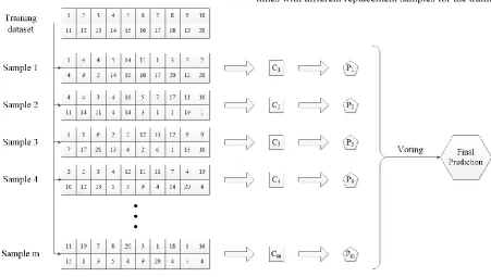
After that the complete bootstrap procedure is repeated several times with different replacement samples for the training set.

Then the results have to be averaged (Figure 6). By selecting n numbers (in the diagram n = 20) of random examples with replacement (equal to the number of elements in the training set) for each one of the m samples, m datasets are produced. Those datasets are used for training m classifiers. Each classifier can be associated with test observation (hypothesis). The observations correspond to predictions. Each prediction is aggregated by voting to a final prediction. The bootstrap procedure is best for small datasets, due to the computing-consuming repetitions (Witten, 2011). Disadvantage is at hand in one artificial case: random dataset with two classes of equal size, meaning 50% true error rate for any prediction rule, but a learning scheme that memorized the training set will provide perfect resubstitution score of 100%. In this case the estimate of the training instances will be equal to 0 and the bootstrap will mix that with a weight of 0.368 to give the following overall estimate:

e=0.632×50%+0.368×0%=31.6% ………(2)

which is misleadingly optimistic (Witten, 2011). The bootstrap method fails in the cases of classifiers with full level of memorization with random datasets (Kohavi, 1995).

Conclusion

While the data volumes are constantly increasing, the use of raw data is inapplicable. Data has to be preprocessed, in order to provide adequate performance for the classification algorithms in the field of data mining. Using statistical approaches, the efficiency of the performance of the algorithms can be determined in a satisfactory degree. The holdout method is the simplest variant of cross-validation. Its low computational time on one side is downsized by the

highly-shifted evaluations. The k-fold cross-validation

improves the holdout method, because the data

division/partition matters to a limited degree. Each data set is used in a test one time and k-1 times for training. Rotating dataset for training and testing reaffirms the algorithms accuracy to a degree with a specific certainty. This method’s disadvantage is that the classification algorithm has to be executed n times, meaning that it will take n times much more computations to produce an evaluation. The bootstrap method is efficient in small volume datasets with low level of memorization classifiers.

REFERENCES

Efron, B. and Tibshirani, R. 1997. Improvements on Cross-Validation: The .632+ Bootstrap Method. Journal of the American Statistical Association, Vol. 92, № 438, pp. 548 – 560.

Kohavi, R. 1995. A Study of Cross-Validation and Bootstrap

for Accuracy Estimation and Model Selection.

International Joint Conference on Artificial Intelligence.

Witten, I., Frank, E., Hall, M. 2011. Data Mining – Practical Machine Learning Tools and Techniques. Third Edition, Morgan Kaufmann Publishers, pp. 147 – 156.