Modelling individual variability in cognitive development

BIROn - Birkbeck Institutional Research Online

Thomas, Michael S.C. and Richardson, Fiona M. and Forrester, Neil A.

and Baughman, Frank D. (2010) Modelling individual variability in cognitive

development. Connection Science , ISSN 0954-0091. (Submitted)

Downloaded from:

Usage Guidelines:

Please refer to usage guidelines at or alternatively

BIROn

-

B

irkbeck

I

nstitutional

R

esearch

On

line

Enabling open access to Birkbeck’s published research output

Modelling individual variability in cognitive development

Journal Article

http://eprints.bbk.ac.uk/2876

Version: Pre-print, submitted

Citation:

© 2010 The Authors

Publisher version available upon publication

______________________________________________________________

All articles available through Birkbeck ePrints are protected by intellectual property law, including copyright law. Any use made of the contents should comply with the relevant law.

______________________________________________________________

Deposit Guide

Contact: [email protected]

Birkbeck ePrints

Birkbeck ePrints

Modelling individual variability in cognitive development

Michael S. C. Thomas

, Fiona M. Richardson

, Neil A. Forrester

, and

Frank D. Baughman

1

Developmental Neurocognition Laboratory, School of Psychology, Birkbeck, University of

London, UK

2

Functional Imaging Laboratory, Institute of Neurology, University College London, UK

Running head: Modelling cognitive variability

Words: 9000 (main text)

Address for correspondence:

Dr. M. S. C. Thomas School of Psychology

Birkbeck College, University of London Malet Street Bloomsbury

Abstract

Investigating variability in reasoning tasks can provide insights into key issues in the study of

cognitive development. These include the mechanisms that underlie developmental transitions,

and the distinction between individual differences and developmental disorders. We explored the

mechanistic basis of variability in two connectionist models of cognitive development, a model

of the Piagetian balance scale task (McClelland, 1989) and a model of the Piagetian conservation

task (Shultz, 1998). For the balance scale task, we began with a simple feed-forward

connectionist model and training patterns based on McClelland (1989). We investigated

computational parameters, problem encodings, and training environments that contributed to

variability in development, both across groups and within individuals. We report on the

parameters that affect the complexity of reasoning and the nature of ‘rule’ transitions exhibited

by networks learning to reason about balance scale problems. For the conservation task, we took

the task structure and problem encoding of Shultz (1998) as our base model. We examined the

computational parameters, problem encodings, and training environments that contributed to

variability in development, in particular examining the parameters that affected the emergence of

abstraction. We relate the findings to existing cognitive theories on the causes of individual

1. Introduction

The computational modelling of cognitive processes offers several advantages. One of the most

notable is theory clarification. Verbally specified theories permit the use of vague, ill-defined

terms that may mask errors of logic or consistency, errors that often become apparent when

formal implementation forces these terms to be clarified. For example, in the domain of

intelligence research, in a verbal theory, one may characterise a more clever cognitive system as

being ‘faster’; but an implemented model of that system must specify what ‘speed’ really means

and how it relates to the quality of computation. In the domain of developmental research, one

may refer to a more developed cognitive system as containing ‘more complexity’; but an

implemented model must specify what ‘complexity’ really means in terms of the structure of

representations and the processes that act on them. In the domain of atypical development, one

may refer to a disordered cognitive system as having ‘insufficient processing resources’; but an

implemented model must specify what a ‘processing resource’ really means, and what

parametric range constitutes an insufficiency with respect to the range found in the typically

developing population.

Connectionist networks have been widely used to model phenomena in cognitive

development because they are essentially learning systems (Thomas & Karmiloff-Smith, 2003;

Thomas & McClelland, 2008). Connectionist models have been applied to a wide range of

developmental phenomena over the last twenty years. These include categorisation and

object-directed behaviour in infants, Piagetian reasoning tasks such as the balance scale problem,

seriation, and conservation, and other children’s reasoning tasks such as learning the relation

between time, distance and velocity, and discrimination shift learning. Within the domain of

categorisation of speech sounds, the segmentation of the speech stream into words, vocabulary

development, the acquisition of inflectional morphology, the acquisition of syntax, and learning

to read (see Elman et al, 1996; Mareschal & Thomas, 2007, for reviews).

Connectionist models embody a range of constraints or parameters that alter their ability

to acquire intelligent behaviours. These include constraints such as the initial architecture of the

network (in terms of the number of processing units and the way they are connected), the

network dynamics (in terms of how activation flows through the network), the way in which the

cognitive domain is encoded within the network (in terms of input and output representations),

the learning algorithm used to change the connection weights or architecture of the network, and

the regime of training the network will undergo. Only the last of these constraints is derived from

the environment; the preceding four are candidates for innate components of the learning system,

although in principle these four constraints may themselves be the products of learning or other

environmental influences on development.

Decisions about the design of the network directly affect the kinds of cognitive problem it

can learn, how quickly and accurately learning will take place, as well as the final level of

performance. To the extent that these networks are valid models of cognitive systems,

differences in these constraints or parameters provide us with candidate explanations for the

variations found both between individuals and within individuals over time. In this paper, we

consider the adequacy of the computational constraints within two established connectionist

models of cognitive development to provide candidate mechanisms for variability in children’s

acquisition of reasoning. The models seek to capture variability in two Piagetian reasoning tasks,

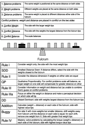
2. Variability in a developmental model of the balance scale task

In the study of cognitive development, a rich literature has accumulated on the balance scale

task. In this task, different numbers of weights are placed at distances either side of a fulcrum

and the child is asked whether the scale will balance, tip left, or tip right when released (Inhelder

& Piaget, 1958). For both empirical and computational approaches to this domain, the

cornerstone is Siegler’s initial work (1976, 1981) in which children’s decisions at different ages

were characterized in terms of four rules of increasing complexity. Rules I to IV describe the

child’s performance on each of the six different problem types (see Figure 1), with Rule IV

representing mastery.

Siegler’s rule assessment methodology has provoked much debate, both with regard to

whether the rules he postulated are sufficient to capture children’s behaviour or are merely

descriptive (e.g., Wilkening & Andersen, 1982) and whether rules actually play a causal role in

driving behaviour (Hardiman, Pollatsek, & Well, 1986). Rule-based theories of development

have traditionally struggled to explain the mechanisms mediating transitions between rule states,

leading to theories based on connectionist learning models (e.g., McClelland, 1989). As an

example of the debate, it has been argued that children use different rules depending on the

torque value (where torque = weight x distance from fulcrum): Ferretti and Butterfield (1986)

found that problems with a large difference in the torque acting on each side were likely to draw

responses consistent with a more advanced rule; Jansen and van der Maas (1997) later reported

that the torque difference effect only occurred for problems with extreme torque values.

===================

Insert Figure 1 about here

Despite criticism, Siegler’s rules have stood the test of time, albeit with proposed

additions (and replacements) to the original four core rules. For example, the smallest distance

down rule (SDD, Figure 1) has been proposed as a rule used by children only when in transition

between rules I and II (Jansen & van der Maas, 2002). The majority of new rules have emerged

through the scrutiny of behaviour surrounding Rule III where, according to Siegler’s scheme,

children perform well when either weight or distance information unambiguously predicts the

side to tip, but then guess when these sources of information conflict. Some of the new rules

proposed to account for the variability around Rule III include: Rule IIIa, the qualitative

proportionality, distance dominant, addition, and buggy rules (Ferretti & Butterfield, 1986;

Jansen & van der Maas, 1997, 2002; Normandeau et al., 1989; van Maanen, Bean & Sijtsma,

1989; Wilkening & Andersen, 1982).

The existence of additional rules has found support from Latent Class Analysis, a

statistical technique for categorizing behavioural data into consistent subgroups (e.g., Jansen &

van der Maas, 1997, 2002). Though these analyses differ in the number of classes generated

(relating to a free parameter in this statistical technique), they converge on the idea that Rule III

behaviour consists of a variety of strategies that children tend to switch between. Recent work

examining reaction times (RT) as well as accuracy has supported the development with age of

more complex balance-scale strategies, favouring the buggy rule over the addition rule as a Rule

III strategy (van der Maas & Jansen, 2003), although the response patterns for buggy and

addition are co-extensive.

Individual variability in performance on different problem types has been acknowledged

in theories of the phases of development. The staircase model captures the phases of

while transitions in the overlapping waves model are more gradual and interleaved, particularly

around Rule III (Siegler, 2002). A combination of these two models (Jansen & van der Maas,

2002) captures the behavioural data via steep transitions between Rule I and Rule II but overlap

and gradual transitions between subsequent rules (such as Rule II, Rule III, and the addition rule)

prior to reaching Rule IV.

Computational approaches have sought to specify the mechanisms that generate the

behavioural profile of development on the balance-scale task. The models are disparate, ranging

from connectionist implementations (Dawson & Zimmerman, 2003; McClelland, 1989; Shultz,

Mareschal & Schmidt, 1994) to production systems (van Rijn, Someren & van der Maas, 2003)

to decision trees (Schmidt & Ling, 1996). Typically, these models have attempted to capture the

sequence of Siegler’s four core rules, and have been judged on their ability to capture the

complete range of behavioural phenomena (van Rijn et al., 2003). However, Dawson and

Zimmerman (2003) have argued that computational modelling has been preoccupied with fitting

the data. Since none of the models give a perfect fit and the detailed data are themselves

contested, at this stage the contribution of models should be a qualitative understanding of the

mechanisms underlying rule transitions (see Quinlan et al., 2007; Shultz & Takane, 2007;

Thomas, McClelland et al., 2009, for recent discussions).

Despite the wealth of research on the balance scale task, one area has remained relatively

under explored until recently. This is the question of variability. The study of variability in

cognitive development is important for three reasons. First, within a single individual, it has been

argued that increased variability in performance presages the onset of developmental transitions

(Jansen & van der Maas, 2002). Second, variability across individuals of the same age gives a

pathway are found in disorders, sometimes exhibiting delay, sometimes failure to reach more

complex levels of reasoning, and sometimes qualitatively atypical patterns. Implemented models

have generally focused on the normative (average) pathway, yet each type of variability must

ultimately be explained at a mechanistic level (Thomas & Karmiloff-Smith, 2003).

The following sections report an initial set of simulation results investigating sources of

variability in the balance scale task. First we introduce our base or ‘normal’ model of

development. Second, we explore how changes to the model’s computational parameters,

representations, and training environment alter its behavioural profile. Third, we evaluate

variability in a single case study.

2.1 The Normal Model

The normal model was defined as a 3-layer feedforward connectionist network consisting of an

input layer of 20 units representing the number of weights placed (up to 5) on each side of the

scale (5 distances either side), a hidden layer of 4 units, and an output layer of 2 units (tip left, tip

right). The model used McClelland’s (1989) input encoding, where weight and distance

information were represented on different units. McClelland’s original model separated channels

for weight and distance processing channels (i.e., a split hidden layer), a design assumption

intended to amplify the model’s difficulty in integrating these dimensions. In contrast, we used

an undifferentiated network because we wished to avoid using a proprietary network architecture

for this particular reasoning problem. There are limitations in our simple model but it remains a

useful launching pad to begin an exploration of developmental variability (see Quinlan et al.,

2007, for criticism of computational models of balance scale; and Schapiro & McClelland, 2009,

The model was trained using back-propagation for 100 epochs, where an epoch is one

presentation of the full training set, and the learning rate was set to 0.01. Ten network runs were

conducted per manipulation, with initial weights randomized between ±0.5. The standard

deviation across runs is depicted in all figures. The training set contained of 621 of the possible

625 balance scale problems for a five-peg scale using up to five weights, and was similar to that

of McClelland in that balance and weight problems were duplication / over-sampled in the

training set. The training set consisting of 1069 patterns. The 24 problems were held back and

used to assess generalization. Performance was measured at 10, 20, 25, 30, 35, 40, 50, 60, 70, 80,

90, and 100 epochs.

The test set consisted of 4 problems from the 6 problem types (see Figure 1). The

model’s performance on the test set was assessed with 7 test metrics. The metrics captured

behavior in line with the following rules: (i) Rule I, (ii) SDD rule, (iii) Rule II, (iv) QP rule, (v)

Rule III, (vi) addition rule, and (vii) Rule IV. Each metric calculated the percentage of responses

consistent with its rule. Note that a given correct response may be consistent with several rules.

For example, Figure 2 shows the problem-space and the proportion of patterns consistent with

the four core rules.

The normal network learned the training set to an accuracy of 98.0% (SD 0.0%). The

mean performance of the normal model on each of the test metrics across training is shown in

Figure 3(a), for the one hidden layer (1HL) condition. Given that we did not separate distance

and weight information in the architecture, the network did not exhibit strong evidence of early

Rule I, SDD, or Rule II behavior, confirming that weight-distance integration difficulties require

architectural assumptions. However, our focus here is upon the model’s balance scale behavior

that best characterized the development of the ‘normal’ model was: QP -> Rule III -> addition

rule -> Rule IV.

====================

Insert Figure 3 about here

====================

2.2 Exploring Variability

Variability was explored by making a series of systematic changes either to the normal model’s

computational parameters, to the problem encoding, or to its environment.

2.2.1 Variability and Computational Parameters

We varied (i) the number of hidden layers, (ii) the number of hidden units in a single layer, and

(iii) the learning rate.

Increasing the number of hidden layers The performance of the model was tested with 2

and 3 hidden layers (HL), with 4 units per layer. Additional hidden layers tend to increase the

computational complexity of the mappings that can be learned by a network, while slowing

down learning since the error signal must filter back through more levels (Beale & Jackson,

1990). So that learning would fall within a 100-epoch window, the learning rate (lr) was

increased as follows: 1HL=0.01, 2HL=0.02, 3HL=0.2 (these values hold for subsequent use of

these architectures unless otherwise stated)1. These networks achieved mean accuracy levels on

the training set of 98.0, 99.8, and 100.0% respectively.The developmental profiles of the

networks are included in Figure 3(a). Increasing the number of hidden layers altered the number

1

These networks showed qualitatively equivalent results to multi-hidden-layer networks trained on the same learning rate with an

of transitions in behavior made prior to approaching Rule IV performance (we define a transition

as a shift in the rule that covers the most behavior, as per Figure 2). The standard deviation

across runs went up as the number of hidden layers increased but notably, phases of development

became less incremental. For example, the sequence of closest fitting metrics for models with

2HL was: QP -> addition rule -> Rule III -> Rule IV, but was just QP -> Rule IV for networks

with 3HL. (This pattern did not result from lr changes, since it did not arise when 1HL was

trained with a learning rate of 0.2). Increasing the power of the network reduced the number of

transitional states it went through in reaching mastery.

Increasing the number of hidden units in a single layerExpanding the number of units in

a single a layer increases the capacity of the network to learn more patterns of a given

complexity (Cybenko, 1989); and allows the network to learn a given problem with smaller

weights, thereby requiring less learning. We evaluated networks with 4, 10, and 20 units in the

hidden layer for the normal 1HL network. After training, all the networks had a mean accuracy

of 98.0%. Their developmental profiles are shown in Figure 3(b). Increasing the number of

hidden units did not change the profiles compared to the normal case. We explored this

manipulation in the 2HL and 3HL networks and found the same result. If the capacity of the

system is measured in parallel processing resources, additional capacity did not alter the

transitional stages through which the system passed but altered the rate at which it did so.

Reducing the learning rateIndividual differences and developmental disorders are

sometimes characterized in terms of delay (Thomas, Annaz, et al., 2009). This term is usually

descriptive, but one obvious way to implement it is to turn down the learning rate. This would

not explain why delay is frequently uneven across problem domains, but we can at least address

Learning rate was reduced in the normal network in four steps as follows: 0.08, 0.06, 0.04, and

0.02. After 100 epochs, these networks achieved mean accuracies 98.0, 97.1, 94.1, and 56.7%

respectively. Slower learning rates caused roughly parallel shifts for all metrics so that

characteristic patterns in the developmental profiles appeared after more epochs of training.

While development slowed down, the order of the transitions between types of reasoning

behaviour remained the same. When the learning rate was insufficient to achieve mastery within

the fixed time window of 100 epochs, performance terminated at a less complex level. For

example, networks with a learning rate of 0.04 had reached Rule III but not IV, by 100 epochs,

and networks with a learning rate of 0.02 had reached the addition rule. However, were training

extended, Rule IV would be reached in both cases. By contrast, developmental disorders typically

exhibit asymptoting performance at less complex levels of reasoning (Thomas, Annaz et al.,

2009). For individual differences, it is unclear whether everyone eventually ‘catches up’.

Reduced learning rate does not, therefore, seem a good (sole) candidate to explain the type of

developmental delay found in disorders.

2.2.2 Variability and the Problem Encoding

We explored two variations in the problem encoding. These correspond to alterations in the way

in which the problem is presented to the child (perhaps in the salience of different information or

options) or to alterations in how the problem is encoded in the part of the cognitive system

required to predict outcomes of balance-scale problems. We either: (i) added a further response

option so that the scale could either tip left, tip right, or balance; or (ii) altered the input coding

so that information about the weights was represented with position-specific units.

Changing the response options In the normal model, there were two output units whose

by more than 0.33, the response was ‘tip left’, and vice versa for ‘tip right’. If the difference

between the units was less than 0.33, the response was taken to be ‘balance’ (McClelland, 1989).

However, since balance is a legitimate response for a proportion of the problems, it could

reasonably be encoded as a separate output unit. For this condition, a response was considered

correct if the activation of the corresponding output unit was >=0.5 and the activation of any

other output unit was <0.5. Finally, because encoding of the problem domain could alter its

complexity, we contrasted performance on 1HL, 2HL, and 3HL networks with 4 hidden units per

layer. After training, these networks achieved mean accuracy levels of 86.3, 87.5, and 99.2%,

respectively. The developmental phases are shown in Figure 4(a). Comparison with Figure 3(a)

reveals that the additional response option dramatically changed the pattern of transitions. 1HL

and 2HL networks began in Rule I and did not exceed Rule II. Only the 3HL network reached

Rule IV. Changing the response options altered the categorization that the internal

representations had to make across problem types. It ramped up the complexity of the task, since

balance had to be computed internally rather than left to the competition between left and right

output units. More computational power was therefore required for successful acquisition, under

this encoding.

Combined Weight-Distance Encoding In McClelland’s (1989) formulation, weight and

distance information were encoded separately. However, one could represent the number of

weights on each peg locally at each distance. For this manipulation, there were 10 input units,

one for each peg on the balance scale. The activation level coded the number of weights placed

on a peg. Activation ranged from 0 to 1 and each weight was represented by an increment of 0.2.

Thus, three weights on a peg corresponded to an activation of 0.6. The composition of the

3 hidden layers were run to assess the demands of this encoding. The results are in Figure 4(b).

The final performance of the models was poorer than with the normal encoding by around 20%

(1HL=80.2%, 2HL=65.0%, 3HL=90.3%). As above, only the 3HL network achieved Rule IV

reasoning as the closest fitting metric at the end of training. 1HL only reached the QP rule.

Again, a recoding of the problem domain, this time at input, increased the complexity of the task

and altered the developmental phases exhibited by the model.

==================

Insert 4 about here

==================

2.2.3 Variability and the Engaged Environment

Since development in the balance scale task corresponds to the child’s active exploration of the

domain, we refer to the training set as the engaged environment. We created two variations in the

environment: (i) an impoverished training set with restricted coverage of the problem space, and

(ii) a training set without a bias to increase the salience of the weight dimension. In these cases,

the normal architecture and problem encoding was used. 1HL, 2HL, and 3HL networks with 4

units per layer were also contrasted to explore whether additional representational power could

overcome limitations in the engaged environment.

An Impoverished Engaged EnvironmentThis engaged environment consisted of a subset

of 703 training patterns, which excluded any problems where the distances from the fulcrum on

either side was >=3. After training, the 1HL, 2HL, and 3HL reached accuracy levels of 97.8,

99.7, and 100.0%, respectively. This environment had an adverse effect on the single hidden

layer network, where the closest fitting metric at the end of training was Rule III instead of the

fewer transitions. In contrast, for 2HL and 3HL networks, the closest fitting test metric at the end

of training was still Rule IV, with the 2HL network making more transitions than the 3HL. For all

models, there was a considerable increase in variability between individual runs compared to the

normal environment. This impoverished environment, then, increased developmental variability

between individuals. Importantly, with respect to the generalization set at least, the impoverished

environment could be compensated for via a more powerful learning system.

An Unbiased Engaged EnvironmentThe unbiased engaged environment consisted of

1069 patterns where the original bias for the weight dimension was removed. The duplicated

weight problems were replaced with a random selection of patterns already in the training set.

All models trained using this environment were able to reach Rule IV performance. However,

this environment reduced the number of transitions between rules across training.

2.2.4 Individual Variability: A Case Study

Variability also occurs during the development of individual children, including regression to

less sophisticated rules. However, averaging across individuals’ risks producing variability not

found in any one, which may be the case for simulations as well. In this section, we report the

rule transitions in the trajectory of a single network (1HL, lr=0.008, normal encoding and

training set). Performance on the training set is shown in Figure 5(a), while 5(b) illustrates

performance on the 6 problem types in the generalization set at 25, 40, 60, 70, and 100 epochs.

Figure 5(c) depicts the rule transitions shown by this individual network. The model made the

following transitions: QP -> addition -> Rule III -> addition -> Rule IV. The trajectory confirms

variability around Rule III, with a jump from QP to addition, back to the less sophisticated Rule

Inspection of Figure 5(b) suggests that this variability was driven by the network’s

attempts to solve the low-salience distance problems. Performance on balance and weight

problems was robust from early on, but the network struggled to accommodate distance and

conflict-distance problems, inducing greater variability and more transitions between 60 and 80

epochs. In sum, the variability found in averaged data was not an artifact of averaging but found

in individual runs. Apparent rule transitions, including regressions, were a key feature of the

network’s attempts to integrate weight and distance information in solving balance scale

problems.

=====================

Insert 5 about here

=====================

2.3 Summary of Balance Scale findings

Simulation of the balance scale task indicated that variations of internal computational

parameters, problem encoding, and engaged environment all acted on the complexity of the

reasoning exhibited by the network during learning, including the findings that more hidden

layers increased complexity but not more units per layer (contrasting reasoning power with

plasticity); that a slower learning rate did not reduce complexity per se, and is therefore a poor

model of unresolved developmental delay; and that an impoverished environment reduced

complexity but could be compensated for (in terms of generalization performance) by a more

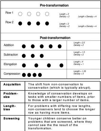
3. The Conservation task

Conservationrefers to the understanding or belief in the continued equivalence of two physical

sets following a transformation that appears to alter one and not the other. A given

transformation may alter a quantity, e.g., by adding or subtracting, or preserve it, e.g., through

elongation or compression. The acquisition of conservation knowledge involves learning to

distinguish between transformations that preserve and those that alter a quantity. For example, in

a typical number conservation task, as shown in Figure 6, a child is initially presented with two

rows of counters (pre-transformation). The child is then asked whether these rows have the same

number of counters or whether one has more than the other. A transformation is then applied to

one row, and the child is asked again whether the two rows are the same, or whether one now has

more counters than the other (post-transformation).

======================

Insert Figure 6 about here

======================

Piaget (1965) found that young children below 6-7 years are non-conservers, in that when

presented with a transformation that preserves number (such as elongation or compression) they

answer that one row has more counters than the other. In contrast children older than 6-7 years

are conservers, having learnt that transformations of this type do not alter number. This finding

has been corroborated across a range of conservation tasks, such as mass (using modelling clay),

liquid quantity (using beakers), and number (using counters) (Brainerd & Brainerd, 1972;

Halford & Boyle, 1985; Klah, 1984; Miller & Heldmeyer, 1975; Siegler, 1995; Siegler &

Robinson, 1982; Wallach, Wall & Anderson, 1967; Winer, 1974). The shift to conserving may

the same, even when their observed perceptual properties have altered. The rich literature on

conservation has also established a series of biases that occur as young children learn to

conserve, relating to problem size, length, and mode of presentation. These effects are

summarized in Figure 6.

While a range of classic Piagetian reasoning tasks such as conservation, seriation and the

balance scale, have been subject to computational investigation, Shultz and colleagues have

argued that a key implementational feature may be necessary for learning systems to exhibit

qualitative changes in the complexity of reasoning (Shultz, 1998; Schultz, Mareschal & Schmidt,

1994). In constructivist networks, networks change their architecture as a function of learning.

One example of an algorithm that implements this approach is cascade-correlation (Falham &

Lebiere, 1990). During training, network connections are altered but if learning stagnates, the

size of the hidden layer is increased. Specifically, connections to existing hidden units are frozen,

and a new hidden unit it added. The hidden unit is connected to the input layer and also to all

existing hidden units, thereby allowing the additional internal resources to make use of the

representations that have already been developed. This allows networks to be constructed which

have representational depth (in the sense of multiple hidden layers) rather than just breadth (in

the sense of more units in a single layer).

Shultz (1998) used such a constructivist network to model development on the

conservation task. He ascribed the ability of his model to capture the abrupt shift from

non-conservation (NC) to conservation (C) to addition of hidden units and an attendant increase in

representational power. However, it is possible that other computational parameters have a

similar impact upon a model’s behavioural profile over the course of development. In the

task as our starting point. We once again introduce a normal, base model of development, and

then proceed to explore how manipulating the model’s computational parameters, input

encoding, and training environment alter its developmental behavioural profile.

3.1 The Normal Model

The base model set out to simulate the development of number conservation, as depicted in

Figure 6. The normal model was defined as a 3-layer feedforward connectionist network

consisting of an input layer of 13units, a hidden layer of 4 units, and an output layer of 2 units.

The problem encoding used by this network was based on Shultz (1998) and is shown in Figure

7. Each row of counters was represented over 2 units, encoding row length and density

respectively, as continuously valued activation levels. Both rows are shown represented in their

pre- and post-transformation states. The row transformed (either row 1 or row 2) was indicated

by the activation (-1 or +1) of a single unit.2 The transformation type was encoded arbitrarily

over 4 units, with the activation of a single unit indicating the type as follows: addition (1 1 1

-1), subtraction (-1 1 -1 -1), elongation (-1 -1 1 -1), or compression (-1 -1 -1 1). The three

possible response options were encoded over 2 binary output units as follows: (i) row 1 longer (1

0), (ii) row 2 longer (0 1), (iii) both rows equal (0 0). The base model differed from Shultz

(1998) in that we employed a standard feedforward architecture with a sigmoid rather than

hyper-tangent activation function.

====================

Insert Figure 7 about here

====================

2

The model was trained using back-propagation for 1500 epochs, with a learning rate of

0.025. Ten network runs were conducted per manipulation, with initial weights randomized

between ±0.5. The standard deviation across runs is depicted in all figures. The composition of

the training and test sets was drawn from Shultz (1998), with patterns having five levels of row

length and five levels of density. A total of 400 training patterns and 100 test patterns were

selected from a full set of 600 possible conservation problems (based upon 25 initial rows, 3

possible start states, and 4 possible transformations for each of the 2 rows). Performance was

assessed at 5, 25, 50, 100, and 200 epochs, and then at every subsequent 100-epoch interval until

the end of training at 1500 epochs.

In order to assess the behavior of the model, the test set was used in conjunction with 4

metrics, each reflecting a target behavioral phenomenon described in Figure 6: (1) the profile of

Acquisition, (2)the Problem Size Effect, (3) the Length Bias Effect, and (4) the Screening Effect.

Metric 1 plotted the development of knowledge of conservation, and calculated the percentage of

test patterns correct. Metric 2 calculated the proportion of small vs. large problem types correct.

In this case, the test set consisted of 40 patterns, 20 small problem types (<12 items), and 20

large (>24 items). Metric 3 used elongation and compression problems from the test set (a total

of 18 patterns, 8 and 10 of each type respectively) to calculate the proportion of patterns where

the longer row was selected as having more items than the shorter row. Metric 4 calculated the

proportion of unscreened vs. screened problems correct for the complete test set. Test patterns

presented to the network were represented as “screened” by replacing post-transformation

activation values with zeros.

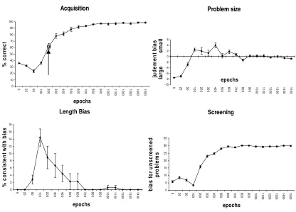
The base network learned the training set to an accuracy of 99.5%. Training performance

patterns correct). The emergence of abstract knowledge was marked by the network’s ability to

discriminate transformations that altered the (abstract property of) number from those that did

not. This shift was preceded by an initial decline in training performance over the first 50 epochs

and followed by small incremental improvements in performance as training progressed. The

behavioral profile of the model can be seen in Figure 8, where the shift from NC=>C

(Acquisition) on novel patterns occurs between 100-200 epochs and performance leaps from

36.2% to 61.7%. The normal profile represents a non-linear shift to conserving. The model also

exhibited a minor performance advantage for small problem sizes (Problem Size effect) between

100-700 epochs, the time during which the model was doing the bulk of its learning. Normality

is defined as an advantage for small problems (+ve values on the chart) during earlier phases of

training. The model’s bias for selecting longer rows as having more items (Length bias effect)

was also found to reduce after this point in learning. Normality is defined as an early positive

spike on the length bias chart. Unlike Shultz (1998), our model did not show any preference for

“screened” problems early in learning (Screening effect), which would appear as an early

negative spike on the chart. This shortcoming may relate to our use of sigmoid processing units

(see later). Nevertheless, in contrast to Shultz (1998), the model was able to show a shift from

non-conserving to conserving within a fixed architecture.

======================

Insert Figure 8 about here

======================

3.2 Exploring Variability

With our base model in hand, we then sought to assess the influence of several factors on

development. Variability was explored by systematic changes to (1) the base model’s

computational parameters, (2) its problem encoding, or (3) the training environment.

3.2.1 Variability and Computational Parameters

The computational parameters that were varied included: (i) the number of hidden layers, (ii) the

number of hidden units in a single layer, (iii) the learning rate, and (iv) the slope of the sigmoid

transfer function for hidden layer units.

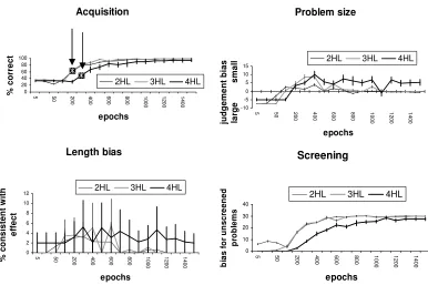
Increasing the number of hidden layers The performance of the model was tested over

learning with 2 and 3 hidden layers (HL), with 4 units per layer. So that learning would fall

within a 1500-epoch window, the learning rate (lr) was increased as follows: 1HL=0.025,

2HL=0.05, 3HL=0.075 (these values hold for subsequent use of these architectures unless

otherwise stated). These networks achieved mean accuracy levels on the training set of 99.5,

99.9, and 99.7%, respectively. The developmental trajectories of the networks are shown in

Figure 9. The profiles of networks with 1HL and 2HL were very similar. Both 1HL and 2HL

networks showed a shift from NC => C between 100-200 epochs. The shift was slightly larger

for networks with 1HL than those with 2HL (26.5 and 35.5%, respectively). Networks with 3HL

showed a smaller initial shift (19.0%), occurring later between 200-300 epochs, followed by a

second successive shift (17.4%) occurring between 300-400 epochs. There was a sustained effect

of Problem size for networks with 3HL, as well as an increase in variability. The variability for

the Length bias effect was very high, particularly for 2HL and 3HL networks. As for Screening,

there was no bias in early learning for screened problems, contrasting with the empirical data.

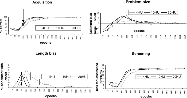
Increasing the number of hidden units in a single layer We assessed networks with 4, 10,

and 20 units in the hidden layer (HU) for the normal 1HL model. At the end of training networks

with 4HU had a mean accuracy of 99.5%; 10HU and 20HU networks had reached 100%. 10HU

and 20HU networks showed earlier Acquisition of conservation knowledge (between 50 and 100

epochs). This shift was also larger than networks with 4HU (30.3% in comparison to 25.5%).

The behavioural profile across metrics can be seen in Figure 10. All networks showed a similar

profile across testing metrics. Variability was uniformly low across metrics. Interestingly,

networks with 4HU did show a slightly larger Length Bias effect of an extended duration, in

comparison to 10HU and 20HU networks. This suggests that the smaller representational space

compromised the network’s ability to drive differential output responses when the net input

activations were low. In broad terms, however, expanding the capacity of the system in terms of

parallel processing resources altered the onset of learning, but not the overall developmental

profile, as observed for the balance-scale simulations.

==========================

Insert Figure 9 and 10 about here

==========================

Reducing the learning rate To address the issue of delay, the learning rate was reduced in

the normal network in four decrements from 0.025 to 0.02, 0.015, 0.01, and 0.005. After 1500

epochs, these networks achieved mean accuracies 99.8, 98.5, 96.6, and 86.3%, respectively.

Lower learning rates slowed down development. As a result, improvements in performance

behaviour were more incremental. This was reflected in the gradual decline in the size of the

shift from NC=>C with decreasing learning rate (from 25.4% for 0.02 to 7.7% for 0.005).

Though networks with a lower learning rate had a lower level of performance at end of training

(at 1500 epochs), performance was steadily increasing, and could have improved further were

training time to be extended. There was no indication of a lowering in the maximum

performance level simply by virtue of a reduced learning rate. As with the balance-scale

simulations, a reduced learning rate does not seem a good (sole) candidate to explain the type of

developmental delay found in disorders with learning disability, where reasoning ability

frequently asymptotes at a lower level.

Decreasing the sigmoid slope Since we had altered the activation function of the

processing units from the original Shultz (1998) of conservation, we investigated the impact of

this function on development. The function determines the activation level of hidden and output

units, given the net input activation they are receiving. Shultz (1998) used a hyper-tangent

function, while we employed a more standard sigmoid function. We explored the impact of the

slope of the sigmoid, which changes how much a processing unit can alter its activation level for

a given change in the net input it is receiving. This in turn impacts on the nature of the category

distinctions a unit can make. For example, a steep sigmoid slope results in sharp category

boundaries and is good for tasks where the model is required to make rule-like distinctions,

whereas a shallow slope is better suited to fine-grained distinctions and tasks with broad category

boundaries. Altering the level of processing unit discriminability has been shown to produce

patterns of deficits consistent with those seen in developmental disorders (Thomas, 2005;

Thomas & Karmiloff-Smith, 2003). For all processing units, the slope of the sigmoid function

was reduced (from a value of 1) in the normal model, by four levels of decreasing

discriminability as follows: 0.8, 0.6, and 0.25, to 0.125. Changing the slope of the sigmoid had a

exhibited a shift from NC=>C, resulting in low mean accuracies at the end of training at all

levels, as follows: 34.5, 34.0, 38.4, and 28.3%, for the 4 decrements respectively. Performance

that was uniformly low for all test metrics. This could not be overcome through the addition of

extra hidden layers, suggesting that the model requires processing units with a high level of

discriminability in order to achieve task success. This is because conservation requires the

network to ignore certain differences in the input. To do so requires a non-linear response. A

shallower sigmoid provides the network with a more linear system, more suited to providing

proportional responses to proportional changes in the input. However, a screening effect (see

Figure 6) appeared for the shallowest slope, suggesting that this developmental phenomenon

may relate to the nature of the non-linear activation function used in the network’s processing

units.

3.2.2 Variability and the Problem Encoding

We explored a variation in problem encoding where the salience of transition type was increased.

It is this information that drives the emergence of ‘abstraction’. The number of units encoding

transition information (as shown in Figure 7) was doubled from 4 to 8, thereby increasing the net

activation arriving at the hidden layers from this information. The architecture now included an

input layer consisting of 17 units, with 8 units encoding pre- and post-transformation

information, and 8 units encoding transformation type. This manipulation was carried out for

networks with 1HL, 2HL and 3HL. The final performance of the models was found to be similar

to that shown for equivalent models trained without increased transition information. The overall

equivalent models. Therefore, for these simulations, changing the salience of a dimension of

information did not have any notable impact upon the developmental trajectory of the model.

3.2.3 Variability and the Engaged Environment

We manipulated the engaged environment, corresponding to the child’s active exploration of the

domain, by creating a training set with a limited coverage of the problem space of the

conservation task.It consisted of 400 problems with a small quantity of items only (<12 items).

The base architecture and problem encoding were used. Networks with 1HL, 2HL and 3HL were

trained on this environment to explore any interaction between representational power and the

engaged environment. Interestingly, this environment did not appear to have notable impact upon

the overall performance, irrespective of the number of hidden layers in the model. At the end of

training 1HL, 2HL and 3HL networks reached the mean accuracies of 99.8, 99.4, and 97.3%,

respectively. The profile of 1HL and 2HL networks over metrics was similar to that shown for

equivalent models trained on a normal engaged environment. Limiting the engaged environment

to problems with a small number of items did not in this case impact upon the developmental

trajectory of the model.

3.2.4 Individual Variability: A Case Comparison

Once more, to distinguish individual profiles from group averaged data, we compared two

individual cases. These were: (i) a single normal model with 1HL (henceforth the Normal case),

and (ii) a 1HL model with a reduced learning rate (lr=0.005, henceforth Reduced lr case). Both

models were trained using the normal input encoding and engaged environment using the same

randomly initialized starting weights. The behavioral profile of each model was assessed using

transformation type, and (ii) problem size was conducted for test items. As expected, the profile

of the Reduced lr network exhibited a slower developing, more incremental trajectory. The shift

from NC=>C was markedly later than in the normal case, by approximately 500 epochs.

Subsequent improvements in training performance were also smaller.

======================

Insert Figure 11 about here

======================

This pattern in training performance is also reflected behavioral profile for the metric

Acquisition (calculated on novel test items) shown in Figure 11. For the next two metrics, the

Reduced lr case showed extended Problem Size and Length Bias effects. These paralleled the

protracted learning window of this model. For the Screening metric, the trajectory of the

Reduced lr case deviated from that of the normal case, demonstrating a minor preference for

“screened” problems at the onset of acquisition of conservation knowledge. An examination of

the development of conservation knowledge in the normal case across problem types (as shown

in Figure 12a) revealed a difference in initial profile for problems that alter number (addition and

subtraction) in comparison to those that preserve number (elongation and compression).

Addition and subtraction problems showed a static level of performance early in learning,

whereas elongation and compression problems showed an initial dip in performance. As a

consequence, performance over learning on transformations that preserved number was poorer

than those that altered it. This dip was seen on all problem types in the lr case. An initial dip in

performance can also be seen for problems of differing sizes (Figure 12b). In the normal, case

this dip was exaggerated for large problem sizes, resulting in poorer performance on large

performance for larger problem types was superior. The atypical case, therefore, exaggerated an

early dip in performance and a reliance on large problem sizes in solving conservation problems.

=======================

Insert Figure 12 about here

=======================

3.3 Summary of Conservation findings

A fixed architecture network demonstrated the ability to learn to conserve abstract properties

across transformations, within Shultz’s (1998) formulation of this Piagetian problem domain. In

some cases, changes to the internal computational parameters of the model had a marked impact

upon the acquisition of conservation knowledge. Once again, changes in serial resources (hidden

layers) altered the profile of development, while changes in parallel resources (within a layer)

altered the rate of development. Changes to the internal discriminability of processing units via

the slope of the sigmoid activation function resulted in a failure to conserve. Decreasing the

learning rate resulted in only a slower rate of acquisition. By contrast, for this model, changes to

the problem encoding at input or the engaged environment had little impact on the model’s

developmental trajectory.

4. Discussion

The advantage of implementation is that it forces theory clarification, while the disadvantage is

that models necessarily involve simplification. In this case, we sought to explore the mechanistic

basis of individual variability via parametric variations to established models of the development

of reasoning in two Piagetian tasks: balance scale and conservation. The former involves

whether a scale will balance. The latter involves learning that certain transformations do not alter

an abstract property (such as number) while others do. In both cases, the base models simulated

the development of these abilities via supervised learning and exposure to many examples of

these problems (McClelland, 1989; Shultz, 1998). Clearly, these reasoning domains are fairly

simple, and far from capturing the full range of skills which developing children exhibit.

Nevertheless, both normal models are targeted at tasks of key theoretical interest within a

Piagetian framework of the development of abstract reasoning abilities.

Our interest here was to address the mechanisms that explain how children of the same

age can differ in their reasoning abilities, in a framework that captures the improvement of these

abilities across development. A number of theoretical proposals have been put forward to explain

the respective mechanisms of individual differences and cognitive development, either at the

cognitive or brain level. For example, with respect to individual differences, several authors have

proposed that differences in cognitive abilities between children of the same age can be

explained by differences in the speed of processing among basic cognitive components, on the

grounds that speed of response in simple cognitive tasks predicts performance on complex

reasoning tasks; and at a brain level, that neurophysiological measures such as latency of average

evoked potentials and speed of neural conductivity correlate with IQ (Anderson, 1992, 1999;

Eysenck, 1986; Jensen, 1985; Nettelbeck, 1987). Sternberg (1983) proposed differences in the

ability to control and co-ordinate the basic processing mechanisms, rather than in the functioning

of the basic components themselves. Finally, Dempster (1991) proposed differences in the ability

to inhibit irrelevant information in lower cognitive processes, since individuals can show large

With respect to mechanisms that might underlie cognitive development, we once more

find speed of processing offered as a factor that may drive improvements in reasoning ability

(Case, 1985; Hale, 1990; Kail, 1991). Case (1985) suggested that an increase in speed of

processing aids development via an effective increasing in short-term storage space, allowing

more complex concepts to be represented. Halford (1999) proposed that the construction of

representations of higher dimensionality or greater complexity is driven by an increase in

processing capacity where processing capacity is a measure of the ‘cognitive resources’ allocated

to a task. Lastly, Bjorklund and Harnishfeger (1990) proposed improvements in the ability to

inhibit irrelevant information, based on evidence from cognitive tasks and changes in the brain

that might reduce cross-talk in neural processing, such as the myelination of neural fibres and the

decrease with age in neuronal and synaptic density.

Here, we considered three types of manipulation that might influence the development of

reasoning ability, within the framework of implemented connectionist models. These were the

computational parameters of the learning system, the encoding of the problem domain, and the

training set to which the network was exposed (corresponding to the model’s engaged

environment). Respectively, the first of these manipulations influences the representational states

that the learning system is able to acquire, the second influences the complexity of the mapping

problem that must be learned, and the third influences the data available to search the

representational states of the system. We contrasted results from simulated development in two

separate reasoning domains, in order to distinguish patterns emerging from the structure of those

domains from those arising from our computational manipulations. In addition, we avoided

domain-specific architectural assumptions to focus on the influence of more domain-general

number of layers, the nature of the activation function, and so forth. Our results revealed the

following pattern.

First, increasing the number of hidden unit layers altered the complexity of the reasoning

behaviour that a network could acquire, but it did so at the expense of slowing down the rate of

acquisition. By contrast, increasing the number of units within a layer did not alter the

complexity of the behaviour acquired (in terms of the domain-specific performance metrics) but

increased the rate at which they were acquired. Changes in serial versus parallel representational

resources therefore appeared to have contrasting effects.

Changes in the learning rate did not alter the quality of developmental profiles, simply

requiring the network to gain greater exposure to the problem domain to reach a given level of

performance. Learning rate has been put forward as a neurocomputational parameter (in the

guise of ‘neuroplasticity’) that might explain general intelligence (Garlick, 2002). Our current

findings suggest that if this were the case, the less intelligent should catch up with the more

intelligent if they are simply given more time to gain relevant experience. There is some

evidence that this prediction holds in childhood, through the use of experimental designs where

children of disparate chronological age are matched at a given mental age (e.g., a younger high

ability group is matched on mental age to an older low ability group). However, this work also

suggests subtle differences between performance achieved via greater intelligence versus that

achieved via greater chronological age (Baughman, 2009). Moreover, as the comparison is

extended into adulthood, the prediction starts to diverge with the prediction. It becomes clearer

that differences in intelligence produce asymptotes in development to different levels in

functioning. This pattern is particularly apparent in individuals who have developmental

lower level (Thomas, Annaz et al., 2009). Learning rate, therefore, may have limitations as a

candidate explanation of individual differences in development. Changes in serial resources

appear to offer more promise, as these clearly altered the level at which reasoning performance

asymptoted.

The modelling results pointed to other factors that could alter the profile of development

in Piagetian reasoning tasks. These included changes to the composition of the training set,

changes to the encoding of the problem domain, and changes to the activation function of

processing units. In the first of these cases, the impact appeared more domain-specific. For the

manipulation we considered (i.e., restricting the training examples to problems specified over a

small values), the balance-scale model was more affected than the conservation model.

Moreover, as least with respect to extracting the general function of this domain (tested on the

novel problem set), some parameters within the balance-scale model demonstrated compensation

for restrictions in the nature of the training set. Lastly, since unit activation functions are argued

to be modulated by attention which itself varies between children (Cohen, Dunbar, &

McClelland, 1990) and since the encoding of problems may differ in more and less intelligent

children (Spitz, 1982), these manipulations provide further avenues for explaining individual

differences in development.

The current work only points in a direction of advancing our understanding of theories of

development and individual differences, via exploring the parameter space of implemented

computational models. Paradoxes still remain. For example, as we have seen, cognition in more

intelligent individuals is linked to greater processing speed, and at the same time, the utilisation

of more complex (perhaps more abstract) representational states. However, as both simulations

were slower, not faster to develop. In machine learning terms, such systems possess a richer

hypothesis space, and this space takes longer to search given the data in the training set. In order

to link greater representational complexity with greater processing speed and faster learning,

more detailed models will be required. In particular, it is likely that we will have to utilise

attractor networks with activation dynamics that exhibit settling into stable representational

states in order to drive responses. This will permit investigations of the relationship between the

rate of settling and the parameters that allow more complex representational states to be

acquired. Moreover, there are a host of more complex reasoning domains to which models must

be applied for a fuller picture of the development of reasoning.

We would argue, in sum, that our understanding of variation in cognition has much to

Acknowledgements: This research was supported by UK MRC CE Grant G0300188 to Michael

References

Anderson, M. (1992). Intelligence and development: A cognitive theory. Oxford: Blackwell.

Anderson, M. (1999). The development of intelligence. Hove: Psychology Press.

Bjorklund, D. F. & Harnishfeger, K. K. (1990). The resources construct in cognitive

development: Diverse sources of evidence and a theory of inefficient inhibition.

Developmental Review, 10, 48-71.

Case, R. (1985). Intellectual development: Birth to adulthood. Orlando, FL: Academic Press.

Cohen, J., Dunbar, K., & McClelland, J. (1990). On the control of automatic processes: A

parallel distributed processing model of the Stroop effect. Psychological Review, 97,

332-361.

Baughman, F. D. (2009). Is intelligence like having a little more cognitive development?

Empirical and computational investigations of the relationship between two forms of

cognitive variability in typically developing children. Unpublished Doctoral Thesis.

University of London, UK.

Beale, R., & Jackson, T. (1990). Neural computing. Bristol, UK: Adam Hilger.

Brainerd, C.J. & Brainerd, S.H. (1972). Order of acquisition of number and quantity in

conservation. Child Development, 43(4), 1401-1406.

Cybenko, G. (1989). Approximation by superpositions of a sigmoidal function. Math. Control,

Signals, Syst., 2, 303-314.

Dawson, M. R. W., & Zimmerman, C. (2003). Interpreting the internal structure of a

connectionist model of the balance scale task. Brain and Mind, 4, 129-149.

Dempster, F. N. (1991). Inhibitory processes: A neglected dimension of intelligence.

Eysenck, H. (1986). The theory of intelligence and the psychophysiology of cognition, (pp. 1-

34) in R. J. Sternberg & D. K. Detterman (Eds.), What is intelligence: Contemporary

viewpoints on its nature and definition. Norwood, NJ: Ablex.

Fahlman, S.E., & Lebiere, C. (1990). The cascade-correlation learning architecture. In D.S.

Touretzky (Ed.), Advances in neural information processing systems 2 (pp. 524-532). Los

Altos, CA: Morgan Kaufmann.

Ferretti, R. P., & Butterfield, E. C. (1986). Are children’s rule-assessment classifications

invariant across instances of problem types? Child Development, 57, 1419-1428.

Garlick, D. (2002). Understanding the nature of the general factor of intelligence: The role of

individual differences in plasticity as an explanatory mechanism. Psychological

Review, 109(1), 116-136.

Hale, S. (1990). A global developmental trend in cognitive processing speed. Child

Development, 61, 653-663.

Halford, G. (1999). The development of intelligence includes the capacity to process relations of

greater complexity, (pp. 193-214) in M. Anderson (1999).

Halford, G. S., Andrews, G., Dalton, C., Boag, C., & Zielinski, T. (2002). Young children’s

performance on the balance scale: The influence of relational complexity. Journal of

Experimental Child Psychology, 81, 417-445.

Halford, G. S., & Boyle, F.M. (1985). Do young children understand conservation of number?

Child Development, 56 (1), 165-176.

Hardiman, P. T., Pollatsek, A., & Well, A. D. (1986). Learning to understand the balance beam.

Hertz, J., Krough, A., & Palmer, R.G. (1991). Introduction to the theory of neural computation.

Reading, MA: Addison-Wesley.

Inhelder, B., & Piaget, J. (1958). The growth of logical thinking from childhood to adolescence.

NY: Basic Books.

Jansen, B., & van der Maas, H. (1997). Statistical test of the rule assessment methodology by

latent class analysis. Developmental Review, 17, 321-357.

Jansen, B., & van der Maas, H. (2002). The development of children’s rule use on the balance

scale task. Journal of Experimental Child Psychology, 81, 383-416.

Jensen, A. (1985). Techniques for chronometric study of mental abilities, (pp. 95-99), in C. R.

Reynolds and V. L. Wilson (Eds.), Methodology and statistical advances in the study of

individual differences. New York: Plenum.

Kail, R. (1991). Developmental change in speed of processing during childhood and

adolescence. Psychological Bulletin, 109, 490-501.

Klahr, D. (1984). Transition processes in quantitative development. In R.J. Sternberg (Ed.),

Mechanisms of cognitive development (p. 101-139). New York: Freeman.

Mareschal, D., & Shultz, T. R. (1999). Development of children’s seriation: A connectionist

approach. Connection Science, 11(2), 149-186.

McClelland, J. L. (1989). Parallel distributed processing: Implications for cognition and

development. In M. G. M. Morris (Ed.), Parallel distributed processing, implications for

psychology and neurobiology (pp. 8-45). Oxford: Clarendon Press.

McClelland, J. L. (1995). A connectionist perspective on knowledge and development. In T.J.

Simon., & G.S. Halford (Eds.), Developing cognitive competence: New approaches to

Miller, P.H. & Heldmeyer, K.H. (1975). Perceptual information in conservation: Effects of

screening. Child Development, 46, 588-592.

Nettelbeck, T. (1987). Inspection time and intelligence, (pp. 295-346) in P. A. Vernon (Ed.),

Speed of information processing and intelligence. Norwood, NJ: Ablex.

Normandeau, S., Larivée, S., Roulin, J. L., & Longeot, F. (1989). Young children’s knowledge

of balance scale problems. Journal of Genetic Psychology, 148, 79-94.

Piaget, J. (1965). The child’s conception of number. New York: Norton.

Quinlan, P. T., van der Maas, H. L. J., Jansen, B. R. J., Booij, O., & Rendell, M. (2007).

Re-thinking stages of cognitive development: An appraisal of connectionist models of the

balance scale task. Cognition, 103(3), 413-459.

Schapiro, A. C. & McClelland, J. L. (2009). A connectionist model of a continuous

developmental transition in the balance scale task. Cognition, 110(1), 395-411.

Schmidt, W. C., & Ling, C. X. (1996). A decision-tree model of balance scale development.

Machine Learning, 24, 203-230.

Shultz, T. R. (1998). A computational analysis of conservation. Developmental Science, 1,

103-126.

Shultz, T. R. (2007). Rule following and rule use in the balance-scale task. Cognition, 103,

460-472.

Shultz, T. R., Mareschal, D., & Schmidt, W.C. (1994). Modeling cognitive development on

balance scale phenomena. Machine Learning, 16, 57-86.

Siegler, R. S. (1976). Three aspects of cognitive development. Cognitive Psychology, 8, 481-520.

Siegler, R. S. (1981). Developmental sequences within and between concepts. Society for