http://dx.doi.org/10.4236/ajor.2014.43015
A Linear Programming Approach for
Parallel Cell Scheduling with
Sequence-Dependent Setup Times
Tuğba Yıldız, Besim Türker Özalp, İlker Küçükoğlu, Alkın Yurtkuran, Nursel Öztürk Industrial Engineering Department, Faculty of Engineering, Uludag University, Bursa, Turkey
Email: [email protected], [email protected], [email protected], [email protected],
Received 12 March 2014; revised 12 April 2014; accepted 19 April 2014
Copyright © 2014 by authors and Scientific Research Publishing Inc.
This work is licensed under the Creative Commons Attribution International License (CC BY).
http://creativecommons.org/licenses/by/4.0/
Abstract
In this study, we consider the problem of scheduling a set of jobs with sequence-dependent setup times on a set of parallel production cells. The objective of this study is to minimize the total co
m-pletion time. We note that total customer demands for each type should be satisfied, and total r
e-quired production time in each cell cannot exceed the capacity of the cell. This problem is form u-lated as an integer programming model and an interface is designed to provide integrity between data and software. Mathematical model is tested by both randomly generated data set and real-
world data set from a factory that produce automotive components. As a result of this study, the solution which gives the best alternative production schedule is obtained.
Keywords
Production Scheduling, Total Completion Time, Sequence Dependent Setup Times
1. Introduction
regarded as means to improve scheduling [1].
The first systematic approach to scheduling problems was undertaken in the mid-1950s. After this approach, a lot of papers on different scheduling problems have appeared in the literature, and most of them assumed that the setup time can be ignored or reckoned as the job processing time. This assumption simplifies the analysis, however it affects the solution quality of scheduling that requires setup times [2].
The setup times in scheduling problems were considered as separate after mid-1960s. Yang and Liao exten-sively researched all types of scheduling problems with setup times [3]. Cheng et al. reviewed flow shop sche-duling problems [4]. Potts and Kovalyov surveyed scheduling problems with batching [5]. After these studies there has been a significant increase in publication of scheduling problems with setup times.
Allahverdi et al. classified scheduling problems with setup times as batch and non-batch. A batch setup time occurs when jobs are processed in batches (pallets, containers, boxes) and a setup of a certain time or cost pre-cedes the processing of each batch. In a non-batch processing environment, a setup time is incurred prior to the processing of each job. The corresponding model can also be viewed as a batch setup time model in which each family consists of a single job. And also they classified batch and non-batch scheduling problems as sequence- dependent and sequence-independent. It is sequence-dependent if its duration depends on the families of both the current and the immediately preceding batches, and is sequence-independent if its duration depends solely on the family of the current batch to be processed. All these classifications are valid in both a single machine and parallel machines problems [2].
Bigras et al. worked on scheduling problems on a single machine in a sequence dependent setup times. They extended time-dependent travelling salesman problem to single machine scheduling problems with sequence dependent setup times [6]. Ng et al. studied a problem of scheduling n jobs in a single machine in batches. They assumed that a batch is a set of jobs processed contiguously and completed together when the processing of all jobs in the batch is finished and processing of a batch requires a machine setup time dependent on the position of this batch in the batch sequence [7]. Gagne et al. compared several heuristics for solving a single machine scheduling problem with sequence-dependent setup times. They describe an ant colony optimization algorithm, genetic algorithm, a simulated annealing approach, a local search method and a branch-and-bound algorithm [8].
Haung et al. addressed the problem of scheduling on parallel machines in which the setup time is sequence- dependent. They formulated the problem as an integer program and for the general cases they developed a hybr-id genetic algorithm [9]. Tahar et al. suggest a heuristic algorithm for the problem of scheduling a set of jobs with sequence-dependent setup times on a set of parallel machines by using a linear programming modeling with setup times and job splitting [10]. Gacias et al. proposed a branch-and-bound method and heuristics based on discrepancy-based search methods for the parallel machine scheduling problem with precedence constraints and setup times [11].
This paper can contribute both academic researches and business life. A developed mathematical model was used to find an optimum solution to a real-world problem. Parallel machine scheduling with sequence dependent setup times and minimization of the sum of the completion time is considered.
2. Problem Description and Mathematical Formula
tion
In our problem, customer demands dmfor each product type m
(
m=1,,n)
are produced in monthly basiswithout exceeding cell capacity hl for each cell l
(
l=1,,w)
and a type batch cannot split, because each jobsplitting requires additional setup time.
In this problem, n product types
(
1,,n)
must be scheduled on w(
1,,w)
production cells. However, when a cell switches the production from a product type k(
k=1,,n)
to a product type m(
m=1,, , n m≠k)
, a set up time ak,m≥ 0 is required. Without loss of generality, we set ak,k = 0(
k=1,,n)
and to be able to start the production order we define a dummy product type, product type 0. With this assump-tion, we define a setup time for all product types which are produced immediately after product type 0. We as-sume that if a product type is scheduled at the beginning of the schedule, the average time setup time is taken.
All the processing times of each product type m
(
m=1,,n)
in cell l(
1,,w)
which are defined as, 0
m l
t > are our data that we use as inputs of this scheduling problem. With the introduction of decision variable
, ,
1, if type is produced just type in cell
0, otherwise k m l
m k l
y =
and status variables
, , k m l
q : the number of type m that produce just after type k in cell l
, m l
p : total number of type m which is produced in cell l
m
r : total number of type m which is produced in all cell
, , k m l
s : producing time of qk m l, ,
, , k m l
b : sum of producing time qk,m,l and setup time to produce type m just after type k
, m l
f : total required time for type m for production and setup in cell l
l
fc : total required time for all types which are assigned to cell l
the problem can be formulated as follows (M in the formulation is a large positive number):
, , 0 1 1
n n w k m l k m l
Min z b
= = =
=
∑∑∑
Subject to
, , ,
0
, :1 , :1
n
k m l m l k
q p l w m n
=
= ∀ ∀
∑
(1), 1
, :1
w
m l m l
p r m n
=
= ∀
∑
(2), :1
m m
r =d ∀m n (3)
, , , ,, : 0 , :1 , :1
k m l k m l
q ≤M×y ∀k n∀m n∀l w (4)
, , 0 1
1, :1
n w k m l k l
y m n
= =
= ∀
∑∑
(5), , 1 1
1, :1
w n k m l l m
y k n
= =
= ∀
∑∑
(6), , , ,
0 1 0 1
, :1
n n n n
k m l m k l
k m k m
y y l w
= = = =
= ∀
∑∑
∑∑
(7), , , , 1, :1 , :1 , :1
k m l m k l
y +y ≤ ∀k n∀m n∀l w (8)
, , , ,
0 1 0 1
2, :1
n n n n
k m l m k l
k m k m
y y l w
= = = =
+ ≤ ∀
∑∑
∑∑
(9)0, , 1 1 11 w n m l l m y = = ≤
∑∑
(10), , , , ,, : 0 , :1 , :1
k m l m l k m l
q ×t =s ∀k n∀m n∀l w (11)
, , , , , , ,, : 0 , :1 , :1
k m l k m k m l k m l
s +a ×y =b ∀k n ∀m n∀l w (12)
, , 0 1
, :1
n n
k m l l k m
b h l w
= =
≤ ∀
∑∑
(13), , ,
0
, :1 , :1
n
k m l m l k
b f m n l w
=
= ∀ ∀
∑
(14), 1
, :1
n
m l l m
f fc l w
=
= ∀
∑
(15)starts we defined a dummy type number, type 0. With the help of constraint (5) the production schedule starts with type 0, so that the part type which comes just after type 0 is real type that production schedule starts with it. Constraint (6) and (7) ensure consecutive sequence among types. Constraint (8) guarantees that if a product type is assigned to a cell all parts of that type are produced in one sequence. Constraint (9) ensures that maximum one type can be produced after a part and maximum one type can be produced before the type. To meet the demand, Constraint (10) guarantees minimizing the cell number. To calculate production time of a product type which is assigned to a cell we defined constraint (11) and to add setup time to production time we defined constraint (12). Constraint (13) guarantees that total time of all parts assigned a cell cannot exceed the capacity of this cell. To see the total required time for a type m that is assigned to cell l, we defined constraint (14) and to see the total required time to produce all types which are assigned to cell l, we defined constraint (15).
3.
An Illustrative Example
In order to illustrate the method based on linear programming, we consider an example with 15 jobs and 11 production cells and the mathematical model for 15 types and 11 cells is solved with Mathematical Program-ming Language (MPL) software.
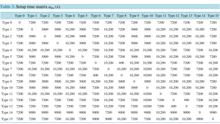
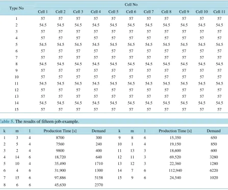
Demands based on product types are given in Table 1, capacities of each cell are given in Table 2, and setup time matrix between product types is represented in Table 3. For instance, if product type 2 is produced right after type 1, 3000 seconds needed to prepare a cell for type 2. The unit processing time matrix is given in Table 4 and the results are transferred to Excel sheet by export command of MPL and the results are given in Table 5.
Table 1. Demands of product types.
Type m
1 2 3 4 5 6 7 8 9 10 11 12 13 14 15
Demand dm 850 400 300 1300 240 2370 6220 650 1020 1710 3280 1280 600 640 5158
Table 2. Capacities of production cells.
Cell No
Cell 1 Cell 2 Cell 3 Cell 4 Cell 5 Cell 6 Cell 7 Cell 8 Cell 9 Cell 10 Cell 11
Capacity hl
(s/month)
[image:4.595.87.539.469.724.2]1,555,200 1,652,400 1,458,000 1,555,200 1,458,000 1,691,280 1,535,760 1,477,440 1,594,080 1,613,520 1,574,640
Table 3. Setup time matrix akm (s).
Type 0 Type 1 Type 2 Type 3 Type 4 Type 5 Type 6 Type 7 Type 8 Type 9 Type 10 Type 11 Type 12 Type 13 Type 14 Type 15
Type 0 0 7200 7200 7200 7200 7200 7200 7200 7200 7200 7200 7200 7200 7200 7200 7200
Type 1 7200 0 3000 3000 10,200 3000 7200 10,200 7200 3000 3000 10,200 10,200 10,200 10,200 7200
Type 2 7200 3000 0 3000 10,200 3000 7200 10,200 7200 3000 3000 10,200 10,200 10,200 10,200 7200
Type 3 7200 3000 3000 0 10,200 3000 7200 10,200 7200 3000 3000 10,200 10,200 10,200 10,200 7200
Type 4 7200 10,200 10,200 10,200 0 10,200 7200 10,200 7200 10,200 10,200 10,200 7200 7200 7200 10,200
Type 5 7200 3000 3000 3000 10,200 0 7200 10,200 7200 3000 3000 10,200 10,200 10,200 10,200 7200
Type 6 7200 7200 7200 7200 7200 7200 0 10,200 600 10,200 10,200 10,200 7200 7200 7200 10,200
Type 7 7200 10,200 10,200 10,200 10,200 10,200 7200 0 10,200 10,200 10200 10,200 7200 7200 7200 10,200
Type 8 7200 7200 7200 7200 7200 7200 600 10,200 0 10,200 10200 10,200 7200 7200 7200 10,200
Type 9 7200 3000 3000 3000 10,200 3000 10,200 10,200 3000 0 3000 10,200 10,200 10,200 10,200 7200
Type 10 7200 3000 3000 3000 10,200 3000 7200 10,200 3000 3000 0 10,200 10,200 10,200 10,200 7200
Type 11 7200 10,200 10,200 10,200 10,200 10,200 7200 10,200 10,200 10,200 10200 0 7200 7200 7200 10,200
Type 12 7200 7200 7200 7200 7200 7200 7200 10,200 7200 7200 10200 7200 0 900 7200 10,200
Type 13 7200 7200 7200 7200 7200 7200 7200 10,200 7200 7200 10200 7200 600 0 7200 10,200
Type 14 7200 9000 9000 9000 9000 9000 9000 7200 9000 9000 9000 10,200 9000 9000 0 9000
Table 4. Unit Processing time matrix tml (s).
Type No Cell No
Cell 1 Cell 2 Cell 3 Cell 4 Cell 5 Cell 6 Cell 7 Cell 8 Cell 9 Cell 10 Cell 11
1 57 57 57 57 57 57 57 57 57 57 57
2 54.5 54.5 54.5 54.5 54.5 54.5 54.5 54.5 54.5 54.5 54.5
3 57 57 57 57 57 57 57 57 57 57 57
4 57 57 57 57 57 57 57 57 57 57 57
5 54.5 54.5 54.5 54.5 54.5 54.5 54.5 54.5 54.5 54.5 54.5
6 57 57 57 57 57 57 57 57 57 57 57
7 57 57 57 57 57 57 57 57 57 57 57
8 54.5 54.5 54.5 54.5 54.5 54.5 54.5 54.5 54.5 54.5 54.5
9 57 57 57 57 57 57 57 57 57 57 57
10 57 57 57 57 57 57 57 57 57 57 57
11 54.5 54.5 54.5 54.5 54.5 54.5 54.5 54.5 54.5 54.5 54.5
12 57 57 57 57 57 57 57 57 57 57 57
13 57 57 57 57 57 57 57 57 57 57 57
14 54.5 54.5 54.5 54.5 54.5 54.5 54.5 54.5 54.5 54.5 54.5
15 57 57 57 57 57 57 57 57 57 57 57
Table 5. The results of fifteen-job-example.
k m l Production Time [s] Demand k m l Production Time [s] Demand
1 3 4 8700 300 9 8 6 15,350 650
2 5 4 7560 240 10 1 4 19,150 850
3 2 4 9800 400 11 13 3 18,600 600
4 14 6 18,720 640 12 11 3 69,520 3280
5 10 4 35,490 1710 13 12 3 22,360 1280
6 4 6 31,900 1300 14 7 6 112,940 6220
7 15 6 97,886 5158 15 9 6 24,540 1020
8 6 6 45,630 2370
Table 5 indicates the sequence of part types based on cell numbers to provide the minimum total completion time and production times of each type. The results demonstrate that 15 parts can produced in cell 3, 4, and 6 that gives minimum total completion time. According to Table 5, the type sequence in cell 4 {1, 3, 2, 5, 10}, in cell 6 {4, 14, 7, 15, 9, 8, 6}, and in cell 3 {11, 13, 12} give the optimum results. In addition to these results the number of each product type demands can be seen on Table 5.
4. Real-
World Problem
In this section, a real-world example is used to evaluate the performance of the model. To illustrate the effec-tiveness of the mathematical model, we compare the results with current production scheduling results.
This study is completed in an automotive injector factory, in body section. Body section has four main processes which are turning, milling, heat treatment, and special process. Within this project we studied in turn-ing process which is the first step of all body section as a pilot. Turnturn-ing process has 35 different part types and 11 production cells.
4.1. Current Situation
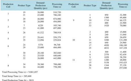
Table 6. Demands, assignments and processing times of current situation.
Production
Cell Product Type
Demand/ Production Quantity (pcs) Processing Time (s) Production
Cell Product Type
Demand/ Production Quantity (pcs)
Processing Time (s)
1 19
21 26,880 43,680 510,720 786,240 9 1 4 10 13 33 850 1300 1710 600 1920 32,300 49,400 64,125 22,500 70,080
2 20
18
46,000 26,000
874,000 494,000
3 7
23
6220 41,000
105,740 697,000
4 26 41,522 788,918
10 2 5 8 11 14 17 25 400 240 650 3280 640 4950 4032 15,000 11,040 26,650 131,200 24,960 188,100 167,328
5 27 35 29,441 12,096 559,379 229,824
6 24
29 5376 25,600 96,768 484,400 7 30 32 22 20,160 25,920 26,000 383,040 440,640 442,000 11 3 6 9 12 15 28 31 300 2370 1020 1280 5158 1344 6048 11,400 92,430 38,250 48,000 193,425 57,120 257,040
8 34
16
39,360 44,600
708,480 758,200
Total Processing Time (s) = 9,861,697
Total Setup Time (s) = 285,600
Total Production Time (h) = 2819
4.2. Proposed Situation
Demands and assignments in current situation are given in Table 6. With the data given in Table 6, we calculate processing times of each type and then we calculate total production time, sum of setup time and processing time, of all types. Table 6 demonstrates that 2819 hours is needed to produce all types regarding to current se-quence table.
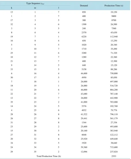
The linear mathematical program with the same demands in current situation is run by MPL and results sum-marized as it is seen in Table 7. Production times in Table 7 consist of processing time and setup time.
According to Table 7, the sequence in cell 1 {19, 7, 18}, in cell 2 {35, 23, 29,}, in cell 4 {8, 6, 16}, in cell 5 {17, 3, 5, 9, 14, 24, 34, 33, 15, 30}, in cell 6 {32, 4, 25, 11, 20}, in cell 7 {13, 1, 2, 10, 12, 22, 21}, and in cell 8 {28, 26, 27, 31} gives the optimum results and the total production time is 2553 hours.
5. Conclusions
In this paper, we have proposed a new method based on linear programming for a parallel machine scheduling problem involving sequence dependent setup times. The criterion is to minimize the total production time. As shown in the real world problem section, total production time reduced from 2819 to 2553 hour. For this prob-lem, average saving based on total production time is 9.4%, and due to the fact that demands are changing every month, the saving will change every month.
Table 7. Results of linear mathematical programming.
Type Sequence ykml
Demand Production Time (s)
k m l
13 1 7 850 19,150
1 2 7 400 9800
17 3 5 300 8700
32 4 6 1300 26,500
3 5 5 240 7560
8 6 4 2370 45,630
19 7 1 6220 112,940
16 8 4 650 13,250
5 9 5 1020 20,340
2 10 7 1710 35,490
25 11 6 3280 71,320
10 12 7 1280 22,360
21 13 7 600 12,300
9 14 5 640 15,120
33 15 5 5158 88,286
6 16 4 44,600 758,800
30 17 5 4950 85,050
7 18 1 26,000 497,000
18 19 1 26,880 516,720
11 20 6 46,000 884,200
22 21 7 43,680 787,140
12 22 7 26,000 442,900
35 23 2 41,000 703,000
14 24 5 5376 102,768
4 25 6 4032 79,776
28 26 8 41,522 796,118
26 27 8 29,441 561,179
31 28 8 1344 27,336
23 29 2 25,600 493,600
15 30 5 20,160 383,940
27 31 8 6048 122,112
20 32 6 25,920 449,640
34 33 5 1920 38,640
24 34 5 39,360 715,680
29 35 2 12,096 237,024
Total Production Time (h) 2553
Another prominent gain is the usage of 8 production cells instead of 11 observed in the current situation. This is achieved by our linear programming approach with optimal product type assignments into production cells.
Figure 1. Comparison of production times [h] (Current vs. Proposed).
Figure 2. Comparison of setup times [h] (Current vs. Proposed).
Acknowledgements
The authors thank BOSCH Bursa Factory for providing data for the problem.
References
[1] Stoop, P. P. M. and Wiers, V.C.S. (1996) The Complexity of Scheduling in Practice. International Journal of Opera-tions and Production Management, 16, 37-53. http://dx.doi.org/10.1108/01443579610130682
[image:8.595.118.508.285.585.2][3] Yang, W.H. and Liao, C.J. (1999) Survey of Scheduling Research Involving Setup Times. International Journal of Systems Science, 30, 143-155. http://dx.doi.org/10.1080/002077299292498
[4] Cheng, T.C.E., Gupta, J.N.D. and Wang, G. (2000) A Review of Flowshop Scheduling Research with Setup Times.
Production and Operations Management, 9, 262-282. http://dx.doi.org/10.1111/j.1937-5956.2000.tb00137.x
[5] Potts, C.N. and Kovalyov, M.Y. (2000) Scheduling with Batching: A Review. European Journal of Operational Re-search, 120, 228-349. http://dx.doi.org/10.1016/S0377-2217(99)00153-8
[6] Bigras, L.P., Gamache, M. and Savard, G. (2008) The Time-Dependent Travelling Salesman Problem and Single Ma-chine Scheduling Problems with Sequence Dependent Setup Times. Discrete Optimization, 5, 685-699.
http://dx.doi.org/10.1016/j.disopt.2008.04.001
[7] Ng, C.T., Cheng, T.C.E. and Kovalyov, M.Y. (2003) Batch Scheduling with Controllable Setup and Processing Times to Minimize Total Completion Time. Journal of the Operational Research Society, 54, 499-506.
http://dx.doi.org/10.1057/palgrave.jors.2601537
[8] Gagne, C., Price, W.L. and Gravel, M. (2002) Comparing an ACO Algorithm with Other Heuristics for the Single Machine Scheduling Problem with Sequence-Dependent Setup Times. Journal of the Operational Research Society, 53, 895-906. http://dx.doi.org/10.1057/palgrave.jors.2601390
[9] Haung, S., Cai, L. and Zhang, X. (2009) Parallel Dedicated Machine Scheduling Problem with Sequence-Dependent Setups and a Single Server. Computers and Industrial Engineering, 58, 165-174.
http://dx.doi.org/10.1016/j.cie.2009.10.003
[10] Tahar, D.N., Yalaoui, F., Chu, C. and Amodeo, L. (2005) A Linear Programming Approach for Identical Parallel Ma-chine Scheduling with Job Splitting and Sequence-Dependent Setup Times. International Journal of Production Eco-nomics, 99, 63-73. http://dx.doi.org/10.1016/j.ijpe.2004.12.007
![Figure 1. Comparison of production times [h] (Current vs. Proposed).](https://thumb-us.123doks.com/thumbv2/123dok_us/8043032.771928/8.595.118.508.285.585/figure-comparison-production-times-h-current-vs-proposed.webp)
