A Simple Generalisation of Kirk’s Approximation for Multi Asset Spread Options by the Lie Trotter Operator Splitting Method

http://dx.doi.org/10.4236/jmf.2014.43016

A Simple Generalisation of Kirk’s

Approximation for Multi-Asset Spread

Options by the Lie-Trotter Operator

Splitting Method

Chi-Fai Lo

Institute of Theoretical Physics and Department of Physics, The Chinese University of Hong Kong, Hong Kong, China

Email: [email protected]

Received 2 March 2014; revised 3 April 2014; accepted 21 April 2014

Copyright © 2014 by author and Scientific Research Publishing Inc.

This work is licensed under the Creative Commons Attribution International License (CC BY). http://creativecommons.org/licenses/by/4.0/

Abstract

In this paper, by means of the Lie-Trotter operator splitting method, we have presented a new unified approach not only to rigorously derive Kirk’s approximation but also to obtain a generali- sation for multi-asset spread options in a straightforward manner. The derived price formula for the multi-asset spread option bears a great resemblance to Kirk’s approximation in the two-asset case. More importantly, our approach is able to provide a new perspective on Kirk’s approxima- tion and the generalization; that is, they are simply equivalent to the Lie-Trotter operator splitting approximation to the Black-Scholes equation.

Keywords

Lognormal Random Variables, Black-Scholes Equation, Spread Options, Kirk’s Approximation, Lie-Trotter Operator Splitting Method

1. Introduction

lognormal random variables. The simplest approach is to evaluate the expectation of the final payoff over the joint probability distribution of the two correlated lognormal underlyings by means of numerical integration. However, practitioners often prefer to use analytical approximations rather than numerical methods because of their computational ease. Among various analytical approximations,e.g. Carmona and Durrleman [1], Deng et al. [2], Bjerksund and Stensland [3], Venkatramana and Alexander [4], Kirk’s approximation seems to be the most widely used and is the current market standard, especially in the energy markets [5]. It is well known that Kirk’s approximation extends from Margrabe’s exchange option formula with no rigorous derivation [6]. Recently, Lo [7] applied the idea of WKB method to provide a derivation of Kirk’s approximation and discuss its validity. Nevertheless, it is not straightforward to provide a generalisation of Kirk’s approximation for the case of multi-asset spread option via this approach.

Accordingly, it is the aim of this paper to present a simple unified approach, namely the Lie-Trotter operator splitting method [8], not only to rigorously derive Kirk’s approximation but also to obtain a generalisation for the case of multi-asset spread option in a straightforward manner. The derived price formula for the multi-asset spread option bears a great resemblance to Kirk’s approximation in the two-asset case. More importantly, the proposed approach is able to provide a new perspective on Kirk’s approximation and the generalisation; that is, they are simply equivalent to the Lie-Trotter operator splitting approximation to the Black-Scholes equation. Illustrative numerical examples for the three-asset spread options are also shown to demonstrate both the accuracy and efficiency of the extended Kirk approximation. Furthermore, it should be emphasized that our approach is completely different from the extended Kirk approximation proposed by Li et al. [9]. Li et al. suggested to approximate the sum of N−1 lognormal assets as a single lognormal variable and then apply Kirk’s approximation directly to this single lognormal variable and the remaining asset to price the N-asset spread option.

2. Two-Asset Spread Options

The price of a European call spread option obeys the two-dimensional Black-Scholes equation

(

)

2 2 2

2 2 2 2

1 1 2 1 2 1 2 2 2 2 1 2

1 2

1 2

1 1

, , 0

2σ F F ρσ σ F F F F 2σ F F r τ P F F τ

 ∂ ∂ ∂ ∂ 

+ + − − =

 

∂ ∂ ∂

∂ ∂

  (1)

with the final payoff condition

(

1, 2, 0

)

max

(

1 2 , 0 .

)

P F F = F −F −K (2) Here F₁ and F₂ are the future prices of the two lognormal underlying assets, σ₁ and σ₂ are the vola- tilities, ρ is the correlation between the two assets, K is the strike price, r is the risk-free interest rate, and

τ

denotes the time-to-maturity. It is well known that no analytical solution is available in closed form and one needs to resort to numerical methods. In the following, we propose a simple derivation of the well-known price formula of Kirk’s approximation by means of the Lie-Trotter operator splitting method [8].

Proposition 1:

The price of the two-asset spread option can be approximated by

(

1, 2,

)

e

{

1

( ) (

1 2

) ( )

2

}

r

P F F

τ

≈ −τ F N

ξ

− F +K N

ξ

(3) where

2 1

1

2

1 1

ln

2

F F K

ξ σ τ

σ τ₋ −

   

 

=   ₊ + 

   

  

 (4)

2 1

ξ

= −

ξ σ τ

− (5)

2 2

1 2 1 2 2

σ₋ = σ − ρσ σ +σ (6)

2

2 2

2 .

F F K

σ =σ _ _ +

 

Proof:

In terms of the two new variables

1

1 2 2

2

and ,

F

R R F K

F K

= = +

+ (8)

Equation (1) can be rewritten as follows:

(

)

0 1 1 2

ˆ ˆ _{, , 0,}

L L r P R R

τ

τ

∂

 _{+ − −}  ₌

 _∂ 

  (9)

where

2 2 2

0 1 2

1 1

ˆ 2

L R

R

σ₋ ∂

=

∂

 (10)

(

)

(

)

2 2

2 2

1 2 2 2 1 2 2 1 2 1 2 2 1

1 2 1

2 1

ˆ _.

2

L R R R R

R R R

R

σ ∂ ρσ σ σ ∂ ρσ σ σ ∂

= + − − −

∂ ∂ ∂

∂

     (11)

The final payoff condition now becomes

(

1, 2, 0

)

2max

(

1 1, 0 .

)

P R R =R R − (12) Accordingly, the formal solution of Equation (9) is given by

(

1, 2,

)

e exp

{

(

ˆ0 ˆ1

)

}

2max

(

1 1, 0 .

)

r

P R R

τ

= −τ

τ

L +L R R − (13)

Since the exponential operator exp

{

τ

(

Lˆ₀+Lˆ₁

)

}

is difficult to evaluate, the Lie-Trotter operator splitting method [8] can be applied to approximate the operator by (see the Appendix)

{ } { }

0 1

ˆLT _exp ˆ _exp ˆ

O = τL τL (14)

and obtain an approximation to the formal solution P F F

(

₁, ₂,

τ

)

, namely

(

1, 2,

)

ˆ 2max

(

1 1, 0

)

2exp

{ }

ˆ0 max

(

1 1, 0

)

2

(

1,

)

,

LT LT

P R R τ =O R R − =R τL R − ≡R C R τ (15) for

(

)

{ }

(

)

(

)

1 2 1 1 2 1 2 1

ˆ _{max 1, 0 0 exp} ˆ _{max 1, 0 max 1, 0 .}

L R R − = ⇒ τL R R − =R R − (16)

It is not difficult to recognise that C R

(

₁,

τ

)

satisfies the partial differential equation

(

)

2 2 2

1 2 1

1 1

, 0

2σ−R R r τ C R τ

 ∂ ∂ 

− − =

 _∂ 

∂

   (17)

with the initial condition: C R

(

₁, 0

)

=max

(

R₁−1, 0

)

, and that the admissible solution is given by

(

1,

)

e

{

1

( )

1

( )

2

}

,

r

C R

τ

= −τ R N

ξ

−N

ξ

(18) where N

( )

⋅ is the cumulative normal distribution function and

2

1 1

1 1

ln 2 R

ξ σ τ

σ τ −

−

 

=  + 

  

 (19)

2 1 .

ξ

= −

ξ σ τ

− (20)

As a result, we obtain

(

1, 2,

)

e 2

{

1

( )

1

( )

2

}

LT r

P R R

τ

= −τR R N

ξ

−N

ξ

(21) which is exactly the approximate price formula given in Equation (3). (Q.E.D.)

to be identical to the price formula of Kirk’s approximation

(

1, 2,

)

1

( )

1

(

2 e

)

( )

2

r Kirk

P S S

τ

=S N d − S +K −τ N d (22) where

(

)

1 2

1

ln ln e ₁

2

r

S S K

d τ σ τ σ τ − − − − +

= + (23)

2 1

d =d −

σ τ

− (24)

2 2

1 2 1 2 2

σ− = σ − ρσ σ +σ (25)

2 2 2 2 . e r S S K τ

σ =σ _{ −} _ +

  (26)

It should be noted that for the Lie-Trotter operator splitting approximation to be valid,

σ τ

₋2 needs to be sufficiently small, namely

σ τ

−2 1. In accordance with Equation (25), this implies that Kirk’s approximation is

more favourable for positive correlation ρ between the two assets. Furthermore, for K=0, the operators Lˆ₀ and

1 ˆ

L commute so that the Lie-Trotter splitting approximation becomes exact and Margrabe’s formula is recovered.

3. Multi-Asset Spread Options

To price a European N-asset call spread option, we need to solve the N-dimensional Black-Scholes equation

(

)

2

1 2

, 1 1

, , , , 0

2

N

ij i j i j N

i j i j

F F r P F F F

F F

ρ σ σ τ

τ =  _{∂ ∂}   _{− −}  ₌  _{∂ ∂ ∂}   



∑

  (27)

subject to the final payoff condition

(

)

1

1 2

1

, , , , 0 max , 0 ,

N

N N j

j

P F F F F F K

−

=

 

= _ − − _



∑



 (28)

where F_i is the future price of the lognormal underlying asset i with the volatility σ_i, ρ_ij is the correlation between the assets i and j, K is the strike price, r is the risk-free interest rate, and

τ

is the time- to-maturity. Unfortunately, this is a very formidable task. In the following, we apply the Lie-Trotter operator splitting method to derive a closed-form approximate price formula for the multi-asset spread option, which bears a great resemblance to the price formula of Kirk’s approximation in the two-asset case.

Proposition 2:

The price of the N-asset spread option can be approximated by

(

)

( )

1

( )

1 2 1 2

1

, , , , e

N r

N N j

j

P F F F τ τ F N θ F K N θ

− − =       ≈  − +       

∑



 (29)

where 2 1 1 1 1 1 ln 2 N N j j F F K

θ σ τ

σ τ − −

− ₌      _{ }  = _ + _  ₊   _{ }  

∑

 (30) 2 1

θ

= −

θ σ τ

− (31)

2 2

2

N N

σ₋ = σ − ρσ σ ₊+σ₊ (32)

1 1 1 1 N j j N j j F F K σ σ − = + + − =     =  ₊   

∑

∑

1 , 1

1 1

N

jk j k j k j k N j j F F F

ρ σ σ σ − = + − = =

∑

∑

 (34)

1 1 1 1 1 . N

jN j j j N j j F F ρ σ ρ σ − = − + ₌     =    

∑

∑



 (35)

Proof:

Introducing the new variables: f_i ≡F_i−F+ for i=1, 2,,N−2 and

1 1

N j j

F+ ≡

∑

=−F , Equation (27) can be

cast in the form

(

1 2

)

ˆ ˆ ˆ ˆ _{, , , , 0,}

N N R N

L L L L r P F F F

τ

τ

+ + ∂

 _{+ + + − −}  ₌

 _∂ 

   (36)

where 2 2 2 2 1 ˆ 2

N N N

N

L F

F

σ ∂

=

∂ (37)

2 2 2 2 1 ˆ 2 L F F σ + + + + ∂ = ∂

 (38)

2 ˆ

N N N

N

L F F

F F ρσ σ + + + + ∂ = ∂ ∂

  (39)

2

2 1 1

1 1 1

2

2 2 1 1 1

1 1 1 1 1

1 ˆ 2 1 2 . 2

N N N

R kn k k mn m m n n

k n m k

N N N N N

kn k k mn m m n n pq p q p q

k n m p q n k

L F F F

F f

F F F F F

f f

ρ σ ρ σ σ

ρ σ ρ σ σ ρ σ σ

− − − = = = + − − − − − = = = = = ∂   = _ − _ ∂ ∂      ∂ +  −  + _{∂ ∂}    

∑ ∑

∑

∑ ∑

∑

∑∑

(40)

The formal solution of Equation (36) is given by

(

1, 2, , ,

)

e exp

{

(

ˆ ˆ ˆ ˆ

)

}

max

(

, 0 .

)

r

N N N R N

P F F  F

τ

= −τ

τ

L +L₊+L ₊+L × F −F₊−K (41)

Then we apply the Lie-Trotter operator splitting method [10] to obtain an approximation to the formal solution

(

1, 2, , N,

)

P F F  F

τ

, namely (see the Appendix)

(

)

(

)

{

}

{ }

(

)

(

)

{

}

(

)

1, 2, , ,

ˆ ˆ ˆ ˆ

e exp exp max , 0

ˆ ˆ ˆ

e exp max , 0 ,

LT

N

r

N N R N

r

N N N

P F F F

L L L L F F K

L L L F F K

τ τ τ τ τ τ − + + + − + + + = + + − − = + + − −  (42)

where the relation

(

)

{ }

(

)

(

)

ˆ _{max , 0 0 exp} ˆ _{max , 0 max , 0 .}

R N R N N

L F −F+−K = ⇒ τL F −F+−K = F −F+−K (43)

is utilized.

Next, in terms of the two new variables

1 and 2 ,

N F

R R F K

F+ K +

= = +

+ (44)

(

1, 2, , ,

)

e exp

{

(

ˆ ˆ

)

}

2max

(

1 1, 0 ,

)

LT r

N A B

P F F  F

τ

= −τ

τ

L +L R R − (45)

where 2 2 2 1 2 1 1 ˆ 2 A L R R

σ₋ ∂

=

∂ (46)

(

)

(

)

2 2

2 2

2 2 1 2 1

1 2 1

2 1

ˆ 2

B N N

L R R R R

R R R

R

σ₊ ∂ ρσ σ σ_{+ +} ∂ ρσ σ σ_{+ +} ∂

= + − − −

∂ ∂ ∂

∂   (47)

2 2

2

N N

σ₋= σ − ρσ σ ₊+σ₊ (48)

.

F F K

σ σ +

+ + +   = _{ } +  

 (49)

It is clear that the exponential operator exp

{

τ

(

Lˆ_A+Lˆ_B

)

}

is difficult to evaluate, so we need to apply the

Lie-Trotter operator splitting method [10] again to approximate the operator by exp

{ } { }

τLˆA exp τLˆB . As a result, we obtain

(

)

{ } { }

(

)

{ }

(

)

1 2 2 1

2 1

ˆ ˆ

, , , , e exp exp max 1, 0

ˆ

e exp max 1, 0

LT r

N A B

r

A

P F F F L L R R

R L R

τ

τ

τ τ τ

τ − − ≈ − ≈ −  (50) for

(

)

{ }

(

)

(

)

2 1 2 1 2 1

ˆ _{max 1, 0 0 exp} ˆ _{max 1, 0 max 1, 0 .}

B B

L R R − = ⇒ τL R R − =R R − (51)

Since σ₋ is independent of R₁, the standard workhorse of the Black-Scholes model can be used to evaluate

{ }

ˆ

(

1

)

exp τLA max R −1, 0 such that

(

1, 2, , ,

)

e 2

{

1

( )

1

( )

2

}

LT r

N

P F F  F

τ

≈ −τR R N

θ

−N

θ

(52) where 2 1 1 1 ln 2 N F F K

θ σ τ

σ τ− + −

   

 

= _{  }+ _

+

   

  (53)

2 1 .

θ

= −

θ σ τ

− (54)

It is obvious that this approximate solution is identical to the approximate price formula given in Equation (29). (Q.E.D.)

In terms of the spot asset prices, namely Si≡Fiexp

(

−r

τ

)

, the price formula given in Equation (29) becomes

(

)

( )

1

( )

1 2 1 2

1

, , , , e

N

r

Kirk N N j

j

P S S S τ S N d S K τ N d

− − =   = −_ + _ 

∑



 (55)

where

(

1

)

1 1

ln ln e ₁

ˆ 2 ˆ

N r

N j j

S S K

d τ σ τ σ τ − − = − − − +

=

∑

+ (56)

2 1 ˆ

d =d −

σ τ

− (57)

2 2

ˆ N 2 N ˆ ˆ

σ₋= σ − ρσ σ₊+σ₊ (58)

1 , 1 1 1 ˆ e N

jk j k j k j k

N r

j j

S S

S K τ

ρ σ σ σ − = + − − = = +

∑

1 1

1 1 1

. ˆ

N

jN j j j

N j j

S

S

ρ σ ρ

σ

− =

−

+ ₌

 

 

=

 

 

∑

∑

(60)

Obviously, this approximate price formula resembles the price formula of Kirk’s approximation in the two-asset case very closely. In fact, by setting N=2 we can recover Kirk’s approximation readily. Moreover, for the Lie-Trotter splitting approximation to be valid, we need to require

σ τ

ˆ₋2 to be sufficiently small, namely

2 1

σ τ

−  . In accordance with Equation (58), this implies that the extended Kirk approximation is more

favourable for those cases with positive effective correlation

ρ

.

4. Illustrative Numerical Examples for the Three-Asset Spread Options

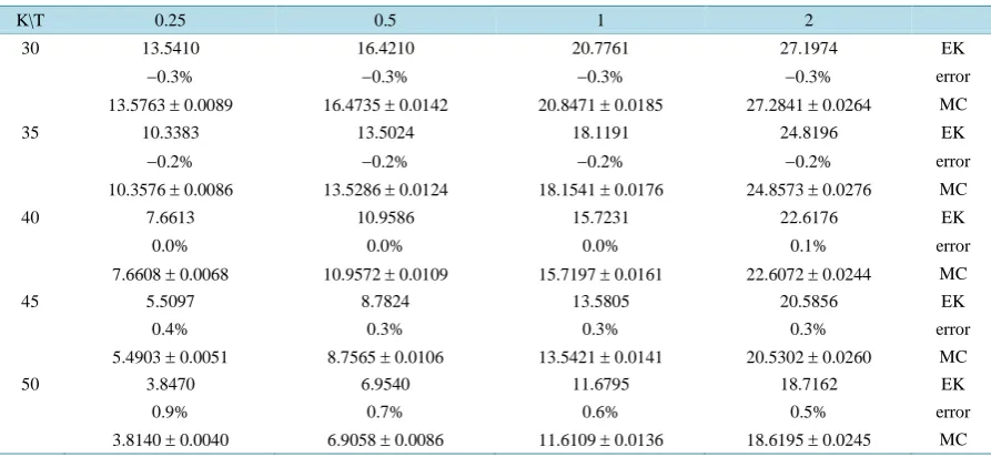
In this section, illustrative numerical examples are presented to demonstrate the accuracy of the extended Kirk approximation for the three-asset spread options. Although most spread options involve two assets only, yet there is a growing demand for three-asset spread options which can be found in the models for power plants or their financial equivalents—tolling contracts. We examine a simple three-asset spread option with the final payoff max

(

S3− −S1 S2−K, 0

)

. Table 1 tabulates the approximate option prices estimated by the extended

Kirk approximation for different values of the strike price K and time-to-maturity T. Other input model parameters are set as follows: r=0.05, σ₁=σ₂=σ₃=0.3, ρ =₁₂ 0.4, ρ =₂₃ 0.2, ρ =₁₃ 0.8, S₁=50,

2 60

S = and S₃ =150. Monte Carlo estimates and the corresponding standard deviations are also presented for comparison. It is observed that the computed errors of the approximate option prices are capped at 1% (in magnitude). In fact, most of them are less than 0.5%. Then, in Table 2 the effect of increasing the three vol- atilities (from 0.3 to 0.6) upon the approximate estimation of the option prices is investigated. Obviously only a slight increase occurs in the computed errors, and these errors are still less than 1% (in magnitude). Finally, we study a case in which all the three volatilities are different, namely σ =₁ 0.5, σ =₂ 0.4 and

3 0.3

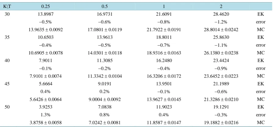
σ = , while the other parameters remain the same. According to Table 3, the computed errors generally increase a little bit in this case but they do not exceed 1.3% (in magnitude). As a result, it can be concluded that the extended Kirk approximation for the three-asset spread option is found to be very accurate and efficient.

5. Conclusion

[image:7.595.90.537.512.718.2]

In this paper, we have proved that Kirk’s approximation for two-asset spread options can be rigorously derived

Table 1. Prices of a European three-asset call spread option. Other input parameters are: r = 0.05, σ1 = σ2 = σ3 = 0.3, ρ12 =

0.4, ρ23 = 0.2, ρ13 = 0.8, S1 = 50, S2 = 60 and S3 = 150. Here “EK” refers to the extended Kirk approximation while “MC”

denotes the Monte Carlo estimates with 900,000,000 replications. The relative errors of the “EK” option prices with respect to the “MC” estimates are also presented.

K\T 0.25 0.5 1 2

30 13.5410 16.4210 20.7761 27.1974 EK

−0.3% −0.3% −0.3% −0.3% error

13.5763 ± 0.0089 16.4735 ± 0.0142 20.8471 ± 0.0185 27.2841 ± 0.0264 MC

35 10.3383 13.5024 18.1191 24.8196 EK

−0.2% −0.2% −0.2% −0.2% error

10.3576 ± 0.0086 13.5286 ± 0.0124 18.1541 ± 0.0176 24.8573 ± 0.0276 MC

40 7.6613 10.9586 15.7231 22.6176 EK

0.0% 0.0% 0.0% 0.1% error

7.6608 ± 0.0068 10.9572 ± 0.0109 15.7197 ± 0.0161 22.6072 ± 0.0244 MC

45 5.5097 8.7824 13.5805 20.5856 EK

0.4% 0.3% 0.3% 0.3% error

5.4903 ± 0.0051 8.7565 ± 0.0106 13.5421 ± 0.0141 20.5302 ± 0.0260 MC

50 3.8470 6.9540 11.6795 18.7162 EK

0.9% 0.7% 0.6% 0.5% error

[image:8.595.92.540.131.346.2]

Table 2. Prices of a European three-asset call spread option. Other input parameters are: r = 0.05, σ1 = σ2 = σ3 = 0.6, ρ12 =

0.4, ρ23 = 0.2, ρ13 = 0.8, S1 = 50, S2 = 60 and S3 = 150. Here “EK” refers to the extended Kirk approximation while “MC”

denotes the Monte Carlo estimates with 900,000,000 replications. The relative errors of the “EK” option prices with respect to the “MC” estimates are also presented.

K\T 0.25 0.5 1 2

30 20.1436 26.0640 34.5186 46.3820 EK

−0.3% −0.3% −0.1% 0.3% error

20.2066 ± 0.0168 26.1269 ± 0.0278 34.5402 ± 0.0425 46.2242 ± 0.0716 MC

35 17.4529 23.5976 32.2944 44.4495 EK

−0.1% 0.0% 0.1% 0.5% error

17.4778 ± 0.0172 23.6076 ± 0.0268 32.2508 ± 0.0390 44.2275 ± 0.0787 MC

40 15.0417 21.3320 30.2150 42.6221 EK

0.1% 0.2% 0.4% 0.7% error

15.0290 ± 0.0171 21.2938 ± 0.0266 30.1079 ± 0.0362 42.3425 ± 0.0656 MC

45 12.9002 19.2587 28.2733 40.8938 EK

0.4% 0.4% 0.6% 0.9% error

12.8527 ± 0.0182 19.1753 ± 0.0234 28.1113 ± 0.0381 40.5466 ± 0.0628 MC

50 11.0139 17.3676 26.4620 39.2590 EK

0.7% 0.7% 0.8% 1.0% error

10.9347 ± 0.0151 17.2410 ± 0.0236 26.2513 ± 0.0345 38.8658 ±0.0637 MC

Table 3. Prices of a European three-asset call spread option. Other input parameters are: r = 0.05, σ1 = 0.5, σ2 = 0.4, σ3 = 0.3,

ρ12 = 0.4, ρ23 = 0.2, ρ13 = 0.8, S1 = 50, S2 = 60 and S3 = 150. Here “EK” refers to the extended Kirk approximation while

“MC” denotes the Monte Carlo estimates with 900,000,000 replications. The relative errors of the “EK” option prices with respect to the “MC” estimates are also presented.

K\T 0.25 0.5 1 2

30 13.8987 16.9731 21.6091 28.4620 EK

−0.5% −0.6% −0.8% −1.2% error

13.9635 ± 0.0092 17.0801 ± 0.0119 21.7922 ± 0.0191 28.8014 ± 0.0242 MC

35 10.6503 13.9613 18.8011 25.8630 EK

−0.4% −0.5% −0.7% −1.1% error

10.6905 ± 0.0078 14.0301 ± 0.0118 18.9316 ± 0.0163 26.1380 ± 0.0238 MC

40 7.9011 11.3085 16.2480 23.4424 EK

−0.1% −0.2% −0.4% −0.9% error

7.9101 ± 0.0074 11.3342 ± 0.0104 16.3206 ± 0.0172 23.6452 ± 0.0223 MC

45 5.6664 9.0191 13.9501 21.1989 EK

0.4% 0.2% −0.1% −0.6% error

5.6426 ± 0.0064 9.0004 ± 0.0092 13.9627 ± 0.0145 21.3286 ± 0.0210 MC

50 3.9253 7.0838 11.9023 19.1291 EK

1.3% 0.8% 0.4% −0.3% error

3.8758 ± 0.0058 7.0242 ± 0.0081 11.8587 ± 0.0147 19.1882 ± 0.0216 MC

[image:8.595.92.540.400.609.2]

examples, the generalization is found to be very accurate and efficient in pricing the multi-asset spread options. All in all, our approach is able to provide a new perspective on Kirk’s approximation and the generalisation; that is, they are simply equivalent to the Lie-Trotter operator splitting approximation to the Black-Scholes equation.

References

[1] Carmona, R. and Durrleman, V. (2003) Pricing and Hedging Spread Options. SIAM Review, 45, 627-685.

http://dx.doi.org/10.1137/S0036144503424798

[2] Deng, S.J., Li, M. and Zhou, J. (2008) Closed-Form Approximation for Spread Option Prices and Greeks. Journal of Derivatives, 15, 58-80. http://dx.doi.org/10.3905/jod.2008.702506

[3] Bjerksund, P. and Stensland, G. (2011) Closed Form Spread Option Valuation. Quantitative Finance, iFirst, 1-10. [4] Venkatramana, A. and Alexander, C. (2011) Closed form Approximation for Spread Options. Applied Mathematical

Finance, 18, 447-472. http://dx.doi.org/10.1080/1350486X.2011.567120

[5] Kirk, E. (1995) Correlation in the Energy Markets. Managing Energy Price Risk. Risk Publications and Enron, London, 71-78.

[6] Margrabe, W. (1978) The Value of an Option to Exchange One Asset for Another. Journal of Finance, 33, 177-186.

http://dx.doi.org/10.1111/j.1540-6261.1978.tb03397.x

[7] Lo, C.F. (2013) A Simple Derivation of Kirk’s Approximation for Spread Options. Applied Mathematics Letters, 26, 904-907. http://dx.doi.org/10.1016/j.aml.2013.04.004

[8] Trotter, H.F. (1958) Approximation of Semi-Groups of Operators. Pacific Journal of Mathematics, 8, 887-919.

http://dx.doi.org/10.2140/pjm.1958.8.887

[9] Li, M., Zhou, J. and Deng, S.J. (2010) Multi-Asset Spread Option Pricing and Hedging. Quantitative Finance, 10, 305-324. http://dx.doi.org/10.1080/14697680802626323

[10] Trotter, H.F. (1959) On the Product of Semi-Groups of Operators. Proceedings of the American Mathematical Society,

10, 545-551. http://dx.doi.org/10.1090/S0002-9939-1959-0108732-6

[11] Suzuki, M. (1985) Decomposition Formulas of Exponential Operators and Lie Exponentials with Some Applications to Quantum Mechanics and Statistical Physics. Journal of Mathematical Physics, 26, 601-612.

http://dx.doi.org/10.1063/1.526596

[12] Drozdov, A.N. and Brey, J.J. (1998) Operator Expansions in Stochastic Dynamics. Physical Review E, 57, 1284-1289.

http://dx.doi.org/10.1103/PhysRevE.57.1284

[13] Hatano, N. and Suzuki, M. (2005) Finding Exponential Product Formulas of Higher Orders. Lecture Notes in Physics,

679, 37-68.

[14] Blanes, S., Casas, F., Chartier, P. and Murua, A. (2013) Optimized Higher-Order Splitting Methods for Some Classes of Parabolic Equations. Mathematics of Computation, 82, 1559-1576.

Appendix: Lie-Trotter Operator Splitting Method

Suppose that one needs to exponentiate an operator Cˆ which can be split into two different parts, namely Aˆ

and Bˆ. For simplicity, let us assume that Cˆ= +Aˆ Bˆ, where the exponential operator exp

( )

Cˆ is difficult to evaluate but exp

( )

Aˆ and exp

( )

Bˆ are either solvable or easy to deal with. Under such circumstances, the

exponential operator exp

( )

εCˆ , with

ε

being a small parameter, can be approximated by the Lie-Trotter operator splitting formula:

( )

_ˆ

( ) ( )

_{ˆ ˆ}

( )

2

exp εC =exp εA exp εB +O ε . (A.1)