Capital liberalization, industrial agglomeration and wage inequality

Munich Personal RePEc Archive

Capital liberalization, industrial

agglomeration and wage inequality

Li, Yao

University of Hawaii at Manoa, University of Electronic Science and

Technology of China

December 2007

Online at

https://mpra.ub.uni-muenchen.de/11355/

Capital Liberalization, Industrial Agglomeration

and Wage Inequality

Abstract: This paper sets up a new economic geography model with diminishing

marginal returns and examines the effect of capital liberalization on industrial

agglomeration and wage inequality. The simulation results indicate that for the country

with strict capital controls, capital liberalization can help reduce wage difference between

countries in both nominal and real terms. It is also shown that when both comparative

advantage and agglomeration are in effect, low trading costs does not necessarily cause

the catastrophic agglomeration in the country with the larger market as most other NEG

models predict.

Key Words: New Economic Geography, Capital Liberalization, Trade Costs

JEL Classification: F12, O24, R12

1. Introduction

In the 1990s, theorists developed a new approach to understanding the spatial

concentration of economic activities: "New Economic Geography" (NEG). NEG

approaches economic geography with a perspective developed from "new trade theory"

instead of regional economics. Most of the NEG models predict that a larger economy

(i.e., one has both a greater labor endowment and a larger local market) tends to be more

attractive to manufactures and to offer higher real wage levels. NEG models successfully

explain the geographical distribution of economic activities among countries within the

European Union as well as counties within the United States [Baldwin et. al. (2003),

Henderson and Thisse (2004)]. However, the stylized facts of China seem to run contrary

The economy of China is larger than most of its trading partners. The country also

has the largest labor endowment in the world. But the labor costs (real wage level) of

China are lower than most of its trading partners. This is consistent with the prediction of

the traditional Hecksher-Olin trade theory. The H-O theory is based on an important

assumption, diminishing marginal returns, which is a law followed by most production

systems. The law of diminishing returns states that in a production system with fixed and

variable inputs, beyond some point, each additional unit of variable input yields less and

less additional output. The existence of diminishing marginal returns affects the

equilibrium factor returns and location of production materials. It will impede the use of

inputs that exceeds the optimal level indicated by the given technology. In other words, it

can impede the agglomeration of factors and economic activities to some extent.

Therefore, it is necessary to include the second factor, capital, into the NEG models when

analyzing the causes of agglomeration and the resulting equilibrium factor returns. Some

theorists have set up NEG models involving both labor and capital (either physical or

human capital) in industrial production, such as Martin and Rogers’s (1995) Footloose

Capital (FC) model, Ottaviano (1996) and Forslid’s (1999) Footloose Entrepreneurs (FE)

model and Baldwin’s (1999) Constructed Capital (CC) Model. However, none of these

studies focus on the interaction between agglomeration and diminishing marginal returns.

In this paper, I set up a NEG model with diminishing marginal returns and examine the

effect of capital liberalization on industrial agglomeration and wage inequality. Amiti

(2005) also embed a NEG model with vertical linkages within a Heckscher-Ohlin

But her study focuses on the effects of reducing trade costs rather than the capital

mobility on the location of manufacturing firms.

On the other hand, most NEG models predict catastrophic agglomeration

[Baldwin (1999)] of manufactures when the trade costs are sufficiently low. This does not

seem to find empirical support at a broad. As a “world factory”, China is attractive to the

labor-intensive industries. However, it is unlikely that China will attract a relocation of

all labor-intensive industries, much less a relocation of all manufacturing industries, into

China. In the labor-involved production, the shift of production can lead to the shift of

both labor and expenditure, which followed by further production shifting. This kind of

circular causality finally causes the catastrophic agglomeration. By introducing capital as

a specific factor for the final manufacturing production, my model divides the

manufacturing sector into labor- and capital- intensive industries and completely rules out

the circular causality from the capital-intensive industry. As a result, my simulation

results show that only if the distribution of labor endowments is highly concentrated and

the trade costs are extremely low, the labor-intensive industries agglomerate into the

labor abundant countries. The catastrophic agglomeration does not occur in the

capital-intensive industries.

The remainder of the paper is organized as follows. In the second section, I

incorporate a capital endowment into Puga (1999) 's Core-Periphery model with Vertical

Linkage (CPVL) and set up an autarky model with three factors and two sectors. In the

third section, the model is expanded to include two countries and international trade.

robustness of the model to the introduction of trade costs for agricultural goods.

Conclusions and remarks are in section four.

2. Model of Autarky Economy

To set up a model with international trade, I start from a model of an autarky

economy. Consider a model similar to Puga (1999)'s model, with two sectors, agriculture

and manufacturing, but three factors, arable land (A), labor (L) and capital (K), instead of

two factors (land and labor).1 _{Labor is assumed to be mobile between the agricultural}

sector and manufacturing sector which is the assumption also used by Puga. I assume

land and capital are specific factors for agriculture and manufacturing respectively.

1. Consumer Side

As in the CPVL model, the representative consumer maximizes utility:

μ μ

M A C

C

U = 1− _{, 0}<μ <_{1 (2.1)}

s.t P_AC_A +P_MC_M =Y (2.2)

where C_Aand C_M denote the consumption of agricultural products and final

manufactures. P_A and P_M are prices of agricultural products and final manufactures and

Y is the income.

The utility function implies that μ share of a representative consumer's income

will be spent on manufactures and 1−μ share of the income will be spent on agricultural

products. Assume everybody in the economy has the same utility function. The share of

manufactures in the total consumption of the economy will beμ.

2. Producer Side

1

Agriculture is perfectly competitive and produces a homogenous output with a

constant return to scale (CRS) technology as in the CPVL model. I use the specific

production function that Puga (1999) uses for the agricultural sector: X_A = A1−θ θL_A. XA, A

and LA denote the agricultural output, the amount of arable land and the labor employed

in the agricultural sector respectively. Since the land endowment is fixed, the

representative land owner will choose the amount of labor to maximize the return to land

(g) according to the prevailing wage level (w) and agricultural commodity price (P_A).

Same as all other NEG models, the price of the agricultural product is set to be the

numeraire: PA = 1. So the maximization problem for a representative land owner is:

Max ( )Ag w =X P_{A A}−wL_A, s.t. X_A ≤A1−θ θL_A. (2.3)

The manufacturing sector displays increasing return to scale (IRS) in a two-stage

production process: As in the CPVL model, the first stage products are differentiated

intermediate manufactures that will be used as inputs in the second stage of production.

The number of varieties of the first stage manufactures is endogenous. The second stage,

however, involves a Cobb-Douglas combination of the intermediate manufactures (C_L)

and capital which is not considered in the CPVL and most related models.

Following Krugman (1991) and all other NEG models, I use Dixit and Stiglitz

(1977)'s framework to model the intermediate manufacturing production, which implies

that each variety can be produced by only one firm. The production of an individual

variety involves a fixed cost and a constant marginal cost: to produce x_i of good i, I need

i

i x

The total cost of producing good i is E_i =wL_i= )w(α +βx_i , so the marginal cost

is i

i i E MC x ∂ =

∂ = wβ. Therefore the IRS of first stage manufactures comes from the scale

of a single firm's production.

Following Krugman (1991), the aggregation of intermediate manufactures is

defined by 1 1 1 ₋ = − ⎟⎟ ⎠ ⎞ ⎜⎜ ⎝ ⎛

=

∑

σ σ σ n i i L c

C (2.4)

where n is the number of varieties of intermediate manufactures and σ > 1 is the elasticity

of substitution among the varieties. 2

The price index of intermediate manufactures can be defined as [Fujita et.al.

(1999)]: PL =

σ σ − = − _⎟ ⎠ ⎞ ⎜ ⎝ ⎛

∑

The production function of final manufactures is defined as:

b b n i i b b L

M C K c K

X − − = − − ⎥ ⎥ ⎥ ⎦ ⎤ ⎢ ⎢ ⎢ ⎣ ⎡ ⎟ ⎟ ⎠ ⎞ ⎜ ⎜ ⎝ ⎛ =

=

∑

1 1 1 σ σ σ σ (2.6)

where 0<b<1.

By now, I have set up a model of an autarky economy with two sectors and three

factors. The inclusion of both labor and capital as variable input for industrial production

enables the model to reflect the effect of diminishing marginal returns for both labor and

capital. At the same time, since the capital input is specific for the final manufacturing

production, we can certainly consider this industry as the capital-intensive industry while

2

the intermediate manufacturing production is labor-intensive. This division strengthens

the difference of the two vertically linked industries and further help in analyzing the

special distribution of labor- and capital-intensive industries separately. In the following

section, I solve the general equilibrium and do some comparative static analysis.

3. General Equilibrium and Comparative Static Analysis

Same as the standard Dixit-Stiglitz (1977) framework, I assume the producer of

each variety acts as though his behavior does not influence that of other varieties’

producers. By solving the production maximization problem, I can get the profit

maximization price for each variety of the intermediate manufacture:

σ 1 ⎟⎟ ⎠ ⎞ ⎜⎜ ⎝ ⎛ = i L i nc C

p (2.7)

and the optimized production for each variety: x_i α σ( 1) β

= − . (2.8)

(It is the same with most NEG models.)

Therefore, the number of varieties:

n = i A L L L− = i w x Ag L β α + − = ασ w Ag L− = ασ θ θ 1 1 − ⎟ ⎠ ⎞ ⎜ ⎝ ⎛ −A w L

. (2.9)

Assume that the market for final manufactures is perfectly competitive. The zero

profit condition is:

b rK b C P rK C P X

P L L

L L M

M = + = = ₋

1 . (2.10)

Market clearing in autarky implies

A

A C

X = , (2.11)

i i

M

M X

C = . (2.13)

Full employment implies:

∑

= + = n i i A L L L 1

. (2.14)

Balance of payment gives us: P_AC_A +P_MC_M = Ag(w)+Lw+Kr. (2.15)

Solving the system (2.11) - (2.15), I get the equilibrium factor returns, commodity

prices and the number of varieties.

The equilibrium wage rate:

θ θ θ μ θ − − ⎥ ⎦ ⎤ ⎢ ⎣ ⎡ + ⎟⎟ ⎠ ⎞ ⎜⎜ ⎝ ⎛ ₋ − ⎟ ⎠ ⎞ ⎜ ⎝ ⎛ = 1 1 1 1 1 1 b L A

w . (2.16)

The equilibrium land price:

θ θ θ θ θ μ θ θ θ ⎟ ⎠ ⎞ ⎜ ⎝ ⎛ ⎥ ⎦ ⎤ ⎢ ⎣ ⎡ + ⎟⎟ ⎠ ⎞ ⎜⎜ ⎝ ⎛ − − − = − = − − A L b w w

g 1 1

1 1 ) 1 ( ) )( 1 ( )

( /( 1) . (2.17)

The equilibrium capital rent:

1 1

(1 ) ( )

(1 )

b b L A

r

K

θ θ θ θ

θ

μ θ μ θ μθ

μ

− −

−

− + −

=

− . (2.18)

The price and price index of intermediate manufactures:

(

)

1 1 1 ) 1 ( 1 1 ) 1 1 1 ( 1 1 1 ) 1 ( − − − + − − − + − − − − ⎟⎟ ⎠ ⎞ ⎜⎜ ⎝ ⎛ − + =

= _σ θ _σ σ θ θ θ σ θ

σ σ β μ θ μ ασ μθ θ

μ A L

b b

p n

P_{L i} (2.19)

The equilibrium price of final manufactures: ₌ 1− − −1 b−1 b

M A L K

P σ

σ θ θ

ξ (2.20)

where

(

)

σ σ

σ θ

θ _{μ θ μθ}

σ α β μ ασ μ μθ ξ − − − − _{+ −} ⎟⎟ ⎠ ⎞ ⎜⎜ ⎝ ⎛ − ⎟⎟ ⎠ ⎞ ⎜⎜ ⎝ ⎛ − = 1 1 1 ) 1 ( ) 1 ( b b b b b

And the number of varieties of intermediate manufactures:

( )

Lb n

b

μ μ θ μθ ασ

=

From the comparative static analysis, I can get some standard results of traditional

trade theories:

i) The price of a factor decreases in the factor's endowment ( ( ) <0

∂ ∂

A w g

, w 0

L ∂ _< ∂ , 0 < ∂ ∂ K r

) and increases in other factors’ endowments ( ( ) >0

∂ ∂

L w g

, w 0

A ∂ _>

∂ , ∂ >0 ∂ A r , 0 > ∂ ∂ L r ).

ii) The price of a product decreases in the supply of its inputs

( <0

∂ ∂

L P_L

, <0

∂ ∂

K P_M

, <0

∂ ∂

L P_M

if θ <b) and increases in the supply of other products’

inputs ( >0

∂ ∂

A P_L

, >0

∂ ∂

A P_M

).3

I can also get some results that are consistent with previous CPVL model:

i) The equilibrium wage and the number of varieties increase in the share of

industry in the economy ( μ

∂ ∂w

>0, n 0 μ

∂ _>

∂ ). But the land rent decreases in the share of

industry in the economy ( ( )<0

∂ ∂ μ w g ).

ii) The number of varieties increases in the labor endowment ( n 0

L ∂

>

∂ ) and

decreases in the firm-level economies of scale (α ).

At the same time, due to the involvement of capital in the model, I also get some

new results:

3

Proposition 1. As the share of intermediate manufactures in the cost of final

manufacturing production increase, the equilibrium wage rate increase ( w 0

b ∂

>

∂ ), while

the equilibrium land and capital rent decreases ( ( ) <0

∂ ∂

b w g

, <0

∂ ∂ b r

).

Holding all else equal, as the cost share of intermediate manufactures increases,

the labor needed in manufacturing production will increase. Therefore, the return to labor

increases, while the return to other factors (arable land and capital) decrease.

From (2.19) and (2.20), I can have the price ratio of final and intermediate

manufactures: 1 1 1 1 1 1 1 1 ₁ ) ( − − − − − − − − − ⎟⎟ ⎠ ⎞ ⎜⎜ ⎝ ⎛ − ⎥ ⎦ ⎤ ⎢ ⎣ ⎡ − + = b b b b b b i

M _{b b L K}

p

P σ _{σ σ}σ _σσ

σ α β σ θ μ θ

σ (2.22)

Therefore ⎩ ⎨ ⎧ < − σ < > − σ > ∂ ∂ 1 ) 1 ( , 0 1 ) 1 ( , 0 b if b if L p P i M

and <0

∂ ∂ K p P i M

. (2.23)

Equation (2.23) indicates that the increase of capital endowment will decrease the

relative prices of final manufacturing products (based on the price of intermediate

manufactures). However, the relationship between labor endowment and the relative

prices of final manufacturing products is uncertain and depends on the elasticity of

substitution among varieties (σ) and the cost share of capital in industrial production

(1−b). If σ(1−b)>1, the increase of labor endowment will increase the relative prices of

final manufacturing products. In other words, if the elasticity of substitution or the costs

share of capital in industrial production is sufficiently large, the increase of labor

Proposition 2. Keeping other conditions unchanged, if σ(1−b)>1, a country with more

labor will have higher relative prices of final manufactures (based on the price of

intermediate manufactures) than if the country would have a less labor endowment.

In this section, I set up a model of an autarky economy based on the framework of

Puga (1999)'s CPVL model. I introduce a second factor, capital, as variable input for

manufactures which makes my model different from the NEG models with only one

industrial input. Therefore, besides the results similar with that of traditional trade

theories and previous CPVL model, my model also presents the effects of capital and

diminishing marginal returns on the economy.

3. The Two-Country Model

3.1.The Two-Country Model with Immobile Factors

Now consider a two-country (x, y) model. Assume country y has more labor than

country x. Other endowments and technology are the same for these two countries. Also

assume that all products can be traded across countries but all factors cannot. Labor is

still mobile across agriculture and manufacturing. Land and capital are specific factors

for agriculture and manufacturing respectively.

From the previous section, I know that in autarky, country y will have a lower

wage rate and manufacture prices,4 _{but higher prices of capital and land. Use subscript x,}

y to distinguish each variable for different countries. From (2.19), (2.22) and (2.23), I

know that in autarky, if σ(1−b)>1, I have

Ax Ay

Mx My

x y

P P

P P

p p

<

< . Thus the order of

comparative advantage of country y's products will be intermediate manufactures > final

4

manufactures > agricultural products. Therefore, country y will be a net exporter of

intermediate manufactures and a net importer of agricultural products if the two countries

trade with each other. The trade direction of final manufactures is uncertain. On the other

hand, if σ(1−b)<1, I have

Ax Ay

x y

Mx My

P P

p p

P P

<

< . Then country y will be a net exporter of

final manufactures and still a net importer of agricultural products in trade. The trade

direction of intermediate manufactures is uncertain. So, besides the endowment, both the

elasticity of substitution among varieties and the utilization of capital in industrial

production can affect a country's trade pattern.

LetL_k,w_k, K_k, r_kdenote the endowments and factor prices in country k (k = x, y).

Following the standard CP model, agricultural products can be traded costlessly, so I use

their price as the numeraire again: PA = 1. All manufactures can trade at "iceberg" trade

costs. Only τ (0<τ <1) share of shipped goods can be delivered from one country to the

other country. The production of the agricultural and manufacturing sectors and the

utility function are the same with the autarky economy.

The number of varieties of the first stage manufactures produced in country k is

k

n . The assumption of monopolistic competition implies that one variety can only be

produced in one region and by one firm [Dixit and Stiglitz (1977)], so the total number of

intermediate manufacturing varieties is n=n_x+n_y.

Similarly with the autarky economy, the price index of intermediate manufactures

in country x is:

σ σ σ

τ −

=

−

=

−

∑

∑

⎠ ⎞ ⎜⎜ ⎝ ⎛ +

= 1

1

1 1

1 1

) (

y x n

j yj n

i xi Lx

p p

where p_xi is the producer price of variety i produced in country x and p_yjis the producer

price of variety j produced in country y. Symmetrically, the price index of intermediate

manufactures in country y can be expressed as:

σ σ σ τ − = − = −

∑

∑

Similarly with the autarky economy and the CPVL model, I can have the optimal

price of variety i produced in country x

1 − = σ σ β x xi w

p . (3.3)

The optimal price of variety i produced in country y:

1 − = σ σ β y yi w

p . (3.4)

Monopolistic competition implies that each firm earns zero profit, soE_ki = p x_{ki ki}

and thus w_k(α +βx_ki) = w_Lk c_ki

1

−

σ σ

β , where E_kiis the cost of producing x_kiof variety i

in country k. Therefore, I can get the optimal output for each factory:

( 1)

xi yi

x α σ x x

β

= − = = . (3. 5)

It is again the same as the result in all other NEG models. Since output is the same for

any variety, I ignore the subscript i or j from now on.

From (3.5), the number of varieties in country k is:

nk =

i Ak k L L L − = x g A L_{k k kw}

β α +

=

ασk kw

k A g

L −

=

ασ θ

θ 1) /( 1 − ⎟ ⎠ ⎞ ⎜ ⎝ ⎛ − k k k w A L

. (3. 6)

Total production of intermediate manufactures in country k is:

XLk = nk * xk = * ( 1) ( 1)

) 1 /( 1 ) 1 /( 1 − ⎟ ⎠ ⎞ ⎜ ⎝ ⎛ − = − ⎟ ⎠ ⎞ ⎜ ⎝ ⎛ − − − σ βσ θ σ β α ασ θ θ θ k k k k k k w A L w A L

. (3. 7)

The output of final manufactures in country k is

b r K b C P K C P X

P b Lk Lk k k k

b Lk Mk Mk

Mk = = = ₋

−

1

1

, (3. 8)

where K_x is the capital endowment in country x.

The price of final manufacturing products is:

b K C P P P _b k b Lk Lk b Lk Mk − −

= ( ₁ )1 . (3. 9)

Total capital income in country k is:

Lk Lk k

k P C

b b K

r =1− (3. 10)

Consumer Side

A representative consumer in country k solves the same utility maximization

problem as equation (2.1), (2.2). Therefore, P_MkC_Mk P_AkC_Ak μY_k

μ

μ ₌

− =

1 (3. 11)

The consumer price index of country k is P_k =P_Ak1−μP_Mkμ , (3. 12)

where C_Ak , C_Mk are the consumption of agriculture and manufactures in country k,

General Equilibrium

In equilibrium, I have:

A. Balance of production and consumption:

Each variety of intermediate manufactures produced in country x:

xy xx x

x x c c

c = = + (3. 13)

Each variety of intermediate manufactures produced in country y:

yy yx y

y x c c

c = = + (3. 14)

Agricultural products:

Ay Ax Ay

Ax C X X

C + = + (3. 15)

Final manufactures:

My Mx My

Mx C X X

C + = + (3. 16)

B. Balance of payments, total income equals total consumption:

Mx Mx Ax Ax x x x x x

xg w w L r K C P P C

A ( )+ + = + (3. 17)

My My Ay Ay y y y y y

yg w w L r K C P P C

A ( )+ + = + (3. 18)

Solving the system (3.13)-(3.18), I find that P_LxC_Lx , P_LyC_Ly and P_Mk are all

functions of wages and I can have:

Mx Mx Lx

LxC bX P

P = (3. 19)

My My Ly

LyC bX P

P = (3. 20)

My Mx My y y y y y y Mx x x x x x

x _{X X}

P K r L w w g A P K r L w w g A + = + + + + + ) ) ( ) ( (

μ (3. 21)

Ay Ax y y y y y y x x x x x

xg w w L rK A g w w L r K X X

A + + + + + = +

− )( ( ) ( ) )

1

Equations (3.19) — (3.22) form a nonlinear equation system from which I can solve four

unknowns: w_x, w_y , r_xand r_y. Then starting fromw_x, w_y, r_xand r_y, I can solve all

other unknowns of the economy: g(w_x) and g(w_y)(by (2.3)),L_Ax and L_Ay(by (2.3)),

x

n and n_y(by (2.9))P_Mx and P_My(by (2.20)), etc.

After setting up the system above, I start the numerical analysis here. Set b =

0.4,α =β =0.05,θ =0.5,σ =6,μ =0.6,5 = =_0.5 y

x A

A ,K_x =K_y =2, 8L=L_x+L_y = ,

] 7 , 1 . 4 [

∈

y

L . Assuming capital is evenly distributed between the two countries, I keep the

total labor endowment of the whole economy to be constant. But the distribution of labor

changes from almost evenly distributed between country x and y to highly concentrated in

country y. Then, I change the value of τ to see its effect on economies with different

labor endowment concentration.

Figure 1 and Figure 2 show the change of trade patterns and income ratios of the

two countries with three different values of τ : 0.1, 0.5, 0.9. The horizontal axis presents

country y's share of labor (L_y/L). The greater country y's share of labor is, the more

concentrated labor endowment in country y is. In Figure 1, vertical axis presents share of

country y's output (or consumption) in world output (or consumption). In Figure 2,

vertical axis presents share of country y's income in world income:

(

income s

y country income

s x country

income s

y country

' '

'

+ ).

According to classic Heckscher-Olin (H-O) theory, when two countries producing

homogeneous goods have different endowments, they will have comparative advantages

5

in different products and trade will be Pareto-improving in the world without trading cost.

In our simulation, I assume country y has more labor than country x and final

manufactures and agricultural products are homogeneous. Therefore trade of final

manufactures and agricultural products will occur when there is no trade cost. However, I

assume trade costs exist for final manufactures. In this case, unless one country's

comparative advantage is sufficiently strong to compensate for the trade cost, trade of

final manufactures will not happen. With a specific trade cost, there should be a critical

labor share of country y (L_y/L). When the labor ratio is greater than the critical value,

trade of final manufactures will occur, otherwise, there will be no trade of final

manufactures.

On the other hand, trade theories of differentiated products indicate that trade of

differentiated products is Pareto-improving if it increases varieties within the

consumption bundle while keeps all other things unchanged. Price can only affect the

amount of traded varieties but not the trade pattern. Therefore, unless the trading cost is

infinitely high (τ=0), the trade of intermediate manufactures will always exist in our

simulation.

From Figure 1, I can see that when τ =0.1, there is no trade of final manufactures if

L

L_y / <0.756, since the curve for output and consumption are overlapped. When τ =0.5

or τ =0.9, country y is the net exporter of final manufactures since the output curve for

final manufactures is always above the corresponding consumption curve. Country y has

abundant labor endowment, thus lower labor cost and cheaper intermediate input.

6

Therefore, it has comparative advantage in the production of final manufactures. Country

y is always the net importer of agricultural products. When τ =0.9, I find that country y

changes from net importer of intermediate manufactures to net exporter of intermediate

manufactures as its share of labor increases. This can be explained by the opposing

effects of comparative advantage effect and increased varieties. Country y has

comparative advantage in labor-intensive products, which indicates that this country will

export intermediate manufactures. On the other hand, Country y needs to import

intermediate manufactures from country x to increase its varieties. When country y's

share of labor is sufficiently large, the effect of comparative advantage dominates the

effect of increased varieties. As a result, country y has a disproportionately larger share of

production in the labor-intensive industry and becomes a net exporter of intermediate

manufactures, or even produces all intermediate manufactures the world needs.7 However, if the comparative advantage is not sufficiently strong (when τ=0.9 and

0.5<Ly/L<0.57); country y does not have a disproportionately larger share of production

in the labor intensive industry and becomes a net importer of intermediate manufactures.

This is different from Venables (1996)'s prediction that the larger market will have a

disproportionately larger share of production. On the other hand, country y has greater

market of agricultural product compared with country x. But country x has the

comparative advantage in agricultural. Therefore, agricultural production does not

concentrate in the country with the larger market (country y) either.

7

Proposition 3. Based on simulations, when factors are immobile across countries and

countries trade with each other, if both the comparative advantage effect and the increase

in varieties effect exist, production does not necessarily concentrate in the country which

has a comparative advantage nor does it necessarily concentrate in the larger market.

From Figure 2, I can see that both shares of nominal and real income increase as

country y's share of labor increases. However, almost all shares of income are smaller

than corresponding shares of labor. The higher country y's labor share is, the greater the

difference between income share and labor share is. This means that the welfare for a

representative consumer in country x is higher than that in country y and the gap

increases with the increase of labor endowment difference between the two countries.

This is inconsistent with the prediction of the CP and most related models that the

country with abundant labor will have higher personal real income. To see it in more

detail, I decompose income to factor returns and show the change of factor returns to the

change of labor endowment distribution in Figure 3. Again, I simulated with three

different values of τ : 0.1, 0.5, 0.9. The horizontal axis still presents country y's share of

labor (L_y/L). The vertical axis presents the ratio of country y's factor returns to country

x's factor returns. Similarly, in Figure 4, the vertical axis presents total real income of the

whole economy (sum of two countries’ real incomes), total manufacturing outputs or

total agricultural outputs.

From Figure 3, I can see that both nominal and real capital returns in country y are greater

than those in country x since the curves for nominal and real capital return ratios are

always above 1. However, the real wage in country y is always lower than that in country

and the wage (and other factor returns) difference between two countries decreases. This

is consistent with the trade theory of factor price equalization. But real wage in country y

decreases when country y's labor share increases. There are two reasons: 1. The labor

price (wage) cannot be completely equalized by trade due to the existence of trade cost

and the labor immobility. 2. The law of diminishing marginal returns, i.e., the value of

marginal product of labor is decreasing. When trading cost is very high, there is no trade

and no trading costs are incurred. Therefore, the real wage ratio is very close to the

nominal wage ratio. When trading cost decreases and trade starts, the factor equalization

effect will decrease the wage difference between the two countries, thus increase the

wage ratio towards 1. However, the real wage ratio will increase less than the nominal

wage ratio due to the existence of trade costs. At the same time, the nominal and real

wage ratios still decrease in labor ratio due to the decreasing marginal return to labor.

However, most other NEG models show that when transportation cost is sufficiently low,

the real wage ratio will increase in the labor ratio. Most NEG models include only one

factor---labor, as a variable input in manufacturing production. As a result, they cannot

reflect the effect of decreasing value of marginal product of labor.

Figure 4 shows that the total real income and final manufacturing production of

the two countries increase in value of τ while decrease in country y's labor share. It

indicates that the decrease of trading cost and thus the increase of trade improves the

whole economy's welfare. But the economy with labor concentrated in one country is

worse than the economy with more evenly distributed labor in the simulated case.

Proposition 4. Based on simulations, both countries gain from trade when factors are not

other country and the gap increases in the labor endowment difference. The cross-country

wage difference (either real or nominal) is reduced through trade. But it will not be

eliminated as in factor price equalization as long as the trading costs are positive.

Between trading countries, the wage difference is larger the larger the labor endowment

difference.

3.2.The Two-Country Model with Mobile Capital and Immobile Labor

Now keep all other conditions unchanged but assume that capital (K) can move

freely across countries, so the nominal equilibrium return for capital will be r for both

countries and the capital used by one country does not necessarily equal to the country's

capital endowments. In the NEG models without capital input, the shift of production can

lead to the shift of labor and expenditure followed by further production shifting. This

kind of circular causality finally causes the catastrophic agglomeration. The involvement

of mobile capital and immobile labor rules out this kind of demand linkage because all

capital income is repatriated, by assumption. At the same time, since the capital return is

the same between countries while there are "iceberg" trading costs for any trade of

manufactures, the trade of final manufactures will actually not happen.8 _{Thus, each}

country will only consume the final manufactures produced domestically and the

complete agglomeration of manufacturing production in one country will not exist.

Therefore, I have: C_Mk = X_Mk. (3. 23)

8

This is different from other capital-involved NEG models which get the

catastrophic agglomeration of all manufactures. In those models, capital is involved only

as a fixed input for the intermediate manufactures. Low labor costs attract capital and the

intermediate manufacturing production together to the labor-abundant country. The

concentration of the intermediate manufacturing production lowers the cost of

intermediate input and further attracts final manufacturing production. Therefore, both

intermediate and final manufacturing productions agglomerate to the labor-abundant

country.

From (3. 23), I can get P_MkX_Mk =P_MkC_Mk (3. 24)

Again, I can solve w_x, w_y, r_xand r_yfrom a nonlinear equation system: (3. 19), (3. 20)

and (3. 24). And solve all other variables of the economy after I have the values of w_x,

y

w , r_x and r_y . Let K_xc and K_yc denote capital used by country x and country y

respectively, I can have

Lx Lx

Ly Ly

xc yc

Mx Mx

My My

C P

C P

K K

X P

X P

=

= (3. 25)

So, the country with a larger market for intermediate manufactures will use more capital

and have larger production and consumption of final manufactures.

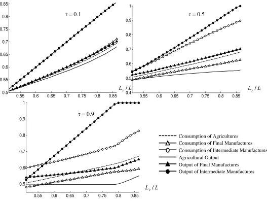
In the following part of this section, I will do the numerical analysis. I can get the results

shown in Figure 5 by using the same parameters used in section 3.1. With mobile capital,

I can see that whenτ =0.1, the varieties increasing effect is stronger than comparative

advantage effect, thus country y is net importer of intermediate manufactures and a net

exporter of agricultural products. But when trading cost decreases and τ =0.9, country y

larger market in intermediate manufactures and disproportionately larger share of

intermediate manufacturing production. Based on the same set of simulations, Figure 6

shows that country y's shares of nominal income are still smaller than its corresponding

shares of labor. However, country y's share of real income is higher than its share of

nominal income. And the higher the trading cost is, the higher country y's share of real

income is. Combining the simulation results in section 3.1 and 3.2, it indicates that trade

increases the real per capita income difference between the two countries while capital

mobility alleviates it. Therefore, liberalization of capital mobility can help reduce income

inequality across countries.

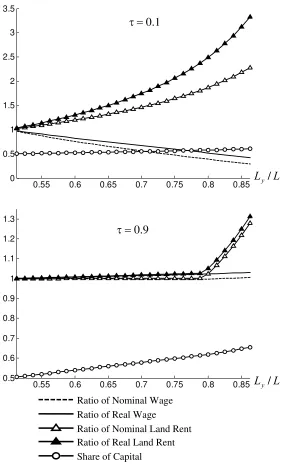
In Figure 7, I decompose income into factor returns again. I can see that both

country y's nominal and real land rents are higher than those of country x's. When trading

cost is high (τ =0.1) and there is not much trade, both nominal and real wage ratios are

smaller than 1, i.e., both country y's nominal and real wages are lower than those of

country x's. The difference increases in labor concentration in country y. This result is

similar with the case in section 3.1. However, when trading cost is low (e.g., τ =0.9) and

trade increases, the ratio of real wage becomes higher than 1 and the factor return

differences between the two countries are much smaller than those in Figure 3. I can also

see that the share of capital used by country y increases in country y's labor share and

value of τ . It means that both the increase of trade between the two countries and the

increase of labor concentration help country y attract more capital. This can be explained

intuitively. Without capital mobility, due to the abundant labor endowment, country y has

lower labor cost, and cheaper intermediate manufacturing input than country x. Once the

manufactures attracts capital from country x. On the other hand, the lower trading costs

can further decrease country y’s intermediate manufacturing cost and increase the capital

inflow. The inflow of capital increases country y's marginal product of labor, which

offsets the decrease of country y's marginal product of labor due to the increase of labor.

Therefore, I see that country y's real wage is higher than that of country x's. These results

can be summarized in the following proposition:

Proposition 5. Based on our simulation, when capital is mobile across countries,

production concentration caused by the vertical linkage of industries occurs. The capital

mobility also reduces the wage gap exists between the two countries due to the labor

endowment differences.

3.3.The Two-Country Model with Transportation Cost for All Sectors

A very important assumption for the above NEG models is that only trade of

differentiated goods involves trade costs. But empirical work [Rauch (1996), HelliIll

(1995), McCallum (1995), Harrigan (1993) and Ii (1996)] shows that conventional trade

costs are higher for homogeneous goods than for differentiated goods. Davis (1998) finds

that the transportation assumption is crucial to Krugman's CP model and unless the trade

cost is unusually higher for differentiated goods (more than 28 times of homogeneous

goods’ trade cost), each economy will remain in the proportional equilibrium.

In this section, I examine the robustness of my model by assuming agriculture has

the same trade cost as manufactures.

Assume that all conditions stay the same as in section 3.2, except that agriculture

now has the same trade cost as manufactures. Use the price of agricultural products in

Ay Ax Ay

y y y y y y x x x x x

x X X

P

K r L w w g A K r L w w g

A _⎟⎟= +

⎠ ⎞ ⎜

⎜ ⎝

⎛ + +

+ + +

− ) ( ) ( )

1

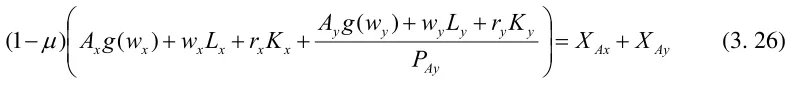
( μ (3. 26)

Equations of w_x, w_y, r_xand r_ycan be derived through the nonlinear equation system (3.

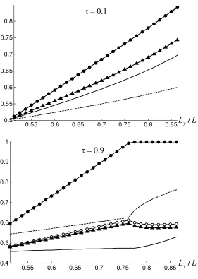
19), (3. 20), (3. 24) and (3. 26). Figure 8 and Figure 9 display our simulation results.

When τ =0.1, I can see that Figure 8 is quite similar to Figure 7. However, when τ =0.9,

Figure 9 shows that the ratio of real wage becomes much greater than 1. When country

y's share of labor is greater than 0.77, country x stops producing intermediate

manufactures and the country y's real wage increases dramatically relative to that of

country x's. This can be explained by the involvement of trade costs for agricultures.

Country y's labor endowment is so abundant that it has absolute advantages in both

manufacture and agricultural sectors. But its comparative advantage is still in the

manufactures sector. Therefore, it is a net exporter of intermediate manufactures and net

importer of agricultural products when trading cost is very low (τ =0.9). In this situation,

the involvement of trading costs for agricultural products will increase the price of

country x's exports, i.e., agricultural products, thus decrease its comparative advantage in

that sector and its gain from trade. This will further decrease country x's factor returns,

including real wage. Therefore, the involvement of trading costs for agricultural products

increases the gap of real wage between the two countries from another direction. It

increases the relative real wage of country y, which has comparative advantage in the

manufactures sector. In other words, the involvement of trading costs for agricultural

Proposition 6. Based on the simulations, when there are trade costs for agricultural

products, the agglomeration effect in manufacturing increases and capital mobility still

can help reduce the inequality across countries.

4. Conclusions

This paper studies how the existence of economies of scale and the trading cost

affect the industrial distribution，the trade pattern and the wage difference of two

countries. I set up a two-country general equilibrium model by incorporating a capital

factor into the NEG model. I simulate the effects of capital mobility and diminishing

marginal returns on the economy. Based on Davis (1998)'s comments on Krugman's CP

model, I also check the robustness of my results to the introduction of trade costs for

agricultural goods.

From the numerical simulation, I find that agglomeration of labor-intensive

industries occurs in the labor-abundant country if the trading cost is sufficiently low. The

agglomeration occurs regardless of whether or not there are trading costs for agriculture

and capital mobility across countries. But a larger market does not necessarily have a

disproportionately larger share of production in all industries as previous NEG models

predicted. The effect of comparative advantage impedes the agglomeration of industries

when the country with a smaller market has the comparative advantage in the same

industries. This is consistent with Ricci (1999)'s conclusion that the agglomeration effect

weakens the specialization degree. On the other hand, when comparative advantage is not

sufficiently strong and trading cost is high, the varieties increasing effect can also impede

In the case of immobile capital, trade occurs when comparative advantage is

sufficiently strong to compensate for the trade cost and both countries gain from trade.

There is a gap between the two countries’ wages in both nominal and real terms. Both

nominal and real wages are lower in the labor abundant country. This is caused by the

endowment difference and the existence of trading costs. The gap is reduced by trade, but

still increases in the labor endowment difference due to the effect of diminishing

marginal returns. This result differs from most previous NEG models’ simulation results

which show that the wage level is higher in the labor abundant country when the trading

cost is sufficiently low. This is because those models do not have capital as an input in

manufacturing production. They do not reflect the effect of diminishing marginal returns

of labor.

My simulation results show that capital mobility narrows the wage (either

nominal or real) difference across countries. The real wage in the labor abundant country

is even slightly higher than that in the other country when the trading cost is sufficiently

low. When both mobile capital and agricultural trade costs are involved in the model, the

simulation results show that the countries with abundant labor have much higher real

wage than the other country. This suggests that for the country with strict capital controls,

capital liberalization can help reduce wage difference between countries in both nominal

and real terms.

The simulation results of this paper indicate that with economies of scale

technology and labor immobile across countries, as long as the trade pattern follows what

comparative advantages indicate, low trading costs will not cause the catastrophic

This is because of the involvement of capital as a variable input in the final

manufacturing production. By introducing capital, I have completely ruled out the

demand and cost linkage associated with the labor-involved production from the

capital-intensive industry. As a result, only the labor-capital-intensive industries agglomerate into the

labor abundant countries. The catastrophic agglomeration does not happen in the

capital-intensive industries. This is different from other capital-involved NEG models which

have capital as a fixed input for the intermediate manufactures and still get the

catastrophic agglomeration for all industries. At the same time, the inclusion of both

labor and capital as variable manufacturing inputs enables the model to reflect the effects

of comparative advantages and the diminishing marginal returns to labor and capital,

which work to counter to the agglomeration effect. The simulation results show that when

labor is not the only variable input in manufacturing production, the labor abundant

country does not necessarily have a higher wage rate as other NEG models predict.

With labor immobile across countries, my model predicts that capital mobility

will increase the return to labor in the labor abundant region relative to the other region.

However, labor is more likely to be mobile across sub-regions within a country. How will

labor mobility together with capital mobility affect an economy? This is an important

REFERENCES

Amiti, Mary, 2005. "Location of vertically linked industries: agglomeration versus

comparative advantage," European Economic Review, Elsevier, vol. 49(4), pages

809-832.

Baldwin, Richard E., 1999. “Agglomeration and endogenous capital.” European

Economic Review, 43(2), 253-280.

Baldwin, R., R. Forslid, P. Martin, G. Ottaviano and F. Robert-Nicoud, 2003. Economic

Geography and Public Policy, Princeton University Press.

Davis, D.R. 1998 “The Home Market Effect, Trade and Industrial Structure.” American

Economic Review, 88(5), 1264-1276.

Dixit, Avinash K and Stiglitz, Joseph E, 1977. “Monopolistic Competition and Optimum

Product Diversity.” American Economic Review, 67(3), 297-308.

Ethier, Wilfred J, 1982. “National and International Returns to Scale in the Modern

Theory of International Trade.” American Economic Review, 72(3), 389-405.

Forslid, Rikard, 1999. “Agglomeration with Human and Physical Capital: an Analytically

Solvable Case.” CEPR Discussion Papers 2102, C.E.P.R. Discussion Papers

Fujita, Masahisa and Krugman, Paul and Venables, Anthony J. 1999. The spatial

economy : cities, regions and international trade. MIT Press, Cambridge, Mass..

Harris, C.D., 1954. “The market as a factor in the localization of industry in the United

States.” Annals of the Association of American Geographers, 44, 315– 348.

Henderson, J. V., and Thisse, J. 2004. Handbook of Regional and Urban Economics.

Krugman, Paul. 1991. “Increasing Returns and Economic Geography.” Journal of

Political Economy, 99(3), 483-99.

Martin, Philippe & Rogers, Carol Ann, 1995. “Industrial location and public

infrastructure,” Journal of International Economics, Elsevier, 39(3-4), 335-351.

Ottaviano, Gianmarco I P, 1996. “Monopolistic Competition, Trade, and Endogenous

Spatial Fluctuations.” CEPR Discussion Papers 1327, C.E.P.R. Discussion Papers.

Puga, D. 1999. “The Rise and Fall of Regional Inequalities.” Europe Economic Review,

43, 303-334

Ricci, Luca, 1999. “Economic geography and comparative advantage: Agglomeration

versus specialization,” European Economic Review, 43(2), 357-377

Venables, Anthony J, 1996. “Equilibrium Locations of Vertically Linked Industries.”

0.55 0.6 0.65 0.7 0.75 0.8 0.85 0.5

0.55 0.6 0.65 0.7 0.75 0.8 0.85

0.55 0.6 0.65 0.7 0.75 0.8 0.85 0.4

0.5 0.6 0.7 0.8 0.9 1

0.55 0.6 0.65 0.7 0.75 0.8 0.85

0.5 0.6 0.7 0.8 0.9 1

Figure 1. Trade Patterns of Two Countries with Immobile Factors

Consumption of Agricultures Consumption of Final Manufactures Consumption of Intermediate Manufactures Agricultural Output

Output of Final Manufactures Output of Intermediate Manufactures

1 . 0

=

τ τ=0.5

9 . 0

= τ

L

L_y/ L_y/L

0.55 0.6 0.65 0.7 0.75 0.8 0.85 0.5

0.55 0.6 0.65 0.7

0.55 0.6 0.65 0.7 0.75 0.8 0.85

0.5 0.55 0.6 0.65 0.7 0.75

0.55 0.6 0.65 0.7 0.75 0.8 0.85

0.5 0.55 0.6 0.65 0.7 0.75 0.8

Figure 2. Income Ratios of Two Countries with Immobile Factors

Share of Nominal Income

Share of Real Income

1 . 0

=

τ _τ=0.5

9 . 0

= τ

L

L_y/ L_y/L

0.55 0.6 0.65 0.7 0.75 0.8 0.85 0

0.5 1 1.5 2 2.5

0.55 0.6 0.65 0.7 0.75 0.8 0.85

0.5 1 1.5 2 2.5 3 3.5 4 4.5

0.55 0.6 0.65 0.7 0.75 0.8 0.85

0.5 1 1.5 2 2.5 3 3.5 4 4.5

Figure 3. Factor Returns of Two Countries with Immobile Factors

1 . 0

=

τ τ=0.5

L

Ly/ Ly/L

9 . 0

= τ

L L_y/

Ratio of Nominal Wage Ratio of Real Wage

Ratio of Nominal Land Rent Ratio of Real Land Rent

0.55 0.6 0.65 0.7 0.75 0.8 0.85 0

2 4 6 8 10 12 14 16

0.55 0.6 0.65 0.7 0.75 0.8 0.85

0 2 4 6 8 10 12 14 16

0.55 0.6 0.65 0.7 0.75 0.8 0.85 0

2 4 6 8 10 12 14 16 18

Figure 4. Output of Two Countries with Immobile Factors

Real Income

Final Manufactures Output Agricultural Output

L Ly/

9 . 0

= τ

1 . 0

=

τ τ=0.5

L

0.55 0.6 0.65 0.7 0.75 0.8 0.85 0.5

0.55 0.6 0.65 0.7 0.75 0.8

0.55 0.6 0.65 0.7 0.75 0.8 0.85 0.5

0.6 0.7 0.8 0.9 1

Figure 5. Trade Patterns of Two Countries with Mobile Capital and Immobile Labor Consumption of Agricultures

Consumption of Final Manufactures Consumption of Intermediate Manufactures Agricultural Output

Output of Final Manufactures Output of Intermediate Manufactures

1 . 0

= τ

L Ly/

9 . 0

= τ

0.55 0.6 0.65 0.7 0.75 0.8 0.85

0.5 0.55 0.6 0.65 0.7

0.55 0.6 0.65 0.7 0.75 0.8 0.85 0.5

0.52 0.54 0.56 0.58 0.6 0.62 0.64 0.66

Figure 6. Income of Two Countries with Mobile Capital and Immobile Labor Share of Nominal Income

Share of Real Income

1 . 0

= τ

L L_y/

9 . 0

= τ

0.55 0.6 0.65 0.7 0.75 0.8 0.85 0

0.5 1 1.5 2 2.5 3 3.5

0.55 0.6 0.65 0.7 0.75 0.8 0.85 0.5

0.6 0.7 0.8 0.9 1 1.1 1.2 1.3

Figure 7. Factor Returns of Two Countries with Mobile Capital and Immobile Labor Ratio of Nominal Wage

Ratio of Real Wage

Ratio of Nominal Land Rent Ratio of Real Land Rent Share of Capital

L Ly/

L Ly/

9 . 0

= τ

1 . 0

0.55 0.6 0.65 0.7 0.75 0.8 0.85 0

0.5 1 1.5 2 2.5 3 3.5

0.55 0.6 0.65 0.7 0.75 0.8 0.85 0.5

1 1.5

Figure 8. Factor Returns of Two Countries with Transportation Cost for All Sectors Ratio of Nominal Wage

Ratio of Real Wage

Ratio of Nominal Land Rent Ratio of Real Land Rent Share of Capital

1 . 0

= τ

L Ly/

9 . 0

= τ

0.55 0.6 0.65 0.7 0.75 0.8 0.85 0.5

0.55 0.6 0.65 0.7 0.75 0.8

0.55 0.6 0.65 0.7 0.75 0.8 0.85 0.4

0.5 0.6 0.7 0.8 0.9 1

Figure 9. Trade Patterns of Two Countries with Transportation Cost for All Sectors Consumption of Agricultures

Consumption of Final Manufactures Consumption of Intermediate Manufactures Agricultural Output

Output of Final Manufactures Output of Intermediate Manufactures

9 . 0

= τ

L Ly/

1 . 0

= τ