Munich Personal RePEc Archive
A local dynamic conditional correlation
model
Feng, Yuanhua
Maxwell Institute for Mathematical Sciences, Heriot-Watt University
2006
Online at
https://mpra.ub.uni-muenchen.de/1592/
A Local Dynamic Conditional Correlation Model
Yuanhua Feng
Department of Actuarial Mathematics and Statistics
Heriot-Watt University
Abstract: This paper introduces the idea that the variances or correlations in financial
returns may all change conditionally and slowly over time. A multi-step local dynamic
conditional correlation model is proposed for simultaneously modelling these components. In particular, the local and conditional correlations are jointly estimated by multivariate kernel
regression. A multivariate k-NN method with variable bandwidths is developed to solve the
curse of dimension problem. Asymptotic properties of the estimators are discussed in detail. Practical performance of the model is illustrated by applications to foreign exchange rates.
JEL Classification Codes: C32, G0, G1
Key Words: Local and conditional correlations, multivariate nonparametric ARCH,
mul-tivariate kernel regression, mulmul-tivariate k-NN method.
1
Introduction
Financial econometrics becomes an active new discipline of economics (Engle, 2001) with one of its main focuses on the development of new tools for estimating and forecasting dynamic
variances and correlations of financial assets. In the seminal paper Engle (1982) the ARCH
(autoregressive conditional heteroskedasticity) model is introduced for modelling conditional
variances, which is then generalized by Bollerslev (1986) to the GARCH (generalized ARCH) model. See Bollerslev et al. (1992) for an earlier survey on these models. For modelling
dynamic correlations some multivariate GARCH (MGARCH) models with complex
param-eter specification, e.g. the vec-model (Bollerslev et al., 1988) and the BEKK (Engle and Kroner, 1995) are first introduced. A simple MGARCH, called the constant conditional
cor-relation (CCC) model, was introduced by Bollerslev (1990), where the conditional variances
are modelled by separate univariate GARCH models under constant correlation assumption.
∗Dr. Yuanhua Feng, Department of Actuarial Mathematics and Statistics, Heriot-Watt University, EH14
Recent research on these topics focuses on developing approaches with dynamic
correla-tions and simple parameter specification so that the models are applicable to many assets. The well known proposal is the dynamic conditional correlation (DCC) model introduced
by Engle (2002) (see also Engle and Sheppard, 2001). A similar approach is proposed by
Tse and Tsui (2002). The DCC model is generalized by Cappiello et al. (2003) and Hafner and Franses (2003) to allow for richer correlation dynamics. Pelletier (2006) extended the
CCC model to a regime-switching conditional correlation model, where the correlation
ma-trix is constant within a regime but different across regimes. Silvennoinen and Ter¨asvirta (2005) extended this idea to a smooth-transition conditional correlation model by allowing
for smooth change in the conditional correlations between two extreme states according to
some transition function. Most recently, Hafner et al. (2005) introduced a semiparametric generalization of the CCC model, where conditional correlations are estimated by a
univari-ate kernel regression. For more information on the development of MGARCH models we
refer the reader to the recent review of Bauwens et al. (2005) and references therein.
In this paper cases with simultaneous smooth local changes and conditional dynamics
in variances and correlations are considered are considered. A local dynamic conditional correlation (LDCC) model is introduced for all of these components, where mooth change in
the mean of financial returns is also allowed. The variances are decomposed into a conditional
and a local (unconditional) parts. The correlation structures are jointly modelled by a
multivariate nonparametric ARCH-type approach with the observation time and some other variables based on past observations as regressors. The order of such a model does not depend
on the number of assets. The LDCC model is hence applicable to cases with a large number of
assets. The proposal is motivated by the observation that financial market conditions often change slowly which in turn causes slowly changing components in asset returns. Proper
estimation of these quantities will improve the estimation of further parametric models and
then improve the forecasting of future trends, variances and correlations. Modelling of conditional and local variances in univariate financial returns is studied by Feng (2004)
under a semiparametric GARCH model. Most recently, Feng and Yu (2005) and Herzel et
al. (2006) investigated the slowly changing variances and correlations in financial returns under a multivariate random walk model and a VAR(1) model respectively. To our knowledge
multivariate models with both conditional and slowly changing unconditional correlations is
not yet studied in the literature.
A multi-step semiparametric procedure is proposed for estimating the LDCC model. The
ap-proaches. Conditional variances are then estimated from the standardised observations using
separate univariate GARCH models. A multivariate kernel regression is proposed for jointly estimating the local and conditional correlations. This idea can also be applied to time series
smoothing involving common exogenous variables. Ak-NN (k-nearest-neighbours) method is
developed to solve the curse of dimension problem in multivariate nonparametric regression, which allows for automatic adaptation of the bandwidth to the design density. Asymptotic
properties of the proposed estimators are discussed in detail. The use of causal smoothing
technique is also investigated briefly. Practical performance of the proposal is illustrated by applications to several foreign exchange rate series. The idea to estimate and remove the
slowly changing variances applies to any MGARCH model. Semiparametric generalizations
of the CCC and DCC models are given as examples.
The paper is organized as follows. The model is defined in the next section. Section 3 describes the step-wise semiparametric estimation procedure. Asymptotic properties of the
proposed estimators of the local and conditional correlations are investigated in Section 4.
In Section 5 the model is applied to data examples. Final remarks in Section 6 concludes the paper. Some auxiliary results and proofs of theorems are given in the appendix.
2
The models
In this section we first define the semiparametric LDCC model. Related semiparametric extensions of the CCC and DCC models are then described.
2.1
The main approach
Let Xt, t = 1,2, ..., n, be a vector return series of d financial assets, which are assumed to
follow the nonparametric conditional heteroskedastic model
Xt =µ(τt) +rt∗, (1)
where τt=t/ndenotes the re-scaled time, µ(·) is the nonparametric local mean vector and
rt∗|Ft−1 ∼N(0,Σt), (2)
whereFt−1 denotes the information set generated by past observations and the location, and
Σt is the total covariance matrix. It is proposed to decompose Σt as follows.
where DL
t = diag(σi(τt)), DtC = diag(
√
hit) and Rt = (ρijt), i, j = 1, ..., d, where σi2(·) are
the local variances, hit are the conditional variances and ρijt are the dynamic correlations
which may depend on both the location and past observations. Furthermore, it is assume
that E(DC
t ) = Id with Id denoting the identity matrix, so that (3) is uniquely defined. Let
Dt = DLtDtC = diag(σi(τt)√hit) which is the total standard deviation matrix. The total
covariance matrix is decomposed into a conditional and an unconditional components. The
latter depends on the middle-term market conditions and often changes smoothly. The
process defined by (1) to (3) is non-stationary. Following Dahlhaus (1997) it can be shown that such a process is jointly locally stationary under suitable conditions.
The local variance σ2
i(·) can be easily estimated by nonparametric regression. Let rt =
(DL
t)−1rt∗ be the standardized observations. Following the CCC and DCC, the conditional
variances can be modelled by univariate GARCH models,
hit =αi0+
pi X
l=1
αilr2i(t−l)+
qi X
m=1
βimhi(t−m), (4)
where αi0 > 0, αil, βim ≥ 0 and Ppil=1αil +Pqim=1βim < 1. The orders pi and qi of the
GARCH models may different for different assets.
Now letǫt= (DtC)−1rt, where ǫt∼N(0, Rt). Unlike the diagonal variance matrix, it is not
easy to decompose Rt into a local and a conditional parts separately. We will propose to
estimate the local and conditional dynamics in Rt jointly in a nonparametric way. Consider
the conditional influence of p lagged observations. A nonparametric regression with ǫt−j,
j = 1, ..., p, as regressors is not relevant in practice, because such a model cannot be applied
to a large number of assets. In this paper some univariate random variablesyjt as functions
of ǫt−j, j = 1, ..., p, which summarize the effect of ǫt−jǫ′t−j on the correlation dynamics, will
be used as regressors, where p > 0 is the order of the model which does not depend on the
number of assets. This makes the model applicable to a multivariate time series with many
components. Let and yt = (y1t, ..., ypt)′. In the LDCC model defined in the following the
local and conditional correlation matrix will be denoted by R(τt;yt) = (ρij(τt;yt)) instead
of by Rt. The proposed model is defined by
R(τt;yt) =g(τt;yt), (5)
where g(·) is a smooth function. A model defined by (1) through (5) will be called a
model (see later). Another closely related model is the semiparametric dynamic correlation
model most recently proposed by Hafner et al. (2005), whereR(·) is assumed to be a smooth
function of a univariate observable variable. If some exogenous variables, e.g. returns of some
other financial index are introduced into the LDCC model, we will obtain local extensions
of the model in Hafner et al. (2005). A nonparametric GARCH is proposed by B¨uhlmann
and McNeil (2002). It is worthwhile to introduce the latent variables R(τt−i;·), i= 1, ..., q,
into (5) to extend the LDCC to a multivariate nonparametric GARCH-type model.
2.2
Combination with other models
The first part of the proposed model can be used to obtain semiparametric generalizations
of well known approaches in the literature. Extensions of the CCC and the DCC models
following this idea will be discussed here briefly. If it is assumed that the changes in the correlations only depend on the location but not on the past observations, we will have
Rt = R(τt), which can be simply estimated from ǫt using nonparametric regression. Now,
we obtain a generalized CCC model with slowly changing variances and correlations which
is also a LDCC(0) model.
On the other hand, if it is assumed that the unconditional correlation matrix is constant,
i.e. Rt only depends on the past observations but not on the location, we will obtain another
simplified case. Now, Rt can be modelled by a parametric MGARCH model. For instance,
following the DCC model Rt can be modelled by
Rt = (diag(Qt))−1/2Qt (diag(Qt))−1/2,
Qt = 1−
L X
l=1
αl−
M X
m=1
βm
!
¯
R+
L X
l=1
αl(ǫt−lǫ
′
t−l) + M X
m=1
βmQt−m, (6)
where αl, βm ≥ 0, PLl=1αl +PMm=1βm < 1 and ¯R is the constant correlation matrix of
ǫt. Equations (1) through (4) and (6) define a DCC model with slowly changing variances
which is however not a special case of the LDCC model. Such a model can be estimated by
combining the first stage of the algorithm proposed in the next section and the second stage
of that in Engle and Sheppard (2001). Moreover, ifRt is assumed to follow (2.4) in Pelletier
(2006) or (7) in Silvennoinen and Ter¨asvirta (2005) we will obtain corresponding extensions
3
The estimation
The LDCC model can be estimated using a step-wise procedure. The first stage of the
procedure consists of some common non- and semiparametric estimators which applies to
other MGARCH models. The second stage is a multivariate kernel regression for estimating R(·).
3.1
Estimating the means and the variances
Letxt, t= 0,1, ..., n, denote the observations and xit, i= 1, ..., d, thei-th element ofxt. Let
Kµi(u) be a kernel function andbµi the bandwidth. Thenµi(τ), the i-th element ofµ(τ) can
be estimated by solving the local linear regression problem
(ˆa0,aˆ1)′ = arg min
a0,a1
n X
t=1
(xit−a0−a1(τt−τ)2Kµi
τt−τ
bµi
. (7)
We have ˆµi(τ) = ˆa0. Now let ˆµ(τt) = (ˆµ1(τt), ...,µˆd(τt))′ and ˆr∗t = xt −µˆ(τt) denote the
residuals. Denote by V(τ) = (σ2
1(τ), ..., σd2(τ))′ the vector of the local variances. Let KVi(u)
be another kernel and bVi another bandwidth. It is proposed to estimate the local variances
using a kernel estimator to ensure that ˆσi(τ)>0 a.s. (almost sure). Related proposals may
be found e.g. in Fan and Yao (1998), Feng and Heiler (1998) and H¨ardle et al. (1998). We
define
ˆ σ2i(τ) =
n P t=1
KVi
τt−τ
bVi
(ˆr∗
it)2 n
P t=1
KVi
τt−τ
bVi
(8)
and set ˆV(τ) = (ˆσ2
1(τ), ...,σˆd2(τ))′. IfR(·) only depends on the location, the local covariances
σij, say, can be analogously estimated from ˆrit∗ and ˆr∗jt. Then ρij(τ) can be estimated by
ˆ
ρij(τ) = σiˆ σij(ˆτ)ˆσj(τ)(τ).
By means of ˆV we obtain the standardized residuals ˆrit= ˆr∗it/σˆi(τt). ˆrithave asymptotically
constant variance. Let θi = (αi0, αi1, ..., αipi, βi1, ..., βiqi)′. The unknown parameter vector θi
can be estimated from ˆrit, t = 1, ..., n, using some standard software for fitting a univariate
GARCH model. Then we will obtain ˆDC
t . Let ˆrt = (ˆr1t, ...,rˆdt)′and ˆǫt = ( ˆDCt )−1rˆt. Assuming
constant unconditional correlations,Rt can be now estimated from ˆǫt following equations (7)
3.2
A multivariate
k
-NN kernel approach for
R
(
·
)
Now, consider the estimation of R(·) in a LDCC(p) model with p > 0. In this paper the
regressors yjt for j = 1, ..., p and t=p+ 1, ..., n are defined by
yjt= 1I′ǫt−jǫ′t−j1I, (9)
where 1I is a vector of d ones. Note that yjt = (ǫ1(t−j) +... +ǫd(t−j))2 ≥ 0. It is well
known that even in one-dimensional nonparametric regression for financial data we will be
faced by the problem of data sparsity. In the current case this problem arises together with the curse of dimension. Now, the use of fixed bandwidths is not suitable. To improve
the theoretical and practical performance of the proposed estimator and to ensure that the
computer program will run smoothly without any numerical problem, a local multivariatek
-NN method is developed. Consider the estimation ofR(·) atτ andy= (y1, ..., yp)′. Following
this algorithm the bandwidth b for yj, j = 1, ..., p, will adapt automatically to the design
density. Let t0 = [nτ] and assume that t0 > p, where [x] denote the largest integer which is
smaller than x. Letk be a chosen integer such thatk → ∞and k/n→0, as n→ ∞. Letb0
be the half bandwidth for the re-scaled time such thatb0 →0,nb0 → ∞ and (nb0)−1k→0,
as n→ ∞. Here b0 and k are two smoothing parameters chosen beforehand. Let k1 = [nb0]
and k0 = 2k1+ 1. k0 is the total number of observations involved. The bandwidth used for
yj is defined in the following way.
1. Let n1 = t0 −k1 and n2 = t0 +k1, if t0 ≥ k1 +p, or n1 = p+ 1 and n2 = p+k0,
otherwise.
2. Let dt= [(yt−y)′(yt−y)]1/2 denote the Euclidean distance between yt and y.
3. Orderdtstarting with the smallest value and define the bandwidthbforyj,j = 1, ..., p,
to be the k-th ordered dt.
Following this algorithm alwaysk observations will be selected fromk0 observations around
t0, independently ofpand the design density. The bandwidthb0 is chosen separately
before-hand, because τ is of a different scale than yj. To simplify the algorithm, kernel functions
forτ andyj are also chosen separately. LetK0(v) be a univariate kernel with support [−1,1]
and u = (u1, ..., up)′ a p-dimensional spherical kernel defined on the unit ball. Then the
finally used kernel is the product of K0(v) and K(u). The proposed estimator is defined by
ˆ
with the matrix-wise multivariate kernel estimator
ˆ
Q(τ;y) =
n2
P t=n1
K0
τt−τ
b0
K y1t−y1
b , ...,
ypt−yp b
ˆ ǫtˆǫ′t
n2
P t=n1
K0
τt−τ
b0
K y1t−y1
b , ...,
ypt−yp b
(11)
=:
n2
X
t=n1
wtˆǫtˆǫ′t,
where n1 and n2 are defined before. The entries of ˆR(·) will be denoted by ˆρij(·) and those
of ˆQ(·) by ˆqij(·). The weights wt are determined by the kernels, b0, k as well as the past
observations ǫt−1, ...,ǫt−p, and are non-zero for the selected observations and zero otherwise.
The curse of dimension problem is solved and a LDCC model of higher order can be easily
fitted. In the above approach wt are the same for all entries of ˆQ(·). This ensures that
ˆ
Q(·) is a.s. positive semidefinite, because now it is a Gram matrix, and ˆR(·) is hence a.s.
a correlation matrix. The derivation of the covariances between ˆqij(·) and ˆqlm(·) is also
simplified due to the use of same weights for both.
Remark 1. In practice a causal smoother involving only past observations might be prefer-able. Setting n1 = t−k0 and n2 = t−1 for t > k0 +p in Step 1 of the k-NN algorithm
we will obtain a causal estimator of R(·) which will also be applied to the data examples in Section 5.
4
Main results
Both ˆQ(·) and ˆR(·) are estimators of R(·) which have similar properties. However, ˆR(·) is a
correlation matrix but ˆQ(·) is usually not. In the following the asymptotic properties of ˆQ(·)
will be first investigated. Properties of ˆR(·) are then derived based on those of ˆQ(·). Most
properties of ˆµ(·), ˆV(·) as well as ˆθ are known in the literature. The effect of the errors in
these estimators on ˆQ(·) will be discussed in the appendix. For the proof of the results the
following assumptions are required.
A1. i) The local mean and variance functions µi(·) and Vi(·), i= 1, ..., d, are at least twice
continuously differentiable. ii) The kernels Kµi and KVi for estimating µ and V are all
symmetric densities with support [−1,1]. And iii) The estimators ˆµ and ˆV are obtained
A2. There exists a constant δ >0 such that E(r4+it δ)<∞ for each of the GARCH models
defined in (4).
A3. The estimation point (τ;y) is a multivariate interior point with τ ∈ (0,1) and yj >0
for all j = 1, ..., p.
A4. Assume that ǫt ∼N(0, R(τt;yt)) and ǫt and ǫs are independent fort 6=s.
A5. R(τ;y) is positive definite, uniformly inτ and y, whose off-diagonal entries are at least
twice continuously differentiable with respect to τ ∈[0,1] andy on their support.
A6. The kernelK0is a symmetric density defined on [−1,1] with
R
v2K
0(v)dv =µ2(K0)>0.
The spherical kernel K is a density defined on the unit ball such that R
uK(u)du = 0 and
R
uiujK(u)du=δijµ2(K) with µ2(K)>0.
A7. i) The bandwidth b0 is of higher order than n−1/5, denoted by b0 > O(n−1/5). ii) b0
satisfies b0 →0, nbp0+1 → ∞ asn → ∞. And iii)k is chosen by k =Cknbp0+1 with Ck>0.
A1 summarizes the common conditions on the estimators ˆµ(·), ˆV(·) as well as ˆθin the first
stage, which together with A7 i) ensures that the effect of the errors in these estimators are
asymptotically negligible and hence ˆQ(·) and ˆR(·) obtained from ˆǫtor from the unobservable
ǫt have the same asymptotic properties. A2 is required for the asymptotic normality of ˆVi(·)
and the resulting ˆθi. Necessary and sufficient conditions that guarantee this may be found
e.g. in Ling and McAleer (2002), and in Bollerslev (1986) for GARCH(1, 1) models. Note
that E(rit4+δ)<∞ impliesPpil=1αil+Pqim=1βim<1 as assumed before. A3 is introduced to
avoid the boundary effect in the time dimension which simplifies the proofs. In the appendix
it will be explained that there is indeed no boundary effect caused by the regressors yj. A4 is
not a necessary condition which can be replaced by suitable assumptions on the distribution
of ǫt (see Hafner et al., 2005). A5, A6 and A7 ii) are regularity conditions in multivariate
nonparametric regression. A5 also ensures that the off-diagonal elements ofR(·) are strictly
between -1 and 1, uniformly in τ and y.
A7 ii) and iii) ensure that the bandwidth b for the regressors yj obtained by the k-NN
method is of the same order of magnitude as b0. This is given by the following lemma.
Lemma 1. Assume that y is observable with continuous density on its support and that
0< f(x)<∞ in a neighbourhood ofy. Then under A7 ii) and iii) the bandwidth b obtained
by the k-NN method is given by
b =. C0b0 with C0 =
Ck
2
Γ(p/2 + 1)
πp/2f(y)
1/p
Lemma 1 is given under common regularity conditions on the design density which provides
a basis for extending the main results in this paper to more general cases. The explicit
form of f(y) under A4 will be given in the appendix. A3 and A4 together ensure that the
conditions of Lemma 1 hold. It is clear that Lemma 1 remains to be true whenyis estimated
consistently.
Now, let ξlmt = ǫltǫmt, l, m = 1, ..., d. Then we have ρlm(τt;yt) = E[ξlmt|y = yt]. Let
γ2
lm denote the conditional variance of ξlmt and γlm,rs the conditional covariance between
ξlmt and ξrst. Let R(K0) =
R
K2
0(v)dv and R(K) =
R
K2(u)du. Let ▽
f(y) and ▽lm(y)
denote the two p×1 vectors of the gradient of f(y) and ρlm(τ;y) respectively w.r.t. y,
and let Hlm(τ;y) denote the (p+ 1)× (p+ 1) Hessian matrix of ρlm(τ;y). Finally, let
T = diag(µ2(K0)/µ2(K), C02, ..., C02), Clm = 12tr{Hlm(τ;y)T + 2C02 ▽f (y)▽lm (y)′/f(y)}
and CV = 2∗πp/2/Γ(p/2 + 1)R(K0)R(K). Note that Clm depends on τ and y. Then the
following holds.
Theorem 1. Under Assumptions A1 to A7 we have
i) Bias[ˆqlm(τ;y)]=. Clmµ2(K)b20, for l 6=m,
ii) Bias[ˆqlm(τ;y)] =O[b2Vl+ (nbVl)−1] =o(b20), forl =m,
iii) var[ˆqlm(τ;y)]=. CVk−1γlm2 and
iv) cov[ˆqlm(τ;y),qˆrs(τ;y)]=. CVk−1γlm,rs.
The regressors τ and y have slightly different effects on the asymptotic results, because
the used bandwidths for them are different and that τt are equidistant. For fixed k the
asymptotic variances and covariances of the proposed estimators do not depend on the
design density. But the asymptotic biases depend on f(y) through the constant C0. If Ck
is fixed, the optimal b0, which minimizes the dominating part of the MSE (mean squared
error) of ˆqlm(τt;y), is given by
bopt0 =Coptn−
1
p+5 with C
opt=
(p+ 1)CVγlm2
4C2
lmµ22(K)Ck p+51
. (13)
The optimal order of the MSE isO(n−p+54 ). Note that the use of a fixedC
kis only suboptimal.
The optimal choice of Ck so that the constant of the dominating part of the MSE is also
minimized and the data-driven selection ofbopt0 will be discussed elsewhere.
Similar results hold for ˆρlm(·). In particular they are also asymptotically normal. Consider
Theorem 2. Assume that b0 = Cbn−
1
p+5 and that C
b, Ck > 0 are two positive constants.
Then under the other conditions of Theorem 1 we have
√
k ρˆlm(τ;y)−ρlm(τ;y)
ˆ
ρrs(τ;y)−ρrs(τ;y) !
D
−→N
(
Cµ
Clm
Crs
!
, CV
γ2
lm γlm,rs
γlm,rs γ2rs !)
, (14)
where Cµ =µ2(K)Ck1/2C
(p+5)/2
b is an unknown constant and CV is as defined before.
If a bandwidth b0 =o(n−1/(p+5)) is used then the bias in ˆqlm(·) is asymptotically negligible.
Now Theorem 2 holds withCµbeing replaced by 0. Results in this case are useful for carrying
out confidence intervals of ρlm(·) (Hafner et al., 2005).
Remark 2. Similar asymptotic properties of the causal estimator described in Remark 1 can be obtained by setting τ = 1. This will not be discussed here in detail.
5
Applications
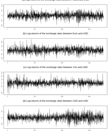
In the following the practical performance of the model is shown by applications to the daily foreign exchange rate series of the British Pound (Pound), Euro, Japanese Yen (Yen) and
Canadian Dollar (CAD) w.r.t. the US Dollar (USD) from 4 Jan 1999 to 30 December 2005.
The log-returns of these series are shown in Figure 1. The programmes are developed in S-Plus, which can also be run under R. In all of the examples corresponding univariate and
spherical Epanechnikov kernels are used. The nonparametric trend in the returns are fitted
using the SEMIFAR (semiparametric fractional autoregressive) model (Beran and Feng, 2002), where the bandwidths are automatically selected and it is also shown that the returns
are about uncorrelated, one of the properties of a GARCH process. The local variances
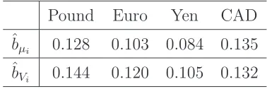
are then estimated from the corresponding residual series using bandwidths selected by the algorithm in Feng (2004). Table 1 lists the bandwidths for estimating the means and the
variances selected by these programmes. The estimated local means and local standard
deviations are omitted to save space.
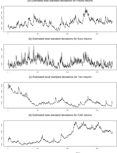
GARCH models are then fitted from the standardized residuals using S+GARCH. GARCH(1, 1) models are selected following the BIC for Pound, Yen as well as CAD. The fitted GARCH
models for the Euro returns of lower orders have however negative coefficients, for which a
GARCH(2, 2) model is hence used. The estimated conditional variances for each series are:
ˆ
Table 1. Selected bandwidths for ˆµi, ˆσi
Pound Euro Yen CAD
ˆbµi 0.128 0.103 0.084 0.135
ˆ
bVi 0.144 0.120 0.105 0.132
ˆ
h2t= 0.0980 + 0.1000ˆr2(2t−1)+ 0.0010ˆr22(t−2) + 0.7999ˆh2(t−2)+ 0.0101ˆh2(t−1),
ˆ
h3t= 0.0590 + 0.0139ˆr23(t−1)+ 0.9265ˆh3(t−1),
ˆ
h4t= 0.0360 + 0.0219ˆr24(t−1)+ 0.9415ˆh4(t−1).
The estimated total standard variations ˆσi(τt)·
p
ˆ
hitfor the return series are shown in Figure
2.
Selection of the smoothing parameters and the order of the LDCC model is still an open question. For a comparison, results using different parameter combinations will be given.
We will see that estimates using b0 andk within a large range have quite similar conditional
patterns. This means that the fitted results discover the nature of the true correlation
dynamics and the proposed model works well in practice. Note that for a LDCC(p) model
relatively large smoothing parameters should be used, because it is a (p+ 1)-dimensional
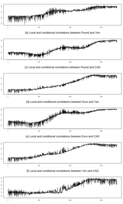
nonparametric regression. Figure 3 displays the estimated local and conditional correlations
of a LDCC(4) model with b0 = 0.18 andk = 400, i.e. Q(·) is estimated by 400 observations
selected from a total of 36% of all observations around t. Figure 4 shows the estimation
results of a LDCC(6) model with the same smoothing parameters.
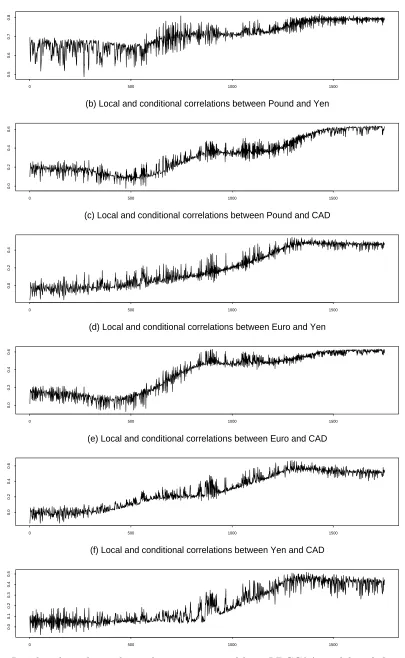
We see both the conditional and local changes are clear. The conditional effect changes
from one point to another. Information in the past observations may cause lower or higher
correlations comparing to the average level. Sometimes the conditional effect may cause clear changes in the correlations in both directions. The largest conditional changes in
correlations are as high as about 0.2. The average level of the correlations depends on the
location, which changes clearly in some periods. This also depends on the two series involved. For instance, the local change of the correlations between Pound and Euro is quite small,
because these two series are always highly correlated. An interesting phenomenon is that the
correlations between CAD and the other currencies were about zero at the beginning, but increase to about 0.5 at the end of the observation period. Note that the conditional changes
regressors yj are non-smooth over time. This fact can be also found from the examples
in Hafner et al. (2005). By comparing Figures 3 and 4 we can find that the LDCC(6) model seems to perform better than the LDCC(4). This observation provides evidence for
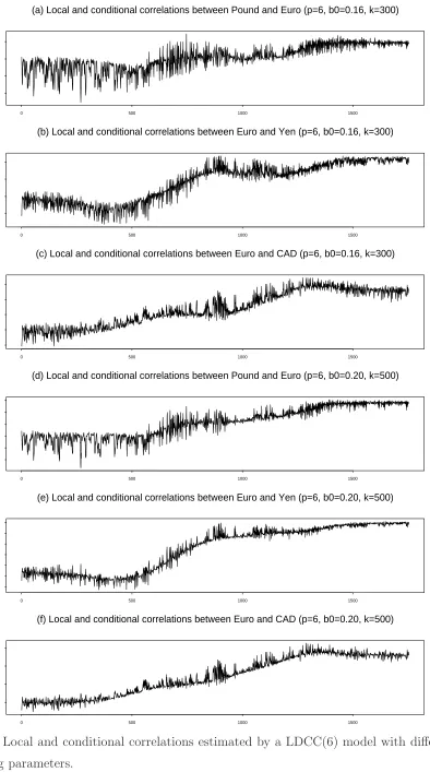
the need of the development of a GARCH-type LDCC model. To show the effect of the
smoothing parameters some further estimation results are given in Figure 5. These are correlations between the Euro and the other currencies estimated using a LDCC(6) model
with smoothing parameters b0 = 0.16 and k = 300 (Figures 5(a) to (c)) and with b0 = 0.20
and k = 500 (Figures 5(d) to (f)), corresponding to those given in Figures 4(a), (d) and (e)
respectively. Comparing the estimates obtained using different smoothing parameters we can
see that they look quite similar to each other. In particular they show the same conditional
patterns. The variations of these estimates depend on the used smoothing parameters.
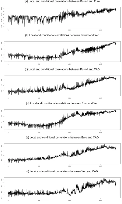
The causal smoother is also applied to these data. Figure 6 shows the estimation results
of a causal LDCC(6) with the same smoothing parameters as for Figure 4. Note that causal
and non-causal estimates are the same for t ≤ k0+p. Comparing Figures 4 and 6 we can
find that, for large t, there are clear differences between the local and conditional patterns
obtained using causal and non-causal methods. The conditional changes are more clear by the causal estimates. We can also see that there is a phase-difference between the periods
estimated by these two approaches where the local correlations increase quickly. The local
changes discovered by the causal estimates seem to be more practically relevant. The
phase-difference in the non-causal estimates is caused by future observations. It is worthwhile to carry out further study on the causal smoother.
The proposed model is also applied to other financial data. In particular, applications to
some weekly UK equity index returns from 1 Jan 1965 to Nov 1999 (Brooks and Henry, 2002)
show that the local and conditional changes in the variances and the conditional changes in
the correlations are more clear in those data. But the local changes in the correlations are not so clear.
6
Final remarks
In this paper simultaneous modelling of local and conditional changes in the variances and correlations of financial returns is discussed. A semiparametric approach is introduced to
model all of these components. In particular the local and conditional correlations are jointly
the theoretical and practical performance of the proposal. So far as we know, this is the first
effort to define and to estimate local and conditional correlations jointly. There are still many open questions in this context, e.g. the development of a suitable bandwidth selection rule,
the development of significance test as well as the the model selection. Finally, the extension
of the current model to a GARCH-type approach by including some latent variables is also of great interest.
Acknowledgments:
The data used in this paper are downloaded from the data releases of the US Federal
Reserve Bank under the address ‘http://www.federalreserve.gov/releases/’. We would like
to thank Prof Chris Brooks, City University London, and Prof Olan Henry, University of Melbourne, for kindly providing us the weekly UK equity index data, to which the model is
also applied. We are very grateful to Prof Winfried Pohlmeier, University of Konstanz, and
Appendix:
Auxiliary results and proofs of theorems
Let ˆξlmt = ˆǫltˆǫmt, l, m = 1, ..., d, denote estimates of ξlmt, where ξlmt are as defined in
Section 4. Let ˜qlm(·) denote the same estimator as ˆqlm(·), but obtained with ˆξlmt being
replaced by ξlmt. To simplify the notations let bµ and bV denote some generic bandwidths
for estimating the mean and variance functions which are of suitable orders depending on
the cases under consideration.
The effect of the errors in ˆµi on ˆσ2i is discussed in Feng and Yu (2005). For the LDCC
model this effect is of the same orders of magnitude. Discussion on the effect of the errors
in ˆσ2
i on ˆθi may be found in Feng (2004). Their results will be adapted to the current case.
We now introduce the following variant of Assumption A1 iii).
A1 iii)′. b
µ and bV satisfy O(n−1/3)< bµ< O(n−1/6) and O(n−1/3)< bV =o(1).
Here ‘<’ or ‘>’ are applied to the orders. Condition A3′ is sufficient but not necessary.
Lemma A.1. Consider 0 < τ < 1. Under the conditions A1 i) and ii), and A1 iii)′ the
error in µˆ(τ) does not affect the asymptotic properties of Vˆ(τ).
This means that ˆV(τ) obtained from the residuals ˆr∗
t has the same asymptotic properties as
that obtained from the unobservable r∗
t.
A sketched proof of Lemma A.1. Results for τ = 1 are discussed in detail in the proof
of Theorem 3 of Feng and Yu (2005). In our case the corresponding results are
1. The additional bias in ˆσ2
i(τ) caused by the error in ˆµi(τ) is of the orderO[b4µ+ (nbµ)−1].
2. The additional variance in ˆσi2(τ) caused by the error in ˆµi(τ) is negligible, if bµ >
O(n−1/2).
For more details we refer the reader to the corresponding proofs given there. Note that there
are some differences between the above results and those given there, because now 0< τ <1
is considered. The bias of ˆσ2
i(·) under the assumption that µi(·) were known is of the order
O(b2
V). Under A1 iii)′ we have O[b4µ+ (nbµ)−1] =o(b2V). Hence, the asymptotic bias of ˆσi2(·)
will not be affected by the error in ˆµi(·). Furthermore, the asymptotic variance of ˆσi2(·) will
also not be affected by the error in ˆµi(·), because bµ> O(n−1/2). ⋄
If ˆµi is estimated data-drivenly as assumed in A1 iii), we have bµi = O(n−1/5). Now A1
iii)′ is fulfilled and the error in ˆµ
i on ˆσi2 is asymptotically negligible. The effect of the error
in ˆσ2
Lemma A.2. Under the same conditions of Lemma A.1 θˆi is root-n consistent and
asymp-totically normal as in the parametric case except for a bias term of the orderO[b2
V +(nbV)−1].
The following lemma quantifies the difference between ˜qlm(·) and ˆqlm(·) caused by the error
in ˆσ2
i(·) and that in ˆθi. Note that the latter is resulted by the former.
Lemma A.3. Under the assumptions of Theorem 1 we have
i) E[ˆqlm(τ;y)−ρlm(τ;y)] =E(˜qlm(τ;y)−ρlm(τ;y)) +O[b2V + (nbV)−1],
ii) var[ˆqlm(τ;y)] = var(˜qlm(τ;y))[1 +o(1)] +O[(nbV)−1] and
iii) cov[ˆqlm(τ;y),qˆrs(τ;y)] =cov[˜qlm(τ;y),q˜rs(τ;y)][1 +o(1)] +O[(nbV)−1].
The additional errors caused by the error in σˆ2
i(·) and that inθˆi are asymptotically negligible.
Proof of Lemma A.3. Observe that
ˆ
ξlmi = ˆǫliˆǫmi =.
σl(τi)σm(τi)√hli√hmi
ˆ
σl(τi)ˆσm(τi) p ˆ hli p ˆ hmi
ξlmi.
We have
ˆ
ξlmi−ξlmi =.
σl(τi)σm(τi)√hli√hmi −σˆl(τi)ˆσm(τi) p ˆ hli p ˆ hmi ˆ
σl(τi)ˆσm(τi) p ˆ hli p ˆ hmi ξlmi
= Op
σl(τi)σm(τi) p
hli p
hmi−σˆl(τi)ˆσm(τi) q ˆ hli q ˆ hmi ξlmi =
O(b2V) +Op(nbV)−1
ξlmi, (A.1)
where the first step is because of ˆσl(τi)ˆσm(τi)
p
ˆ hli
p
ˆ
hmi = Op(1) and the last equation is
obtained by means of Taylor expansion.
Althoughξlmi are iid random variables, ˆξlmi correlate to each other. From (A.1) we have
ˆ
ξlmi =
1 +O(b2V) +Op(nbV)−1
ξlmi.
Straightforward analysis shows that, for i6=j,
cor [ˆξlmi,ξˆlmj] =O[(nbV)−1].
i) The difference in the biases of ˆqlm(·) and ˜qlm(·) caused by that between ˆξlmi andξlmi is of
the same order of magnitude asE[ˆξlmi−ξlmi], provided thatE[ξlmi|y=yi] =ρlm(τi;yi)6= 0
for some i such that P
iwi = O(1), where wi are the weights used in ˆqlm(·). Conditioning
E[ˆξlmi−ξlmi] = E
O(b2V) +Op(nbV)−1
ξlmi
=
O(b2V) +Op(nbV)−1
ρlm(τi;yi). (A.2)
ii) Observe that Pni=1P
j6=iwiwj
.
= 1. We have
var [ˆqlm(τ;y)] =
n X i=1 n X j=1
wiwjcov [ˆξlmi,ξˆlmi]
=
n X
i=1
w2ivar [ˆξlmi] +
n X
i=1
X
j6=i
wiwjcov [ˆξlmi,ξˆlmj]
= var [˜qlm(τ;y)][1 +o(1)] +O[(nbV)−1]. (A.3)
iii) From the calculation of cov [˜qlm(·),q˜rs(·)] given later we can see that the proof of the
result in this part is similar to that in ii). Lemma A.3 is proved. ✸
Remark A.1. If our aim is to test the hypothesis H0 : Rt ≡ Id, then the b2V term in the
additional bias of qˆlm(·) caused by the errors in σˆ2i will vanish.
Proof of Lemma 1. Note that b → 0 as n → ∞. Under the assumptions of Lemma
1 there exists a p-ball around y with radius b for large n and the density on this ball is
approximately 0 < f(y)< ∞. Following the k-NN method the bandwidth b is selected so
that the probability for y within this p-ball is approximately k/k0. Note that k0 = 2. nb0.
Under A7 iii) we have k =Cknbp0+1. This leads to
πp/2bp
Γ(p/2 + 1)f(y)
.
= k
k0
.
= Cknb
p+1 0
2nb0
(A.4)
and
b=. C0b0 with C0 =
Ck
2
Γ(p/2 + 1)
πp/2f(y)
1/p
as given in (12). Lemma 1 is proved. ✸
Lemma A.4. Under the assumptions of Theorem 1 the design density f(y) of y satisfies the assumptions of Lemma 1.
Proof of Lemma A.4. For simplicity let y = yt be an observation point. Assume first
that ǫt are observable. Define Sjt2 = 1I′Rt1I, j = 1, ..., p, where 1I is a vector of ones as
defined before. S2
jt is the variance of the normal random variable
p P j=1
construction of yjt we have yjt = Sjt2Zjt2, where Zjt ∼ N(0,1). Under the assumptions of
Theorem 1 Zjt, j = 1, ..., p, are independent of each other. Therefore yt is a vector of
independent non-standardized χ2
1 random variables with the joint density given by
f(yt) =
√
2Γ(1/2)−p
p Y
j=1
yjt−1/2exp{−yjtSjt−2/2}S
−3
jt . (A.5)
If yt is an interior point, we have 0< f(y)<∞ in a neighbourhood of yt. Furthermore, it
is easy to see that the above approximation holds, if yt are calculated from some consistent
estimates ˆǫt of ǫt. The consistency of ˆǫt is ensured by the conditions of Theorem 1. ✸
Remark A.2. The regressors yjt are squared values of some normal random variables.
There is no boundary effect at a point with yj = 0 for some j. This can be seen from
the form of f(y) given in (A.5). If yj = 0 for some j, we only have observations with
yjt≥yj. But the marginal density for yj tends to infinite in a power rate yjt−1/2 for yjt near
the origin. Choosing bj =O(b20), the resulting bias will be till of the order O(b20).
Proof of Theorem 1. Define ηlmt=ξlmt−ρlm(τt;yt). Then we have
E[ηlmt|yt] = 0 and var [ηlmt|yt] =γlm2 .
Under the assumptions ηlmt and ηlms are conditionally independent for t 6= s. The fact
that ρlm(·) can be estimated fromξlmt using kernel method is based on the following special
conditional nonparametric regression model
ξlmt|yt=ρlm(τt;yt) +ηlmt. (A.6)
Consider first the case with l 6= m. Model (A.6) ensures that ˆqlm(·) has the same
asymp-totic properties as in multivariate kernel regression. Let U =R
(v;u)(v;u)′K
0(τ)K(u)dvdu.
Under A6 we have U =diag(µ2(K0), µ2(K), ..., µ2(K)). Let H =diag(b0, b, ..., b) denote the
bandwidth matrix. We have HH′U = µ
2(K)T, where T is as defined in Theorem 1. Let
h(τ;y) denote the joint density of τ and y. Note that h′
τ(τ;y) ≡ 0 and h(τ;y) ≡ f(y),
because τt are equidistant. Following Lemma A.3 and well known results in multivariate
kernel regression we have:
Bias[ˆqlm(τ;y)] =. Bias[˜qlm(τ;y)]
. = tr
1
2Hlm(τ;y)HH
′
U + ▽h(τ;y)▽
′
lm(τ;y)HH′U
h(τ;y)
.
= 1
2µ2(K)b
2 0tr
Hlm(τ;y)T + 2C02▽
f(y)▽′lm(y)
f(y)
which is Clmµ2(K)b20 as defined in Theorem 1, where the second term in the brackets is not
shared by the local linear approach (see Ruppert and Wand, 1994).
Forl =m, we have ρll(·)≡1. Now ˜qll(·) is unbiased and we have
E[ˆqll(τ;y)−ρll(τ;y)] = O[b2V + (nbV)−1]
= o(b20), (A.8)
which is caused by the error in the estimated variances.
For any l and m the variance of ˆqlm(·) is of the same order. In the current case the
asymptotic variance of ˆqlm(·) is the same as for a local linear estimator. By adapting the
result in (2.4) of Ruppert and Wand (1994) we have
var [ˆqlm(τ;y)] = var [˜. qlm(τ;y)]
.
= 1
nb0bp
R(K0)R(K)
γ2
lm
h(τ;y), (A.9)
where h(τ;y)≡f(y). Observe that
b0bp = C0pbp0+1
= Ck
2
Γ(p/2 + 1)
πp/2f(y)
= kn−1C−1
V R(K0)R(K)f−1(y),
where CV is as defined in Theorem 1. Insert this into (A.9) we have
var [ˆqlm(τ;y)] =. CVk−1γlm2 . (A.10)
Now consider the covariance between ˆqlm(·) and ˆqrs(·) for any {l, m} 6={r, s}. Note that
these two estimators are obtained using the same kernel weights. This results in a close
relationship between cov [ˆqlm(·),qˆrs(·)] and var [ˆqlm(·)] (or var [ˆqrs(·)]). Observe that ξlmi is
independent of ˆξlmj for i6=j. Following Lemma A.3 we have,
cov [ˆqlm(τ;y),qˆrs(τ;y)] = cov [˜. qlm(τ;y),q˜rs(τ;y)]
. =
n X
i=1
n X
j=1
wiwjcov [ξlmi, ξrsj]
. =
n X
i=1
w2icov [ξlmi, ξrsj]
=
n X
i=1
w2iγlm,rs (A.11)
= var [˜qlm(τ;y)]γlm,rs/γlm2
.
Proof of (13). Note thatk =Cknbp0+1. The dominating part of the MSE of ˆqlm(·) is
MSE=. C−1
k CVγ
2
lm nb p+1 0
−1
+Clm2 µ22(K)b40
and
MSE′b0
.
=−(p+ 1)Ck−1CVγlm2 nbp0+2
−1
+ 4Clm2 µ22(K)b30.
Set MSE′
b0 = 0 we obtain
bopt0 =
(p+ 1)CVγlm2
4C2
lmµ22(K)Ck p+51
n−p+51 ,
as given in (13). ✸
The results in Theorem 2 are obtained based on the same results on ˆqlm(·) and ˆqrs(·) given
in the following lemma, where it is assumed that l 6=m,r 6=s and {l, m} 6={r, s}.
Lemma A.5. Under the same conditions of Theorem 2 we have
√
k qˆlm(τ;y)−ρlm(τ;y)
ˆ
qrs(τ;y)−ρrs(τ;y) ! D −→N ( Cµ Clm Crs !
, CV
γ2
lm γlm,rs
γlm,rs γrs2 . !)
, (A.12)
where the constants are the same as defined in Theorem 2.
Proof of Lemma A.5. Following Theorem 1, the squared asymptotic bias and the
asymptotic variance of √kqˆlm(·) are both constants, if b0 = Cbn−
1
p+5 is used. Following
Theorem iii) and iv), it is easy to see that the variances of √kqˆlm(·) and
√
kqˆrs(·), and the
covariance between them are those given in Theorem 2. Note that k =Cknbp0+1. Following
Theorem 1 i) we have
Bias[√kqˆlm(τ;y)] =. Clmµ2(K)Ck1/2C
(p+1)/2
b Cb2
= CµClm,
where Cµ=µ2(K)Ck1/2Cb(p+5)/2 as defined in Theorem 2. Similarly, we have
Bias[√kqˆrs(τ;y)] =. CµCrs.
Following Lemma A.3 we have
√
k{qˆlm(τ;y)−ρlm(τ;y)}=
√
k{q˜lm(τ;y)−ρlm(τ;y)}[1 +op(1)],
√
k{qˆrs(τ;y)−ρrs(τ;y)}=
√
We will prove the asymptotic normality with ˆqlm(·) and ˆqrs(·) being replaced by ˜qlm(·) and
˜
qrs(·) respectively. Note thatηlmtare normally distributed, andηlmiandηlmj are independent
fori6=j. This together with the condition on the bandwidth ensures that√k{q˜lm(·)−ρlm(·)}
is asymptotically normal. Analogously, √k{q˜rs(·)−ρrs(·)}is also asymptotically normal.
Using the Cram´er-Wold device, the joint asymptotic normality of√k{q˜lm(·)−ρlm(·)} and
√
k{q˜rs(·)−ρrs(·)} is proved, if we can show that, for any α1, α2 ∈ ℜ,
√
k{α1[˜qlm(τ;y)−ρlm(τ;y)] +α2[˜qrs(τ;y)−ρrs(τ;y)]}
D
−→N(µ(α1, α2), V(α1, α2)),
where µ(α1, α2) =Cµ(α1Clm+α2Crs) and V(α1, α2) =CV(α21γlm2 +α22γrs2 + 2α1α2γlm,rs). In
the following we will explained briefly that this holds. Let
Z = α1q˜lm(τ;y) +α2q˜rs(τ;y)
= α1
n X
i=1
wiξlmi+α2
n X
i=1
wiξrsi
=
n X
i=1
wi[α1ξlmi+α2ξrsi]. (A.13)
We see that √kZ is asymptotically normal with the given bias and variance. This finishes
the proof of Lemma A.5. ✸
Proof of Theorem 2. Straightforward calculations using Taylor lead to
ˆ
rlm(τ;y)−qˆlm(τ;y) =
ˆ
qlm(τ;y)
√ ˆ
qllqˆmm −
ˆ
qlm(τ;y)
= T1+T2, (A.14)
where T1 = O[b2V + (nbV)−1/2] = o(k−1/2) is the bias term caused by those in ˆqll and ˆqmm,
and T2 = ˆqlm(·)Op(k−1/2), where the Op(k−1/2) term is a random variable with zero mean
caused by the stochastic part of ˆqll and ˆqmm. It is clear that var (T2) =o(k−1). Using similar
idea as in the proof of Lemma A.3, it can be shown that E(T2) = O(k−1). In summary we
have
√
k{rˆlm(τ;y)−ρlm(τ;y)}=
√
k{ˆrlm(τ;y)−ρlm(τ;y)}[1 +o(1)].
This holds of course for ˆrrs(·), too. Analogously, it can be shown that the above
approxi-mation also holds for the difference between α1ˆrlm(·) +α2rˆrs(·) andα1qˆlm(·) +α2qˆrs(·). The
References
Bauwens, L., S. Laurent and J. Rombouts, 2005, Multivariate GARCH models: A survey. CORE discussion paper, 2003/31 (revised 2005).
Beran, J. and Y. Feng, 2002, SEMIFAR models - A semiparametric framework for
mod-elling trends, long-range dependence and nonstationarity. Computational Statistics & Data Analysis, 27, 393-419.
Bollerslev, T, 1986, Generalized Autoregressive Conditional Heteroscedasticity. Journal of
Econometrics, 31, 307-327.
Bollerslev, T., 1990, Modelling the coherence in short-run nominal exchange rates: A
mul-tivariate generalized ARCH model. Review of Economics and Statistics, 72, 498-505.
Bollerslev, T., R. Chou and K. Kroner, 1992, ARCH modeling in finance: A review of the theory and empirical evidence. Journal of Econometrics, 52, 5-59.
Bollerslev, T., R.F. Engle and J.M. Wooldridge, 1988, A Capital Asset Pricing Model with
Time-Varying Covariances. Journal of Political Economy, 96, 116-131.
Brooks, C. and O. Henry, 2002, The impact of news on measures of undiversifiable risk:
Evidence from the UK stock markets. Oxford Bulletin of Econonics and Statistics, 64,
487-507.
B¨uhlmann, P. and A.J. McNeil, 2002, An algorithm for nonparametric GARCH modelling.
Computational Statistics & Data Analysis, 40, 665-683.
Cappiello, L., R.F. Engle and K. Sheppard, 2003, Evidence of Asymmetric Effects in the
Dynamics of International Equity and Bond Return Covariance. Preprint, European Central
Bank.
Dahlhaus, R., 1997, Fitting time series models to nonstationary processes. Annals of Statis-tics, 25, 1-37.
Engle, R.F., 1982, Autoregressive Conditional Heteroscedasticity with Estimates of the
Vari-ance of UK Inflation. Econometrica, 50, 987-1008.
Engle, R.F., 2001, Financial econometrics - A new discipline with new methods. Journal of
Econometrics, 100, 53-56.
Engle, R.F., 2002, Dynamic conditional correlation: A simple class of multivariate
general-ized autoregressive conditional heteroskedasticity models. Journal of Business & Economic
Engle, R.F. and K.F. Kroner, 1995, Multivariate simultaneous GARCH. Econometric
The-ory, 11, 122-150.
Engle, R.F. and K. Sheppard, 2001, Theoretical and empirical properties of dynamic
condi-tional correlation multivariate GARCH. Preprint, Nacondi-tional Bureau of Economic Research.
Fan, J. Q. and Yao, 1998, Efficient estimation of conditional variance functions in stochastic
regression. Biometrika, 85, 645-60.
Feng, Y., 2004, Simultaneously modelling conditional heteroskedasticity and scale change.
Econometric Theory, 20, 563-596.
Feng, Y. and S. Heiler, 1998, Locally weighted autoregression, in: R. Galata and H. K¨uchenhoff
(Eds.) Econometrics in theory and practice, Physica-Verlag, Heidelberg, pp. 101-117.
Feng, Y. and K. Yu, 2005, A Slowly Changing Vector Random Walk Model. Preprint,
Heriot-Watt University and Brunel University.
H¨ardle, W., A.B. Tsybakov and L. Yang, 1998, Nonparametric vector autoregression.
Jour-nal of Statistical Planning and Inference, 68, 221-245.
Hafner, C.M., D. van Dijk and P.H. Franses, 2005, Semi-parametric modelling of correlation dynamics. Research Report, Erasmus University Rotterdam.
Hafner, C.M. and P.H. Franses, 2003, A generalized dynamic conditional correlation model
for many asset returns. Research Report, Erasmus University Rotterdam.
Herzel, S. C. Starica and R. Tutungu, 2006, A non-stationary paradigm for the dynamics of multivariate model for financial returns. Preprints, University of Perugia.
Ling, S. and M. McAleer, 2002, Necessary and sufficient moment conditions for the GARCH(r,s)
and asymmetric power GARCH(r,s) models. Econometric Theory, 18, 722-729.
Pelletier, D., 2006, Regime Switching for Dynamic Correlations. Journal of Econometrics,
131, 445-473.
Ruppert, D. and M.P. Wand, 1994, Multivariate locally weighted least squares regression.
Annals of Statistics, 22, 1346-1370.
Silvennoinen, A. and T. Ter¨asvirta, 2005, Multivariate Autoregressive Conditional Het-eroskedasticity with Smooth Transitions in Conditional Correlations. Preprint, Stockholm
School of Economics.
0 500 1000 1500
-0.02
-0.01
0.0
0.01
0.02
(a) Log-returns of the exchange rates between Pound and USD
0 500 1000 1500
-0.02
-0.01
0.0
0.01
0.02
(b) Log-returns of the exchange rates between Euro and USD
0 500 1000 1500
-0.03
-0.01
0.0
0.01
0.02
0.03
(c) Log-returns of the exchange rates between Yen and USD
0 500 1000 1500
-0.01
0.0
0.01
[image:25.595.88.504.106.613.2](d) Log-returns of the exchange rates between CAD and USD
0 500 1000 1500
0.004
0.005
0.006
0.007
0.008
(a) Estimated total standard deviations for Pound returns
0 500 1000 1500
0.006
0.008
0.010
(b) Estimated total standard deviations for Euro returns
0 500 1000 1500
0.006
0.007
0.008
0.009
(c) Estimated local standard deviations for Yen returns
0 500 1000 1500
0.003
0.004
0.005
0.006
[image:26.595.106.503.103.622.2](d) Estimated total standard deviations for CAD returns
Figure 2: Estimated total standard deviations ˆσi(τt)
p
ˆ
0 500 1000 1500
0.5
0.6
0.7
0.8
(a) Local and conditional correlations between Pound and Euro
0 500 1000 1500
0.0
0.2
0.4
0.6
(b) Local and conditional correlations between Pound and Yen
0 500 1000 1500
0.0
0.2
0.4
(c) Local and conditional correlations between Pound and CAD
0 500 1000 1500
0.0
0.2
0.4
0.6
(d) Local and conditional correlations between Euro and Yen
0 500 1000 1500
0.0
0.2
0.4
0.6
(e) Local and conditional correlations between Euro and CAD
0 500 1000 1500
0.0
0.1
0.2
0.3
0.4
0.5
[image:27.595.107.507.59.718.2](f) Local and conditional correlations between Yen and CAD
Figure 3: Local and conditional correlations estimated by a LDCC(4) model with b0 = 0.18
0 500 1000 1500
0.5
0.6
0.7
0.8
(a) Local and conditional correlations between Pound and Euro
0 500 1000 1500
0.0
0.2
0.4
0.6
(b) Local and conditional correlations between Pound and Yen
0 500 1000 1500
0.0
0.2
0.4
(c) Local and conditional correlations between Pound and CAD
0 500 1000 1500
0.0
0.2
0.4
0.6
(d) Local and conditional correlations between Euro and Yen
0 500 1000 1500
0.0
0.2
0.4
0.6
(e) Local and conditional correlations between Euro and CAD
0 500 1000 1500
0.0
0.1
0.2
0.3
0.4
0.5
[image:28.595.103.508.61.719.2](f) Local and conditional correlations between Yen and CAD
Figure 4: Local and conditional correlations estimated by a LDCC(6) model with b0 = 0.18
0 500 1000 1500
0.5
0.6
0.7
0.8
(a) Local and conditional correlations between Pound and Euro (p=6, b0=0.16, k=300)
0 500 1000 1500
0.0
0.2
0.4
0.6
(b) Local and conditional correlations between Euro and Yen (p=6, b0=0.16, k=300)
0 500 1000 1500
-0.2
0.0
0.2
0.4
0.6
(c) Local and conditional correlations between Euro and CAD (p=6, b0=0.16, k=300)
0 500 1000 1500
0.55
0.65
0.75
(d) Local and conditional correlations between Pound and Euro (p=6, b0=0.20, k=500)
0 500 1000 1500
0.0
0.2
0.4
0.6
(e) Local and conditional correlations between Euro and Yen (p=6, b0=0.20, k=500)
0 500 1000 1500
0.0
0.2
0.4
0.6
[image:29.595.113.507.44.751.2](f) Local and conditional correlations between Euro and CAD (p=6, b0=0.20, k=500)
Figure 5: Local and conditional correlations estimated by a LDCC(6) model with different
0 500 1000 1500
0.50
0.60
0.70
0.80
(a) Local and conditional correlations between Pound and Euro
0 500 1000 1500
0.0
0.2
0.4
0.6
(b) Local and conditional correlations between Pound and Yen
0 500 1000 1500
0.0
0.2
0.4
(c) Local and conditional correlations between Pound and CAD
0 500 1000 1500
0.0
0.2
0.4
0.6
(d) Local and conditional correlations between Euro and Yen
0 500 1000 1500
0.0
0.2
0.4
0.6
(e) Local and conditional correlations between Euro and CAD
0 500 1000 1500
-0.1
0.1
0.3
0.5
[image:30.595.106.507.49.718.2](f) Local and conditional correlations between Yen and CAD
Figure 6: Local and conditional correlations estimated by a LDCC(6) model using causal