http://dx.doi.org/10.4236/ajcm.2014.43012
Nonlinear Interaction of
N
Conservative
Waves in Two Dimensions
Victor A. Miroshnikov
Department of Mathematics, College of Mount Saint Vincent, New York, USA Email: [email protected]
Received 20 February 2014; revised 20 March 2014; accepted 27 March 2014 Copyright © 2014 by author and Scientific Research Publishing Inc.
This work is licensed under the Creative Commons Attribution International License (CC BY). http://creativecommons.org/licenses/by/4.0/
Abstract
Kinematic Fourier (KF) structures, exponential kinematic Fourier (KEF) structures, dynamic ex-ponential (DEF) Fourier structures, and KEF-DEF structures with constant and space-dependent structural coefficients are developed in the current paper to treat kinematic and dynamic prob-lems for nonlinear interaction of N conservative waves in the two-dimensional theory of the New-tonian flows with harmonic velocity. The computational method of solving partial differential eq-uations (PDEs) by decomposition in invariant structures, which continues the analytical methods of undetermined coefficients and separation of variables, is extended by using an experimental and theoretical computation in Maple™. For internal waves vanishing at infinity, the Dirichlet problem is formulated for kinematic and dynamics systems of the vorticity, continuity, Helmholtz, Lamb-Helmholtz, and Bernoulli equations in the upper and lower domains. Exact solutions for upper and lower cumulative flows are discovered by the experimental computing, proved by the theoretical computing, and verified by the system of Navier-Stokes PDEs. The KEF and KEF-DEF structures of the cumulative flows are visualized by instantaneous surface plots with isocurves. Modeling of a deterministic wave chaos by aperiodic flows in the KEF, DEF, and KEF-DEF struc-tures with 5N parameters is considered.
Keywords
Structures, Waves, Computation, Experiment, Theory
1. Introduction
(
)
1t
p
t ρ ν
∂ + ⋅∇ = − ∇ + ∆ +
∂
v
v v v g, ∇ ⋅ =v 0, (1-2) where v=
(
u, 0,w)
is a vector field of the flow velocity, g=(
0, 0,−gz)
is a vector field of the gravitationalacceleration, pt is a scalar field of the total pressure, ∇ = ∂ ∂
(
x, 0,∂ ∂z)
and2 2 2 2
x z
∆ = ∂ ∂ + ∂ ∂ are the gradient and the Laplacian in the 2d Cartesian coordinate system x=
(
x, 0,z)
of the three-dimensional (3d) space with unit vectors(
i j k, ,)
, respectively, and t is time.By a flow vorticity ω=
(
0, , 0υ)
of the velocity field,
∇× =v
ω
(3) Equation (1) may be written into the Lamb-Pozrikidis form [1] [2]1
, 2
t
p
t ρ ν
∂
+ ∇ ⋅ + − ⋅ + × + ∇ × =
∂
v
v v g x ω v ω 0 (4)
which sets a dynamic balance of inertial, potential, vortical, and viscous forces, respectively. Using a dynamic pressure per unit mass [3]
0
,
t d
p p
p ρ −
= − ⋅g x (5) where p0 is a reference pressure, a kinetic energy per unit mass ke= ⋅v v 2 , the 2d Helmholtz
decomposi-tion [4] of the velocity field
φ
= ∇ + ∇×
v ψ (6) and the vortex force
,
d × = ∇ + ∇×v a
ω (7)
Equation (4) is reduced to the Lamb-Helmholtz PDE 0
e e
b
∇ + ∇ ×h = (8) for a scalar Bernoulli potential
e d e
b p k d
t
φ
∂
= + + +
∂ (9)
and a vector Helmholtz potential
,
e
t ν
∂
= + +
∂
h ψ ω a (10) where φ and d are scalar potentials, ψ =
(
0, , 0η)
and a=(
0, , 0b)
are vector potentials, η and b are pseudovector potentials of v and ω×v, respectively. The Lamb-Helmholtz PDE (8) means a dynamic bal-ance between potential and vortical forces of the Navier-Stokes PDE (1), which are separated completely.A linear part of the kinematic problem for free-surface waves of the theory of the ideal fluid with ν =0 im-plies the exponential Fourier eigenfunctions [5], which are obtained by the classical method of separation of va-riables of the 2d Laplace Equation in [4] and [1]. This analytical method was recently developed into the com-putational method of solving PDEs by decomposition into invariant structures. In [3], the Boussinesq-Rayleigh- Taylor structures were developed for topological flows away from boundaries. The trigonometric Taylor struc-tures and the trigonometric-hyperbolic strucstruc-tures [6] were used to describe spatiotemporal cascades of exposed and hidden perturbations of the Couette flow, respectively. In [7], the theory of the invariant trigonometric, hyperbolic, and elliptic structures was constructed and applied for modeling dual perturbations of the Poi-seuille-Hagen flow.
lower domains and treated in the KF and KEF structures. To compute and explore Jacobian determinants (JDs) of the velocity field, the DEF structure is also constructed in this section. In section 3, the dynamic problems for the Bernoulli potential and the total pressure are formulated and computed in the KF, KEF, and KEF-DEF structures. The Navier-Stokes system of PDEs is employed for verification of experimental and theoretical solu-tions for cumulative upper and lower flows in this section, as well. Visualization and discussion of the devel-oped structures and fluid-dynamic variables is given in section 4, which is followed by a summary of main re-sults in Section 5.
2. Kinematic Problems for Conservative Flows
The following solutions and admissible boundary conditions for the kinematic problems of section 2 in the KF and DEF structures were primarily computed experimentally in Maple™ by programming with lists of equations and expressions in the virtual environment of a global variable Eqs with 29 procedures of 670 code lines.
2.1. Formulation of Theoretical Kinematic Problems for Velocity Components
Theoretical kinematic problems for harmonic velocity components u=u x z t
(
, ,)
and w=w x z t(
, ,)
of a cu-mulative flow v=ui+wk of a Newtonian fluid are given by vanishing they-component of the vorticity Equa-tion (3) and the continuity EquaEqua-tion (2), respectively,0,
u w
z x
∂ −∂ =
∂ ∂ 0.
u w
x z
∂ +∂ =
∂ ∂ (11-12)
To consider nonlinear interaction of N internal, conservative waves with a harmonic velocity field, the cu-mulative flow is decomposed into a superposition of local flows
(
)
(
)
1 1
, , , , , ,
N N
n n
n n
u u x z t w w x z t
= =
=
∑
=∑
(13)such that the local vorticity and continuity equations are
0, 0,
n n n n
u w u w
z x x z
∂ −∂ = ∂ +∂ =
∂ ∂ ∂ ∂ (14-15)
where n=1, 2,, .N If Equations (14)-(15) for the local flows are fulfilled, then substitution of superpositions (13) into (11)-(12) and changing order of summation and differentiation yield that Equations (11)-(12) for the cumulative flow are also satisfied.
Upper flows are specified by the Dirichlet condition in the KF structure on a lower boundary z=0 of an upper domain x∈ −∞ ∞
(
,)
and z∈[
0,∞)
(seeFigure 1)0
nz n n n n
w = =Fw ca +Gw sa (16)
and a vanishing condition as z→ ∞
0.
n z
w =∞ = (17) Lower flows are identified by the Dirichlet condition on a lower boundary z=0 of a lower domain
(
,)
x∈ −∞ ∞ and z∈ −∞
(
, 0]
(seeFigure 1)0
nz n n n n
w = =Fw ca +Gw sa (18)
and a vanishing condition as z→ −∞
0.
n z
w =−∞ = (19) Thus, an effect of surface waves on the internal waves is described by the Dirichlet conditions (16) and (18). Here, a structural notation
( )
( )
cos , sin ,
n n n n
ca = α sa = α (20)
is used for kinematic structural functions can and san, where Fwn and Gwn are boundary coefficients, n nXn
Figure 1. Configuration of upper and lower domains for internal, conserva-tive waves.
gation coordinate, ρn is a wavenumber, Cxn is a celerity, and Xan is an initial coordinate for all n.
As we will see later, boundary conditions for un are then redundant since boundary parameters of un
0 ,
nz n n n n
u = = −Gw ca +Fw sa
0
n z n n n n
u = =Gw ca −Fw sa (21-22)
for the upper and lower flows, respectively, depend on boundary parameters of wn. Similarly to wn, un
va-nishes as z→ ±∞
0,
n z
u =∞ = un z=−∞ =0, (23-24) for the upper and lower flows, respectively.
Thus, thex-andz-components of the velocity field of the cumulative flows are expanded in the KF structures with constant structural coefficients
(
)
(
)
1 1
0 , 0 ,
N N
n n
n n n n n n n n
z z
u = Gw ca Fw sa w = Fw ca Gw as
= =
=
∑
− + =∑
+ (25)(
)
0(
)
1 1
0 n n n n , n n n n ,
z z
N N
n n
u Gw ca Fw sa w Fw ca Gw sa
= =
= =
∑
− = =∑
+ (26)and the velocity components vanish as z→ ±∞
0, 0,
z z
u =∞= w =∞= (27)
0, 0,
z z
u =−∞ = w =−∞= (28) for the upper and lower cumulative flows, respectively.
2.2. Theoretical Solutions for the Velocity Field
Theoretical solutions of kinematic problems (11)-(28) are constructed in the KF structure p x z t
(
, ,)
of two spatial variables x z, , and time t with a general term pn, which in the structural notation may be written as(
)
(
)
(
( )
( )
)
1 1
, , , , ,
N
n n n n n
N n
n
p x z t p x z t fp z ca gp z sa
= =
where first letters f and g of structural coefficients fpn
( )
z and gpn( )
z refer to the kinematic structuralfunctions ca san, n and a second letter to the expanded variable p. Thus, general terms of the velocity
compo-nents of the local flows in the structural notation become
( )
( )
,n n n n n
u = fu z ca +gu z sa wn= fwn
( )
z can+gwn( )
z san. (30-31) It may be shown that spatial derivatives of pn are( )
( )
(
)
,n
n n n
n n
p
gp z ca fp z sa
x ρ
∂
= −
∂
d d
d .
d
n n n n n
p fp gp
ca sa
z z z
∂
= +
∂ (32-33)
Application of (32)-(33) to (30)-(31), substitution in (14)-(15), and collection of the structural functions re-duce the vorticity and continuity PDEs to the following system of two vorticity and continuity ordinary differen-tial equations (ODEs) in the KF structures:
d d
0,
d d
n n
n n n
n n
n
fu gu
gw ca fw sa
z ρ ρ z
− + =
+
d d
0.
d d
n n
n n n n n n
fw gw
gu ca fu sa
z ρ ρ z
+ + − + =
(34-35)
For Equations (34)-(35) to be satisfied exactly for all variables, parameters, and functions of the local flows:
,
x z, t, αn, ρn, fun, gun, fwn, and gwn, all coefficients of two kinematic structural functions must
vanish. Thus, two ODEs (34)-(35) are reduced to two systems of ODEs for fun, gwn and fwn, gun,
re-spectively:
d
0, d
n
n n
fu
gw
z −ρ =
d
0, d
n n n
gw fu
z
ρ
− + = (36-37) d
0, d
n n n
gu fw
z
ρ + = d 0.
d
n
n n
fw
gu
z +ρ = (38-39)
Since boundary conditions (25)-(26) are expanded in the KF structure exactly, remainders of structural ap-proximations (34)-(35) vanish, and exact solutions of ODEs (36)-(39) produce exact solutions of vorticity and continuity PDEs (14)-(15). If (25)-(26) are replaced with series approximations, then their remainders constitute errors of the series approximations.
Solutions of ODEs for structural coefficients (36)-(39) are constructed in an exponential structure
(
, , ,) (
, , ,)
ec zn ,n n n n n n n n
fu gu fw gw = Fu Gu Fw Gw (40)
where Fu Gu Fw Gwn, n, n, n, and cn are structural coefficients. Substitution of exponential structure (40) in
Equations (36) and (38) reduces these ODEs to algebraic equations (AEs) for structural parameters:
, .
n n n n
n n
n n
Gw Fw
Fu Gu
c c
ρ ρ
= = − (41)
Substitution of (40) and (41) in (37) and (39) reduces these ODEs to AEs for admissible values of the struc-tural coefficient cn with the following solutions for the upper and lower flows, respectively:
, .
n n n n
c = −ρ c =ρ (42) Since the admissible values of cn coincide for Equations (37) and (39), ODEs for structural coefficients
(36)-(39) are compatible both for the upper and lower flows.
Finally, substitutions of (40)-(42) in (30)-(31) and (13) yield the velocity components in the KEF structures for the upper cumulative flow
(
)
(
)
1
, , e n ,
N
z n n n n n
u x z t Gw ca Fw sa −ρ
=
=
∑
− +(
)
(
)
1
, , e n ,
N
z n n n n n
w x z t Fw ca Gw sa −ρ
=
=
∑
+ (43-44)and the lower cumulative flow
(
)
(
)
1
, , e n ,
N
z n n n n n
u x z t Gw ca Fw sa ρ
=
=
∑
−(
)
(
)
1
, , e n ,
N
z n n n n n
w x z t Fw ca Gw sa ρ
=
=
∑
+ (45-46)2.3. The DEF structure and Theoretical Jacobian Determinants of the Velocity Components
Define two KEF structures l x z t
(
, ,)
and h x z t(
, ,)
with general terms ln and hm by using a generalizedEinstein notation for summation, which is extended for exponents,
(
)
(
)
(
)
(
)
1 1
, , e n , , , e m .
N N
z z
n n n n n m m m m m
n m
l x z t l Fl ca Gl sa ρ h x z t h Fh ca Gl sa ρ
= =
=
∑
= + =∑
= + (47) Computation of a general termpn n, =l hn nby summation of diagonal terms yields
(
)
(
(
)
)
2, e n 2.
z
n n n,n n n n n n,
n n Fl Fhn n Gl Ghn n Fl Fhn Gl Gh Casn Fl Gh Fh Gl Sa n
p = + + − + + s ρ (48)
Trigonometric structural functions Casn m, , Cadn m, , Sasn m, , and Sadn m, of the DEF structure are defined
by the following expressions:
(
)
(
)
(
)
,(
)
cos , cos , sin , sin ,
n,m n m n,m n m n,m n m n m n m
Cad = α −α Cas = α +α Sad = α −α Sas = α +α (49)
where capital letters C and S stand for dynamic structural functions cosine and sine, letter a for arguments , ,
n m
α α and letters s and d for sum and difference of arguments αn and αm.
A general term pn m, =l hn m computed by rectangular summation of non-diagonal terms becomes
(
)
(
)
(
(
)
(
)
)
( ),
.
e n m 2
n m n m n m n,m n m n n,m n,m
z n,m
m n m m n
n m m n
Fl Fh Gl Gh Cad Fl Gh Cas Fl Fh Sad
Fl Gh Fh Gl
p Fh Gl Gh Gl
Sas ρ +ρ
= +
+
− − +
+
+ +
(50)
By triangular summation, pn m, is reduced to
( )
(
(
)
(
)
(
)
(
)
)
, e 2
.
n m
n m n m m n n m m n n m m n n m m n
n m n m m n n m m n
z
n,m n,m
m n n,
n
m , m m n n m
Fl Fh Fl Fh Gl Gh Gl Gh Cad
Fl Fh Fl Fh Gl Gh Gl Gh Ca
p
s
Fl Gh Fl Gh Fh Gl Fh Gl Sad
Fl Gh Fl Gh Fh Gl Fh Gl Sas
ρ +ρ
= × + + +
+ + − −
+ − − +
+ + + +
+
(51)
Using general terms (48) and (51), summation formula for the product of the KEF structures is written as the DEF structure
(
) (
) (
)
(
)
(
)
( )2
1 1
, , ,
1 1
1
, , , , , , e
2 1
e 2
n
m n
z n,n n,n n,n n,n n,n n
N N
z n m n,m n m n,m n m n,m n,m n,m
n m n
N
p x z t l x z t h x z t Fdp Fsp Cas Gsp Sas
Fdp Cad Fsp Cas Gdp Sad Gsp Sas
ρ
ρ ρ =
−
+
= = +
= = +
+ + + +
+
∑
∑ ∑
(52)
with the following structural coefficients:
, ,
, ,
, ,
, , ,
, ,
,
n m n,n n n n n n n n n
n
n n n n n n
n m m n n m m n n m m n n m m n
n m n m m n n m m n
m n m
n m m n n m n m m
Fdp Fl Fh Gl Gh Fsp Fl Fh Gl Gh Gsp Fl Gh Fh Gl
Fdp Fl Fh Fl Fh Gl Gh Gl Gh Fsp Fl Fh Fl Fh Gl Gh Gl Gh
Gdp Fl Gh Fl Gh Fh Gl Fh Gl Gsp Fl Gh Fl Gh Fh Gl Fh
= + = − = +
= + + + = + − −
= − + − + = + + + Gln,
(53)
where first two letters Fd, Fs, Gd, and Gs of structural coefficients Fdpn m, , Fspn m, , Gdpn m, , and ,
n m
Gsp stand for dynamic structural functions Cadn, Casn, Sadn, and Sasn, respectively, and a third letter
for variable p.
Computation of local JDs for the velocity components of the upper and lower flow, respectively, yields
(
2 2)
2e2 nz.n n n n
n n n
u w u w
Fw Gw
x z z x
ρ
ρ
∂ ∂ −∂ ∂ = − +
∂ ∂ ∂ ∂ (54)
Thus, velocity components un and wn are independent for non-trivial structural coefficients Fwn and n
Gw since the local JDs vanish when Fw2n+Gw2n =0.
(
)
(
)
(
(
)
)
( )1
,
1 1
2
,
2 2 2
1
2
e .
e
n n
m N N
n m n m n m n m n
n m m n n m N
z
g n n n
n
z n m
Fw Fw Gw Gw Cad
Fw Gw Fw Gw Sa
u w u w
J Fw Gw
x z z x
d
ρ
ρ ρ
ρ
ρ ρ
− = = +
=
+
+
∂ ∂ ∂ ∂
= − = − +
∂ ∂ ∂ ∂
− +
+ −
∑ ∑
∑
(55)
So, Jg is a superposition of a propagation JD with general term Jcn n, proportional to Cadn n, ≡1, an
in-teraction JD with Jcn m, proportional to Cadn m, , and an interaction JD with Jsn m, proportional to Sadn m, ,
which describe interaction between parallel and orthogonal internal waves, respectively.
,
n n
Jc coincides with (54). They describe propagation of internal waves and vanish only for internal waves with Fwn2+Gw2n =0. Jsn m, vanishes for parallel waves with
, .
m m
n m
n n
Fw Gw
A
Fw = Gw = (56)
Global JD (55) then becomes
(
)
1(
)
( )2
2 2 2 2 2
, ,
1 1 1
e n 2 e n m .
N N N
z
p n n n n m n n n m n m
n n m n
z
J Fw Gw ρ ρ A Fw Gw ρ ρ Cad ρ ρ
−
+
= = = +
= −
∑
+ −∑ ∑
+ (57)Thus, the global JD does not vanish for parallel waves with non-vanishing Fwn2+Gwn2.
,
n m
Jc vanishes for orthogonal waves with
, .
m m
n m
n n
Fw Gw
B
Gw = −Fw = (58)
In this case, global JD (55) is reduced to
(
)
1(
)
( )2
2 2 2 2 2
, ,
1 1 1
e n 2 e n m .
N N N
z
o n n n n m n n n m n m
n n m n
z
J Fw Gw ρ ρ B Fw Gw ρ ρ Sad ρ ρ
−
+
= = = +
= −
∑
+ −∑ ∑
+ (59)Thus, the global JD does not vanish also for orthogonal waves with non-vanishing Fw2n+Gw2n. In the gener-al case (55) of slant interngener-al waves, both Jsn m, and Jcn m, are non-vanishing. So, both propagating and
inte-racting waves are independent for structural coefficients with Fwn2+Gwn2 ≠0 for all n.
2.4. Theoretical Solutions for the Pseudovector and Scalar Potentials in the KEF Structures
Theoretical kinematic problems for cumulative pseudo-vector potential η
(
x z t, ,)
and cumulative scalar potential φ(
x z t, ,)
of v are set by the global Helmholtz PDEs (6)0, 0,
u w
z x
η η
∂ + = ∂ − =
∂ ∂ (60)
0, 0,
u w
x z
φ φ
∂ − = ∂ − =
∂ ∂ (61)
since the potential-vortical duality the velocity field admits two presentations: v= ∇φ for ψ =0 and
= ∇×
v ψ for φ=0. The cumulative kinematic potentials are decomposed into a superposition of local kine-matic potentials
(
)
(
)
1 1
, , , , , ,
N N
n n
n n
x z t x z t
η η φ φ
= =
=
∑
=∑
(62)such that the local Helmholtz PDEs are
0, 0,
n n
n n
u w
z x
η η
∂ ∂
+ = − =
∂ ∂ (63)
0, 0,
n n
n n
u w
x z
φ φ
∂ − = ∂ − =
where n=1, 2,, .N The boundary conditions for ηn and ϕn and redundant when the problem is
formu-lated in the KF structures.
Construct general terms of the kinematic potentials of the local flows in the KF structure with space-depen- dent coefficients
( )
( )
,n n n n n fe z ca ge z sa
η = + φn= fpn
( )
z can+gpn( )
z san. (65-66) Application of (32)-(33) to (65)-(66), substitution in (63)-(64), and collection of the structural functions re-duce four Helmholtz PDEs to the following system of two Helmholtz ODEs and two Helmholtz AEs for the up-per flows(
)
(
)
d d
0, 0
e ,
d e d e e
nz nz nz nz
n n
n n n n n n
n n n n n n
fe ge
Gw ca Fw sa ge Fw ca fe Gw sa
z z
ρ ρ ρ ρ ρ ρ
− − − −
− + − + =
+ = −
(67-68)
(
e)
(
e)
0, d e d e 0,d d
nz nz nz n
n n n n
z
n n
n n n n n n n n
fp gp
gp Gw ca fp Fw sa Fw ca Gw sa
z z
ρ ρ ρ ρ
ρ + − ρ + − − − + − − =
− = (69-70)
and the lower flows
(
)
(
)
e e
d d
0, 0,
d e e
d
nz nz nz nz
n n
n n n n n n n
n F n n n n
fe ge
Gw ca w sa ge Fw ca fe Gw sa
z z
ρ ρ ρ ρ ρ ρ
+ + − = − + =
−
(71-72)
(
)
(
)
d d0, e e .
d d
e nz enz n nz n nz 0
n n
n n n n n n n n n n
fp gp
gp Gw ca fp Fw sa Fw ca Gw sa
z z
ρ ρ ρ ρ
ρ − ρ − = − + − =
−
(73-74)
For Equations (67)-(74) to be satisfied exactly for all variables, parameters, and functions of the upper and lower flows: , , ,x z tα ρn, n,fe gen, n,fp gp Fwn, n, n, and Gwn, all coefficients of structural functions can and
n
sa must vanish. Thus, two Helmholtz ODEs and two Helmholtz AEs are reduced to the following four AEs and four ODEs with respect to fen, gen, fpn, and gpn for the upper flows
0, 0, 0, 0,
e nz e nz e nz e nz
n n
nfen Gw ngen Fw nfpn Fwn ngpn Gwn
ρ ρ ρ ρ
ρ + − = ρ − − = ρ + − = ρ + − =
(75)
d d d d
0, 0, 0, 0,
e
d d e d e d e
nz nz nz nz
n n
n n n n
n n
fe ge fp gp
Gw Fw Fw Gw
z z z z
ρ ρ ρ ρ
− − − −
− = + = − = − = (76)
and the lower flows
0, 0,
e n en en 0, en 0,
n
z z
n n n n n n
z
n n n n n
z
fe Gw ρ ge Fw ρ fp Fw ρ gp Gw ρ
ρ + = ρ − = ρ − = ρ − = (77)
d d d d
0, 0, 0, 0.
d e d e d e d e
n n n n
n
z z z z
n n n n n n n
fe ge fp gp
Gw Fw Fw Gw
z z z z
ρ ρ ρ ρ
+ = − = − = − = (78)
Since general terms of remainders of structural approximations (67)-(74) vanish, exact solutions of AEs and ODEs (75)-(78) produce exact solutions of the Helmholtz PDEs (63)-(64).
Solving AEs (75) and (77) with respect to fen, gen, fpn, and gpn gives for the upper flows
e nz, e nz, e nz, e nz,
n n n n
n n n n
n n n n
Gw Fw Fw Gw
fe ρ ge ρ fp ρ gp ρ
ρ ρ ρ ρ
− − − −
= − = = − = − (79)
and the lower flows
e nz, e nz, enz, e nz.
n n n n
n n n n
n n n n
Gw Fw Fw Gw
fe ρ ge ρ fp ρ gp ρ
ρ ρ ρ ρ
= − = = = (80)
Substitution of solutions (79)-(80) in ODEs (76) and (78) reduces them to identities.
Substitution of structural coefficients (79)-(80) in the KF structures (65)-(66) and super positions (62) re-turns the cumulative pseudo vector and scalar potentials in the KEF structures for the upper cumulative flow
(
)
(
)
1 1
, , e n ,
N
z n n n n n n
x z t Gw ca Fw sa ρ
η ρ − = =
∑
− +(
)
(
)
1 1, , e n ,
N
z n n n n n n
x z t Fw ca Gw sa ρ
φ
ρ −
=
and the lower cumulative flow
(
)
(
)
1 1
, , en ,
N
z n n n n n n
x z t Gw ca Fw sa ρ
η
ρ
=
=
∑
− +(
)
(
)
1 1
, , e n .
N
z n n n n n n
x z t Fw ca Gw sa ρ
φ
ρ
=
=
∑
+ (83-84)2.5. Harmonic Relationships for the Velocity Components and the Kinematic Potentials
Comparison of solutions for un and wn with spatial derivatives in x of wn and un shows that they are
directly proportional to each other, respectively, for the upper flows
1 1
, ,
n n
n n
n n
w u
u w
x x
ρ ρ
∂ ∂
= − =
∂ ∂ (85)
and the lower flows
1 1
, .
n n
n n
n n
w u
u w
x x
ρ ρ
∂ ∂
= = −
∂ ∂ (86)
In fluid dynamics, these connections mean that a non-uniform vertical flow generates a horizontal flow and a non-uniform horizontal flow produces a vertical flow.
Similarly, comparison of solutions for ηn and φn with solutions for un and wn shows that they are also
directly proportional, respectively, for the upper flows
, ,
n n
n n
n n
u w
η φ
ρ ρ
= = − (87)
and the lower flows
, .
n n
n n
n n
u w
η φ
ρ ρ
= − = (88)
Finally, comparison of solutions for ηn and φn with spatial derivatives in x of φn and ηn shows that
they are proportional to each other, respectively, for the upper flows
1 1
, ,
n n
n n
n x n x
φ η
η φ
ρ ρ
∂ ∂
= = −
∂ ∂ (89)
and the lower flows
1 1
, .
n n
n n
n x n x
φ η
η φ
ρ ρ
∂ ∂
= − =
∂ ∂ (90)
Connections (85)-(90) between solutions in the KEF structures are available since there are only two inde-pendent combinations of trigonometric structural functions Fw can n+Gw san n and Gw can n−Fw san n.
Computation of ∇ ⋅∇ηn φn by using (81)-(84) both for the upper and lower flows gives
0.
n n n n
x x z z
η φ η φ
∂ ∂ ∂ ∂
+ =
∂ ∂ ∂ ∂ (91)
Thus, local isocurves of ηn and φn remain orthogonal for all times in agreement with the Helmholtz
Equa-tions (63)-(64). Similarly, local isocurves ofunandwnremain orthogonal since both for the upper and lower
flows
0,
n n n n
u w u w
x x z z
∂ ∂ +∂ ∂ =
∂ ∂ ∂ ∂ (92)
in agreement with the local vorticity and continuity Equations (14)-(15).
Computation of ∇ ⋅∇η φ by (52)-53) and (81)-(84) both for the upper and lower cumulative flows gives 0.
x x z z
η φ η φ
∂ ∂ +∂ ∂ =
∂ ∂ ∂ ∂ (93)
upper and lower cumulative flows
0,
u w u w
x x z z
∂ ∂ +∂ ∂ =
∂ ∂ ∂ ∂ (94)
in agreement with the cumulative vorticity and continuity Equations (11)-(12).
It is a straightforward matter to show that for the KEF structure p x z t
(
, ,)
with a general term pn(
)
(
)
1
, , e n ,
N
z n n n n n n
p x z t p Fp ca Gp sa ρ
=
=
∑
= + (95) spatial derivatives of second order in the x- and -z directions are
(
)
2
2
2 e ,
nz
n
n n n n n
p
Fp ca Gp sa
x
ρ
ρ
∂ = − +
∂
2 2
(
)
2 e ,
nz
n
n n n n n
p
Fp ca Gp sa
z
ρ
ρ
∂ = +
∂
(96-97) and the Laplacian of pn vanishes. Thus, the KEF structure is an invariant, harmonic structure both for the
up-per and lower flows.
Application of (96)-(97) to (43)-(46) shows that un and wn are conjugate harmonic functions since
2 2 2 2
2 2 0, 2 2 0
n n n n
u u w w
x z x z
∂ +∂ = ∂ +∂ =
∂ ∂ ∂ ∂ (98)
both for the upper and lower flows, in agreement with vector identity ∆ = −∇×vn ωn+ ∇ ∇ ⋅
(
ωn)
=0. By Equ-ations (13), u and w are also conjugate harmonic functions2 2 2 2
2 2 0, 2 2 0,
u u u u
x z x z
∂ +∂ = ∂ +∂ =
∂ ∂ ∂ ∂ (99)
both for the upper and lower cumulative flows, in agreement with vector identity ∆ = −∇× + ∇ ∇ ⋅v ω
(
ω)
=0. Similarly, applying (96)-(97) to (81)-(84) shows that ηn and φn are conjugate harmonic functions as2 2 2 2
2 2 0, 2 2 0
n n n n
x z x z
η η φ φ
∂ +∂ = ∂ +∂ =
∂ ∂ ∂ ∂ (100)
both for the upper and lower flows, in agreement with ∇ ⋅vn = ∇ ⋅∇ = ∆ =φn φn 0 and
(
)
(
)
0.n n n n n
∇×v = ∇× ∇×ψ = ∇ ∇ ⋅ψ − ∆ψ = −∆ψ = By Equation (62), η and φ are also conjugate har-monic functions
2 2 2 2
2 2 0, 2 2 0
x z x z
η η φ φ
∂ +∂ = ∂ +∂ =
∂ ∂ ∂ ∂ (101)
both for the upper and lower cumulative flows, in agreement with vector identities ∇ ⋅ = ∇ ⋅∇ = ∆ =v φ φ 0 and
(
)
(
)
0.∇× = ∇× ∇×v ψ = ∇ ∇ ⋅ψ − ∆ = −∆ =ψ ψ
The theoretical solutions in the KEF and DEF structures for the kinematic problems of section 2 were com-puted theoretically in Maple™ by programming with symbolic general terms in the virtual environment of a global variable Equation with 26 procedures of 591 code lines. The theoretical solutions for velocity compo-nents (43)-(46), the products of the KEF structures (52)-(53), and the kinematic potentials (81)-(84) of the upper and lower cumulative flows were justified by the correspondent experimental solutions for N=1,3,10.
3. Dynamic Problems for Conservative Flows
The following solutions for the dynamic problems of section 3 in the KF, DEF, and KEF-DEF structures were primarily computed experimentally by programming with lists of equations and expressions in the virtual envi-ronment of the global variable Equations with 19 procedures of 472 code lines.
3.1. Theoretical Solutions for the Helmholtz and Bernoulli Potentials in the KEF Structures
cumu-lative flows are set by the Lamb-Helmholtz PDEs (8) 0, e e b h x z ∂ −∂ =
∂ ∂ e e 0,
b h
z x
∂ +∂ =
∂ ∂ (102-103)
while (10) for the vortical presentation with φ=0 is reduced to . e h t η ∂ =
∂ (104)
Equations (102-104) are complemented by the local Lamb-Helmholtz PDEs 0, n n be he x z ∂ ∂ − =
∂ ∂ n n 0,
be he
z x
∂ ∂
+ =
∂ ∂ (105-106)
where , n n he t η ∂ =
∂ (107)
since the cumulative dynamic potentials are again decomposed into the local dynamic potentials as follows:
(
)
(
)
1 1
, , , , , .
N N
e n e n
n n
h he x z t b be x z t
= =
=
∑
=∑
(108)Boundary conditions are again redundant because the problem is formulated in the KF structures.
Construct a general term of the Bernoulli potential of the local flows in the KF structure with space-dependent coefficients
( )
( )
.n n
n n n
be = fb z ca +gb z sa (109) Computation of the temporal derivative of ηn, application of (32)-(33), substitution in (105)-(106), and collection of the structural functions reduce two Lamb-Helmholtz PDEs to the following system of the Lamb-Helmholtz AE and ODE for the upper flows
(
e)
(
e)
e e 0, d d 0, d d n n n n
n n n n n n n
z z
n n n
z z
n n
n n n
n n n n n
gb Cx Fw ca fb Cx Gw sa
fb gb
Cx Gw ca C Fx w sa
z z ρ ρ ρ ρ ρ ρ ρ ρ − − − − − + = − + = + − (110)
and the lower flows
(
)
(
)
0,d d 0. d d e e e e n n n n z z
n n n
z z
n n n n n n n
n n n n n
n n
n n n
gb Cx Fw ca fb Cx Gw sa
fb gb
Cx Gw ca Cx w sa
z z F
ρ ρ ρ ρ ρ ρ ρ ρ + − = − + = − + (111)
For Equations (110)-(111) to be satisfied exactly for all x z t, , ,α ρn, n,Cxn,fb gb Fwn, n, n, and Gwn all
coef-ficients of structural functions can and san must vanish. Thus, the Lamb-Helmholtz AE and ODE are
re-duced to the following two AEs and two ODEs for space-dependent structural coefficients fbn and gbn for
the upper flows
e 0, e 0,
e 0, e 0
d d
,
d d
n n
n n
n n n n
z z
n n
n n n z n n z n n n
fb Cx Gw gb Cx Fw
fb gb
Cx Gw Cx w
z z F
ρ ρ ρ ρ ρ ρ − − − − + = − = + = =
− (112-113)
and the lower flows
e 0, e 0,
e 0, e 0.
d d
d d
n n
n n
z z
n n n n n
n n n n n
n
z z
n n
n
fb Cx Gw gb Cx Fw
fb gb
Cx Gw Cx w
z z F
Since general terms of remainders of structural approximations (110)-(111) vanish, exact solutions of (112)-(115) produce exact solutions of (105)-(106).
Solving AEs (112) and (114) for structural coefficients fbn and gbn yields for the upper flows
e nz, e nz,
n n n n n n
fb = −Cx Gw −ρ gb =Cx Fw −ρ (116)
and the lower flows
enz, e nz.
n n n n n n
fb =Cx Gw ρ gb = −Cx Fw ρ (117)
Substitution of solutions (116)-(117) in ODEs (113) and (115) reduced them to identities.
Substitution of structural coefficients (116)-(117) in super positions (108) and the KF structure (109) gives the cumulative Helmholtz and Bernoulli potentials in the KEF structures for the upper cumulative flow
(
)
(
)
1
, , e n ,
N
z e n n n n n
n
h x z t Cx Fw ca Gw sa −ρ
=
= −
∑
+(
)
(
)
1
, , e n ,
N
z e n n n n n
n
b x z t Cx Gw ca Fw sa −ρ
=
=
∑
− + (118-119)and the lower cumulative flow
(
)
(
)
1
, , e n ,
N
z e n n n n n
n
h x z t Cx Fw ca Gw sa ρ
=
= −
∑
+(
)
(
)
1
, , en .
N
z e n n n n n
n
b x z t Cx Gw ca Fw sa ρ
=
=
∑
− (120-121)Similar to the kinematic potentials (87)-(88), the dynamic potentials and the velocity components are di-rectly proportional both for the upper and lower flows
, .
n n n n n n
he = −Cx w be =Cx u (122) Like in (89)-(90), the Helmholtz and Bernoulli potentials and derivatives of the Bernoulli and Helmholtz potentials inxare directly proportional to each other both for the upper flows
1 1
, ,
n n
n n
n n
be he
he be
x x
ρ ρ
∂ ∂
= − =
∂ ∂ (123)
and the lower flows
1 1
, .
n n
n n
n n
be he
he be
x x
ρ ρ
∂ ∂
= = −
∂ ∂ (124)
Analogous to (91)-(94), isocurves of he ben, n and global isocurves of h be, e are orthogonal for all times
0,
n n n n
he be he be
x x z z
∂ ∂ +∂ ∂ =
∂ ∂ ∂ ∂ 0.
e e e e
h b h b
x x z z
∂ ∂ +∂ ∂ =
∂ ∂ ∂ ∂ (125-126)
in agreement with the Lamb-Helmholtz Equations (105)-(106) and (102)-(103). For the same reason, he ben, n
and h be, e are local and global conjugate harmonic functions as
2 2
2 2 0,
n n
he he
x z
∂ +∂ =
∂ ∂
2 2
2 2 0,
n n
be be
x z
∂ +∂ =
∂ ∂
2 2
2 2 0,
e e
h h
x z
∂ +∂ =
∂ ∂
2 2
2 2 0.
e e
b b
x z
∂ +∂ =
∂ ∂ (127-128)
3.2. Theoretical Solutions for the Total Pressure in the KEF-DEF Structures
Theoretical dynamic problems in the KEF-DEF structures for the kinetic energy per unit mass ke, the dy-namic pressure per unit mass pd, and the total pressure pt of the cumulative flows are formulated by
de-finition
(
2 2)
1
( , , ) ( , , ) ( , , ) , 2
e
k x z t = u x z t +w x z t (129) the Bernoulli Equation (9) with φ=0
(
, ,)
(
, ,)
(
, ,)
,d e e
p x z t =b x z t −k x z t (130)
and the hydrostatic Equation (5)
(
, ,)
0(
, ,)
,t z d
where p0 is the reference pressure at z=0.
Computation of ke by (52)-(53) and (43)-(46) returns
(
)
(
)
(
(
)
(
)
)
( ) 1 2 2 2 ,1 1 1
,
1
, , e
2
e
n
m n
N N N
z
e n n n m n m n m
n n m n
m n n m n
z m
k x z t Fw Gw Fw Fw Gw Gw Cad
Fw Gw Fw Gw Sad ρ ρ
ρ − = = = + + = + + + + −
∑
∑ ∑
(132)for the upper and lower cumulative flows, respectively. Substitution of (119), (121), and (132) in (131) yields
(
)
(
)
(
)
(
)
(
(
)
)
( ) 2 2 2 0 1 1 1 , , 1 1 1, , e e
2 e n n n m N N z z
t z n n n n n n n
n n
N N
n m n m n m m n n m n m
n m
z
n
p x z t p g z Cx Gw ca Fw sa Fw Gw
Fw Fw Gw Gw Cad Fw Gw Fw Gw Sad ρ
ρ ρ ρ ρ ρ = = − + = = + = − + − − + − + + −
∑
∑
∑ ∑
(133)for the upper and lower cumulative flows, respectively.
3.3. Theoretical Verification by the System of Navier-Stokes PDEs
The system of the Navier-Stokes PDEs (1)-(2) in the scalar notation becomes
2 2 2 2 1 , t p
u u u u u
u w
t x z ρ x ν x z
∂ ∂ + ∂ + ∂ = − + ∂ +∂ ∂ ∂ ∂ ∂ ∂ ∂ 2 2 2 2 1 , t z p
w w w w w
u w g
t x z ρ z ν x z
∂
∂ + ∂ + ∂ = − + ∂ +∂ −
∂ ∂ ∂ ∂ ∂ ∂ (134-135)
0.
u w
x z
∂ +∂ =
∂ ∂ (136)
Computation of spatial derivatives of (43)-(46) by (32)-(33) immediately reduces (136) to identity. Temporal derivatives of v in the KEF structures for the upper and lower cumulative flows, respectively, are
(
)
(
)
1 1 e , e . n n N z n n n n n n nN
z n n n n n n n
u
Cx Fw ca Gw sa
t w
Cx Gw ca Fw sa
t ρ ρ ρ ρ = = ∂ = + ∂ ∂ = − + ∂
∑
∑
(137-138)The directional derivatives of (134)-(135) computed by (52)-(53) in the DEF structures for the upper and lower cumulative flows, respectively, become
(
)
(
(
)
(
)
)
(
)
( )1
,
1 1
, e ,
n m
N N
n m m n n m n m n
n m n m n m m n
z
u Fw Gw Fw Gw Cad
Fw Fw Gw Gw Sad ρ ρ ρ ρ
− = = + + ⋅∇ = − + + −
∑ ∑
v (139)(
)
(
)
(
(
)
(
)
)
(
)
( ) 1 2 2 2 ,1 1 1
,
e
e .
n
n m
N N N
z
n n n n m n m n m
n n m n
m n n
z m n m m n
w Fw Gw Fw Fw Gw Gw Cad
Fw Gw Fw Gw Sad
ρ ρ ρ ρ ρ ρ − = = = + + ⋅∇ = + + + − +
∑
∑ ∑
v (140)By using (32) and (33), components of the gradient of (133) may be written in the KEF-DEF structures for the upper and lower cumulative flows, respectively, as
(
)
(
)
(
(
)
)
(
)
( ) 1 1 , 1 1 , e e , n n m N z tn n n n n n n
N N
n m m n n m n m n
n m n m n m m n
z
p
Cx Fw ca Gw sa
x
Fw Gw Fw Gw Cad
Fw Fw Gw Gw Sad
(
)
(
)
(
)
(
(
)
)
(
)
( )2
2 2
1 1
1
,
1 1
,
e e
e n m .
n n
N N
z z
t
z n n n n n n n n n
n n
N N
n m n m n m n m n
m n n m n m
z m n
p
g Cx Gw ca Fw sa Fw Gw
z
Fw Fw Gw Gw Cad
Fw Gw Fw Gw Sad
ρ ρ
ρ ρ
ρ ρ ρ
ρ ρ
= =
− = = +
+
∂ = − + − ± +
∂
± +
+ − +
∑
∑
∑ ∑
(142)
Substitution of Equations (137)-(142) and (99) in (134)-(135) reduces then to identities. Thus, Equations (43)-(46) and (133) constitute exact solutions in the KEF, DEF, and KEF-DEF structures for interaction of N
internal waves both in the upper and lower domains.
The theoretical solutions in the KEF, DEF, and KEF-DEF structures for the dynamic problems of section 3 were computed theoretically by programming with symbolic general terms in the virtual environment of the global variable Equation with 15 procedures of 405 code lines. The theoretical solutions for the Helmholtz and Bernoulli potentials (118)-(121), the total pressure (133), the temporal derivatives (137)-(138), the directional derivatives (139)-(140), and the pressure gradient (141)-(142) of the upper and lower cumulative flows were justified by the correspondent experimental solutions for N=1,3,10.
4. Visualization and Discussion
The Fourier series with eigenfunctions cos
(
n xλ)
and sin(
n xλ)
, where n=1, 2,,N is an integer, model a periodic function with a constant period Px and a wavenumber λ =2π Px [4]. The trigonometric structuralfunctions can and san of the KF, KEF, DEF, and KEF-DEF structures coincide with the Fourier
eigenfunc-tions if ρn=nλ. When ρn=λ pn, where pn=2, 3, 5, 7,11, is a prime number, can and san model a
function with a period approaching infinity as n→ ∞ [6]. For instance, if a sequence of ρn is
1 2, 1 3, 1 5, 1 7, 1 / 11, 1 / 13, 1 / 17, (143) local periods of the structural functions grow as 2π ρn:
4π, 6π, 10π, 14π, 22π, 26π, 34π, (144) and a global period of the interaction solution (43)-(46) increases as 1
1
2π :
N n n
ρ− =
∏
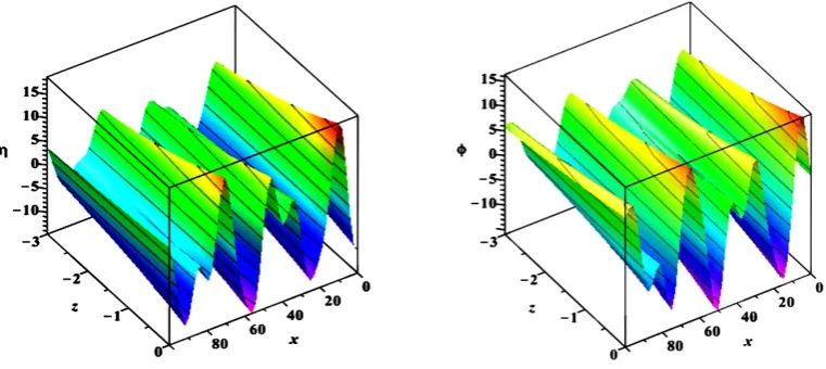
4π, 12π, 60π, 420π, 4620π, 60060π, 1021020π. (145) The KEF structures of conjugate harmonic solutions are visualized in Figure 2 by instantaneous 3d surface plots with isocurves for η
( )
83 and φ( )
84 , for N=3; ρ =n 1 2,1 3,1 5; Cxn =1, 2, 3; Xan=3, 2,1;1.2,1.4,1.6;
n
Fw = and Gwn =1.1,1.3,1.5 at t=114.2. In two dimensions, the pseudovector potential coin-cides with the stream function and isocurves of η coincides with streamlines [2].
The DEF and KEF-DEF structures are visualized in Figure 3 by instantaneous 3d surface plots with isocurves
[image:14.595.142.456.82.167.2] [image:14.595.123.504.532.702.2]
Figure 3. Kinetic energy (left) and dynamic pressure (right) of the lower cumulative flow.
for ke
( )
132 and pd =g zz +(
pt−p0)
ρ, where pt is given by (133), for N =3; ρ =n 1 2,1 3,1 5;1, 2, 3;
n
Cx = Xan=3, 2,1; Fwn=1.2,1.4,1.6; and Gwn=1.1,1.3,1.5 at t=114.2. In agreement with the
Bernoulli Equation [1], local maximums of the DEF structure for ke correspond to local minimums of the
KEF-DEF structure for pd.
The rate of vanishing of the DEF structure is larger than that of the KEF structure. Animations of η ϕ, ,ke, andpd show a transitional behavior of these variables that approach a deterministic chaos, which is determined
by 5N parameters: ρn,Cx Xa Fwn, n, n, and Gwn, as N→ ∞.
5. Conclusions
The analytical methods of undetermined coefficients and separation of variables are extended by the computa-tional method of solving 2d PDEs by decomposition in invariant structures. The method is developed by the ex-perimental computing with lists of equations and expressions and the theoretical computing with symbolic gen-eral terms. The experimental computing of the kinematic and dynamic problems is implemented by 48 proce-dures of 1142 code lines and the theoretical computing by 41 proceproce-dures of 996 code lines.
To compute the upper and cumulative flows for nonlinear interaction of N internal waves in the KF
tures, the KEF, DEF, and KEF-DEF structures were treated both experimentally and theoretically. These struc-tures with constant and space-dependent structural coefficients are invariant with respect to various differential and algebraic operations. The structures continue the Fourier series for linear and nonlinear problems with solu-tions vanishing at infinity and model flows of a deterministic wave chaos with the period that approaches infini-ty.
The exact solutions of the Navier-Stokes PDEs for the nonlinear interaction of N conservative waves are
computed in the upper and lower domains by formulating and solving the Dirichlet problem for the vorticity, continuity, Helmholtz, Lamb-Helmholtz, and Bernoulli equations. The conservative waves are not affected by dissipation since they are derived in the class of flows with the harmonic velocity field. The harmonic relation-ships between fluid-dynamic variables and their spatial derivatives with respect to x both for upper and lower
flows are obtained.
Acknowledgements
The author thanks S. P. Bhavaraju for the stimulating discussion at the 2013 SIAM Annual Meeting. Support of the College of Mount Saint Vincent and CAAM is gratefully acknowledged.
References
[1] Lamb, S.H. (1945) Hydrodynamics.6th Edition, Dover Publications, New York.
[3] Miroshnikov, V.A. (2005) The Boussinesq-Rayleigh Series for Two-Dimensional Flows Away from Boundaries. Ap-plied Mathematics Research Express, 2005, 183-227. http://dx.doi.org/10.1155/amrx.2005.183
[4] Korn, G.A. and Korn, T.A. (2000) Mathematical Handbook for Scientists and Engineers: Definitions, Theorems, and Formulas for Reference and Review. 2nd Revised Edition, Dover Publications, New York.
[5] Kochin, N.E., Kibel, I.A. and Roze, N.V. (1964) Theoretical Hydromechanics. John Wiley & Sons Ltd., Chichester.
[6] Miroshnikov, V.A. (2009) Spatiotemporal Cascades of Exposed and Hidden Perturbations of the Couette Flow. Ad-vances and Applications in Fluid Dynamics, 6, 141-165.