Evolutionary Algorithm for Solving Multi-Mode Resource
Constrained Project Scheduling Problems through
Deterministic Mode Selection
Shivam Agarwal
B. Tech Student, Department of Information Technology
Fr C R college of Engineering Mumbai India 400050
Tushar Bhat
B. Tech Student, Department of Information Technology
Fr C R college of Engineering Mumbai India 400050
ABSTRACT
This work describes a novel approach towards solving Multimode Resource Constrained Project Scheduling (MRCPS) Problems and an algorithm developed to implement this approach. The algorithm is intended to be used as an alternative to the various genetic algorithms currently being used to solve such problems. Using a deterministic approach that aims to select the optimum modes for execution as efficiently as possible, this algorithm has given deviations far below those of previous efforts in J30 dataset as published by PSPLib. This algorithm is expected to have great implications in the field of Optimisation.
General Terms
Project scheduling, evolutionary algorithm, deterministic mode selection.
Keywords
Resource constraints, project scheduling, evolutionary algorithm.
1.
INTRODUCTION
A project scheduling problem consists of n + 2 activities where each activity has to be processed in order to complete the project. Fictitious activities 1 and n+2 correspond to the project start and to the project end, respectively. The activities are interrelated by precedence constraints which force an activity to not be started until all its immediate predecessor activities, as defined in the problem, have been finished.
The Resource Constrained Project Scheduling Problem (RCPSP) is a general scheduling problem which consists of scheduling a set of activities, taking into account temporal and resource constraints. Preemption is not allowed.
A Multi-Mode Resource Constrained Project Scheduling Problem (MRCPSP) can be defined as a set of jobs which need to be performed based on certain constraints. A single project consists of a set of n activities which have to be processed. Each activity has precedence constraints, namely other jobs that need to be completed before the activity can be performed. A source activity (Activity 1) and a sink activity (Activity n + 2) are used to represent project start and end respectively.
Activities are also constrained by m resources, which may be renewable or non-renewable. Renewable resources are replenished upon completion of activity. They represent resources such as manpower, available workstations etc.
which are only used by activities as long as they are being executed and not consumed. Non-renewable resources are used up by activities and are not replenished. They represent exhaustible resources like money, fuel etc. Each activity also has k modes, each mode being a method by which to complete the activity which differs from other modes in duration of completion and amount of resources consumed.
2.
LITERATURE REVIEW
Multiple efforts have been made at solving MRCPS Problems. Optimal solutions have been found for problems which consist of 20 jobs or less using exact algorithms such as [1]-[3]. However, the complexity of MRCPS Problems increases drastically as number of jobs increase. Exact algorithms to find optimum solutions for j30 sums do not exist or are unfeasible due to the large computational complexity involved. Thus heuristic or meta-heuristic approaches are required, such as Genetic Algorithms (GA), which are capable of locating solutions even with a large solution space. A Genetic Algorithm (GA) is a search heuristic that attempts to imitate the process of evolution. Genetic algorithms belong to the larger class of evolutionary algorithms (EA), which generate solutions to optimization problems using techniques inspired by natural evolution, such as inheritance, mutation, selection, and crossover.
Basic GA are used in works such as [4] and [5] to find heuristic solutions for j30 sums, generally by optimising schedule generation after stochastic selection of modes, after ensuring that all constraints are being adhered to. Better results have also been obtained by applying local search optimization techniques such as Particle Swarm Optimisation and Simulated Annealing, as described in [6] and [7] respectively.
3.
PROBLEM DESCRIPTION
For MRCPS Problems with 3 modes and 30 jobs, assuming linear execution of jobs there exists 3^30 possible paths to achieve completion of jobs in every problem (assuming sufficient non-renewable resources), each of which must be analysed to find optimum set of modes to minimise makespan.
is known and can be termed as NP-Hard since they can be solved in polynomial time by a hypothetical oracle machine i.e. it is polynomial time Turing-reducible.
The problem of allocating scarce resources over time to perform a given set of activities – that is, project scheduling - appears in a vast spectrum of real-world situations. Over the last forty years project scheduling problems have been carefully studied, resulting in a considerable body of knowledge. Recently, however, the increase in the power and ubiquity of the computer has had a pronounced effect on research in project scheduling and project scheduling models. As a result, considerable progress has been made in all directions of modeling and finding solutions to these problems.
Our approach towards solving these problems is analytical in nature. It is deterministic in mode selection and is stochastic in sequence selection with adherence to multiple constraints making it only partially stochastic. Our algorithm, first, closely inspects and defines the limits and facets of the MRCPSP and then proceeds with iterative mode selection. This initial algorithm returns multiple possible results which are then further refined and optimised. The final optimised set of selected modes is run through a semi-stochastic sequence selection algorithm which runs multiple iterations to obtain optimum makespan. Our objective is to minimise makespan as far as possible.
4.
ALGORITHM
The work implements a novel approach in solving such problems to select optimal modes and the appropriate schedule or sequence to execute activities in order to achieve, possibly, lowest make span for the entire job. In this work we have selected a set of problems (j30) with the following parameters from well-known project scheduling problem library PSPLib [8]:
Number of total jobs in the set: 640
Number of feasible jobs: 552
Number of activities per job: 30
Number of modes per activity: 3
Number of types of renewable resources: 2
Number of types of non-renewable resources: 2
In our approach, each problem is put through an analytical process designed to systematically select the best possible mode, using which the optimum makespan is expected to be found. It involves selecting the ideal mode based on the relative impact of duration and non-renewable resources on the final makespan. The impact is measured and iteratively changed based on the result of the previous iteration. The results of this step are refined based on the renewable resources available and then further optimised based on leftover non-renewable resources.
The overall algorithm can be represented as follows:
Step 1: Initialise all required variables and arrays
Step 2: Call the necessary function to populate input arrays and variables with input data.
Step 3: Call function to calculate score for each mode of each job.
Step 4: Run initial mode selection algorithm based on current scores. This algorithm selects the best mode according to score and runs it as soon as modes have sufficient renewable resources to run and have satisfied predecessor constraints.
Step 5: Based on success of above process, increment weights and return to step 3 for n number of iterations.
Step 6: If one or more successful set of modes have been found, call the function to refine them to give more successful sets.
Step 7: Send above sets to optimising function, which ultimately returns the final answer after deterministic mode alteration and semi-stochastic sequence selection.
The algorithm can be roughly divided into 4 phases: Analysis, Mode Selection, Refinement, and Optimisation.
4.1
Analysis Phase:
This is the initial phase, consisting of input and preliminary analysis. Data is extracted from problem files and stored. The boundaries of resource parameters are found for scaling purposes.
The purpose of the analysis phase is to find ranges of non-renewable and non-renewable resource consumption per job. These values, along with the values of available resources at time of selection are used to determine which jobs are to be executed and when.
First, of all, a problem set is read and the values of different entities are extracted to populate the class. This has been achieved by using standard MRCPS Problems downloaded from psplib. Minimum and maximum of each parameter is found. This is used for scaling down the value of each parameter.
4.2
Mode Selection:
In this phase, an initial set of weights are given to duration and non-renewable resources. In successive iterations, these weights are used to calculate a score for each mode, on the basis of which a single mode is selected per job. Using these modes, a schedule is generated for all jobs in that problem using a sequencing algorithm. Based on the feasibility of this sequence (which depends mainly on non-renewable resources) the weights are changed and the next iteration is begun. A set number of iterations are run, which result in a proportionate number of unique feasible solutions.
Each mode is given a score by scaling each parameter down and multiplying it by appropriate weight.
Eg. Problem selected: 64_9
Duration Weight (dwt): 2 N1 Weight (n1wt): 1 N2 Weight (n2wt): 1
maxD = maximum duration of all modes for the current problem instance
maxN1 = maximum N1 resource requirement among all modes for the current problem instance
maxN2 = maximum N1 resource requirement among all modes for the current problem instance
Job Mode Duration R1 R2 N1 N2 Score
3 1 5 9 6 7 6 1.844
2 10 4 6 4 3 2.144
3 10 3 1 5 3 2.533
Depending on the score, the jobs are executed on a day to day basis as per availability while being consistent with resource constraints and following predecessor-successor constraints as well. If all the jobs are executed successfully, then the weight of duration is increased in the next iteration, so as to increase the chances of selecting a better mode with lower duration which may give an overall lower duration.
However, if the execution fails in between because of depletion of non-renewable resources, the weights of appropriate resources are increased in the next iteration so as to use fewer resources and ensure that all the jobs get executed.
The modes of the best solutions along with their make span and left-over non-renewable resources are stored for further refinement and optimisation. A redundancy check is also performed to store only unique solutions.
Eg.- After being called 2 times, contents of the array storing solution sets (where each solution set contains list of modes selected per job and duration, n1, n2 details) are:
Duration: 38
0 2 2 1 2 1 2 1 1 1 2 3 1 1 1 1 3 3 3 2 2 2 3 2 1 1 2 1 3 1 3 0
N1: 33 N2: 30
Duration: 34
0 1 1 1 2 1 2 1 1 1 1 2 1 1 1 1 1 1 3 2 1 2 1 1 1 1 2 1 2 1 3 0
N1: 16 N2: 14
After being called 4 times contents of array storing solution sets are:
Duration: 38
0 2 2 1 2 1 2 1 1 1 2 3 1 1 1 1 3 3 3 2 2 2 3 2 1 1 2 1 3 1 3 0
N1: 33 N2: 30
Duration: 34
0 1 1 1 2 1 2 1 1 1 1 2 1 1 1 1 1 1 3 2 1 2 1 1 1 1 2 1 2 1 3 0
N1:16 N2: 14
Duration: 33
0 1 1 1 2 1 2 1 1 1 1 2 1 1 1 1 1 1 3 1 1 1 1 1 1 1 2 1 2 1 1 0
N1: 13 N2: 11
Duration: 32
0 1 1 1 2 1 2 1 1 1 1 1 1 1 1 1 1 1 3 1 1 1 1 1 1 1 2 1 2 1 1 0
N1: 12 N2: 9
4.3
Refinement:
In this phase, modes are changed in those cases where a different mode has the same duration as the selected mode, but has better renewable resource requirements and does not differ too much in terms of non-renewable resource requirements. The new set of modes is stored as a separate solution set since it too is a feasible set. The purpose of this phase is to increase the number of solution sets in order to increase the possibility of obtaining the optimum makespan.
If the duration of two modes in a job are same, then the mode which uses less renewable resources is selected, given there are enough left-over non-renewable resources left to permit such a change in stored solutions. The newly generated solution is stored along with the original set for further optimisation after a redundancy check to ensure that only unique solutions are being stored.
Eg.- the contents of the array storing solution sets (where each solution set contains the list of modes selected per job, duration and the remaining n1, n2) before calling refine function, are:
Duration: 38
0 2 2 1 2 1 2 1 1 1 2 3 1 1 1 1 3 3 3 2 2 2 3 2 1 1 2 1 3 1 3 0
N1: 33 N2: 30
Duration: 34
0 1 1 1 2 1 2 1 1 1 1 2 1 1 1 1 1 1 3 2 1 2 1 1 1 1 2 1 2 1 3 0
N1: 16 N2: 14
Duration: 33
0 1 1 1 2 1 2 1 1 1 1 2 1 1 1 1 1 1 3 1 1 1 1 1 1 1 2 1 2 1 1 0
Duration: 32
0 1 1 1 2 1 2 1 1 1 1 1 1 1 1 1 1 1 3 1 1 1 1 1 1 1 2 1 2 1 1 0
N1: 12 N2: 9
Duration: 31
0 1 1 1 2 1 2 1 1 1 1 1 1 1 1 1 1 1 1 1 1 1 1 1 1 1 2 1 2 1 1 0
N1: 7 N2: 9
Duration: 31
0 1 1 1 1 1 2 1 1 1 1 1 1 1 1 1 1 1 1 1 1 1 1 1 1 1 2 1 2 1 1 0
N1: 4 N2: 6
The new solution sets added to the array after calling refine function two times are:
Duration: 38
0 2 3 1 2 1 2 1 1 1 2 3 1 1 1 1 3 3 3 2 2 2 3 2 1 1 2 1 3 1 3 0
N1: 32 N2: 30
Duration: 38
0 2 2 1 2 1 1 1 1 1 2 3 1 1 1 1 3 3 3 2 2 2 3 2 1 1 2 1 3 1 3 0
N1: 33 N2: 28
4.4
Optimisation:
This is the final phase of this algorithm. In this phase, each solution set is put through a stochastic schedule generating algorithm. This algorithm uses the selected modes, and based on predecessor-successor constraints and renewable resource constraints, randomly selects jobs to be executed, out of a pool of available jobs, on a day to day basis. This algorithm is run for a set number of iterations for each solution set to ensure that the best possible sequence is selected. The best makespan is selected and stored for output and analysis purposes. Furthermore, after the initial set of solution sets are sequenced, each solution set is optimised iteratively, by reducing the mode of one job and increasing the modes of other jobs to compensate for the excess requirement of non-
renewable resources. The purpose of this is to give more optimal solution sets, each of which are then put through the sequencing to obtain their makespan. This optimisation
process is continued for a set number of iterations, for which makespans are recorded if they show improvement over previous iterations. At the end of this phase, the best possible makespan found so far is recorded as the final solution given by this algorithm for that particular problem.
Pseudo Code:
Step 1: Given a solution set, begin sequencing process by initialising clock or day-counter.
Step 2: Based on predecessor constraints, create set of available jobs each day.
Step 3: Randomly select which jobs, out of all the available ones, are to be executed based on currently available renewable resources. In case of insufficient resources to begin executing all jobs, randomly select jobs until resources are insufficient.
Step 4: Repeat steps 1 to 3 for n iterations to find (semi-stochastically) the lowest makespan for the current set of modes.
Step 5: For the current set of modes, select one job for which mode can be reduced with highest possible gain in duration.
Step 6: Continually increase modes for other jobs, in order of increasing loss of duration, until the difference in non-renewable resources caused by reducing the above job's mode is balanced.
Step 7: For this new set of modes, repeat steps 1 to 4.
Step 8: Repeat steps 5 to 7 for n number of iterations.
Step 9: Repeat steps 1 to 8 for each set of modes available after performing refining process.
Eg.- Stored modes of selected solution set before optimise function is called:
2, 2, 1, 2, 1, 2, 1, 1, 1, 2, 3, 1, 1, 1, 1, 3, 3, 3, 2, 2, 2, 3, 2, 1, 1, 2, 1, 3, 1, 3
Changed modes of selected solution set after optimise function is called 15 times:
1, 1, 1, 2, 1, 2, 1, 1, 1, 1, 1, 1, 1, 1, 1, 1, 3, 3, 1, 1, 1, 1, 1, 1, 1, 2, 1, 2, 1, 3
5.
RESULT ANALYSIS
Table 1. Percentage deviations obtained by implementing stages separately
Iterative Mode Selection
Stochastic Schedule Generation
Refinement Phase
Optimisation Phase
Proposed Algorithm
Mode Selection Yes Yes Yes Yes Yes
Random Schedule Yes Yes Yes Yes
Refinement Yes Yes
Optimisation Yes Yes
Random Iterations N/A 200 200 200 200
Deviation Obtained 13.962 10.41 9.79 9.68 7.87
The table given above shows the deviation from best known solutions obtained by executing variations of the algorithm to analyse the effects of separate phases on the results obtained.
i) It is seen that a sharp decrease in deviation is obtained upon implementing stochastic schedule generation. This shows that with optimum mode selection, the probability of obtaining optimum schedule through stochastic selection becomes very high.
[image:5.595.54.281.468.583.2]ii) Implementation of Optimisation and Refinement phases separately does not cause much difference in results but the combined implementation of all the phases shows another sharp decrease in the resultant deviation. Upon analysis it is seen that successive operation of the phases generates more and better solution sets which are more likely to have optimum solutions.
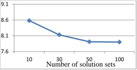
Figure 2 % deviation obtained by varying number of unique solution sets stored
The above graph shows the variation in results obtained by changing the number of unique solution sets stored by the algorithm. The number of stochastic schedule generating iterations is 100. These solution sets are generated and processed by the various phases and in order to find optimum modes, thus the number of solution sets stored has a large impact upon the final deviation obtained. Since increasing the number of solution sets stored drastically increases computation time, it was decided to store 50 solution sets in the final algorithm since increasing this number to the next amount has given a negligible decrease in deviation.
Figure 2 % deviation obtained by varying number of stochastic schedules generated
[image:5.595.309.552.542.612.2]The above graph shows the variation in results obtained by changing the number of stochastic iterations used to generate schedules for 50 solution sets. While the increase in iterations run shows a corresponding decrease in deviation, the computational time taken increases drastically with increase in number of iterations. Thus, an optimum balance is struck between deviation and time taken at 200 iterations.
Table 2 Average deviation from the best known solutions available
Jozefowska et. al. (2001) [7]
Lova et. al. (2009) [9]
Bilolikar et. al. (2011) [10]
This work
11.67 16.65 11.86 7.87
Table 3 Average deviation from the critical path lower bound
Talbot et. al. (1982) [1]
Grunewald et. al. (1993) [11]
Kolisch et. al. (1997) [12]
This work
28.07 26.52 30.87 22.30
As seen in the above tables, the deviation obtained from the known optimal solutions given by our algorithm is a large improvement over the deviation of previous works on the same problem set by others.
7.6 8.1 8.6 9.1
10 30 50 100
Number of solution sets
7.8 7.9 8 8.1
50 100 200 500
6.
CONCLUSION
In this work, an evolutionary algorithm has been presented. This algorithm has been used to solve multi-mode resource-constrained project scheduling problems. The proposed evolutionary algorithm proves its effectiveness as problem solving technique for the MRCPSP by generating competitive results for the j30 PSPLIB dataset. Research indicates that deterministic mode selection through the use of careful analysis and logical rule selection is highly useful in obtaining optimum results. Accuracy of results may be improved by applying local search optimization techniques to the results obtained so far
7.
ACKNOWLEDGMENTS
Our thanks to Prof. Mahesh R. Sharma for his guidance and help, without which this research would not have been possible.
8.
REFERENCES
[1] Talbot, F.B., 1982. Resource-constrained project scheduling with time-resource trade-offs: the non-preemptive case. Management Science 28 (10), 1197– 1210
[2] Patterson, J.H., Słowin´ ski, R., Talbot, F.B., We˛glarz, J., 1989. An algorithm for a general class of precedence and resource constrained scheduling problems. In: Słowin´ ski, R., Weglarz, J. (Eds.), Advances in Project Scheduling. Elsevier, Amsterdam, pp. 3–28.
[3] Sprecher, A., 1994. Resource-constrained project scheduling: exact methods for the multi-mode case. Springer, Berlin
[4] M.B. Wall,"A Genetic Algorithm for Resource-Constrained Scheduling", Dept. of Mech. Engg., M.I.T., June 1996.
[5] Alcaraz, J., Maroto, C., Ruiz, R. Solving the multi-mode resource-constrained project scheduling problem with genetic algorithms. Journal of the Operational Research Society, 54(6):614626, 2003.
[6] M. Higashitani, A. Ishigame and K. Yasuda, Particle Swarm Optimization Considering the Concept of Predator-Prey Behavior ",IEEE Congress on Evolutionary Computation, July 2006.
[7] Jozefowska, J., Mika, M., Rozycki, R., Waligora, G., Weglarz, J. Simulated annealing for multimode resource-constrained project scheduling. Annals of Operations Research, 102(1):137155, 2001.
[8] Project Scheduling Problem Library PSPLib: http://129.187.106.231/psplib/.
[9] Lova, A., Tormos, P., Cervantes, M., Barber, F. An efficient hybrid genetic algorithm for scheduling projects with resource constraints and multiple execution modes. International Journal of Production Economics, 117(2):302 316, 2009
[10] Bilolikar, V. S., Jain, K., Sharma, M. R., An Annealed Genetic Algorithm for Multi Mode Resource Constrained Project Scheduling Problem, International Journal of Computer Applications (0975 – 8887) Volume 60– No.1, December 2012
[11] Drexl, A., Gruenewald, J. Nonpreemptive multi-mode resource-constrained project scheduling. IIE transactions, 25(5):7481, 1993
[12] Kolisch, R., Drexl, A. Local search for nonpreemptive multi-mode resource-constrained project scheduling. IIE transactions, 29(11):987999, 1997