Human Face Recognition using Stationary Multiwavelet Transform

Volume 72– No.1, May 2013

Human Face Recognition using Stationary

Multiwavelet Transform

Tarik Z. Ismaeel,Ph.D

University of Baghdad College of Engineering, Electrical Engineering Department.

Aya A. Kamil

University of Baghdad College of Engineering,

Electrical Engineering Department.

Ahkam K. Naji

Ministry of Higher Education and Scientific Research.

Abstract

Face recognition is a complex visual classification task which plays an important role in computer vision, image processing, and pattern recognition. SMWT is proposed to extract the features in images before using the PCA and histogram based method classifiers. SMWT will be used in the recognition process to minimize the size of the data base. Since left direction poses equal to the right direction poses, and as it is a translation invariant, so it has the same data, so one can delete some images that have such direction in poses, so the size of the database will reduce. Also SMWT will be used to enhance the recognition rate. In this approach the recognition rate was94.5%byusing the Histogram Based Method, and a 63% when using (PCA), when the numbers of training and test images are both equal five images.

Index Terms—Face Recognition, Stationary Wavelet

Transform (SWT), Stationary Multiwavelet Transform (SMWT), Histogram Based Method, Principle Component Analyses.

1. INTRODUCTION.

Security is the one of the main concern in today’s world. Whether it is the field of telecommunication, information, network, data security, airport or home security, national security or human security, there are various techniques for the security. Biometric is one of the modes of it. Face recognition is one of the various biometric techniques used in identifying humans. Biometrics use physical and behavioral properties of the human. All biometric systems need some records in database against which they can search for matches. Biometrics being investigated includes fingerprints, speech, signature dynamics and face recognition [1]. Face plays a primary role in identifying the person and

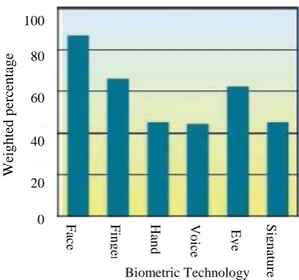
also face is the more easily recognizable part of the human. As thousands of faces can be recognized in lifetime, this skill is very robust because a person can be identified even after so many years with different aging, different lightening conditions and viewing conditions [2]. Face recognition is one of the highly used biometric techniques [3] as shown in figure (1).

Figure (1) Comparison among various biometric techniques. Researchers are trying to implement robust face recognition systems, similar to the human recognition capabilities under various conditions, for security and multimedia information access applications where the identification of the subject is necessary. The task of machine recognition of humans is becoming increasingly difficult and complex as both of the conditions constrains and the sample sizes are growing. Face recognition has received substantial attention from researchers in biometrics, pattern recognition, and computer vision communities [4].

Face recognition appears to offer several advantages over other biometric methods, a few of which are outlined below:

Face F

in

g

er

Han

d

Vo

ice Ey_e

Sig

n

atu

re

Wei

ght

ed per

cent

age

100

80

60

40

20

0

Volume 72– No.1, May 2013

Almost all these technologies require some voluntary action by the user, i.e., the user needs to place his hand on a hand-rest for fingerprinting or hand geometry detection and has to stand in a fixed position in front of a camera for iris or retina identification. However, face recognition can be done passively without any explicit action or participation on the part of the user since face images can be acquired from a distance by a camera. Technologies that require multiple individuals to use the same equipment to capture their biological characteristics potentially expose the user to the transmission of germs and impurities from other users. However, face recognition is nonintrusive and does not carry any such health risks [5].

2. Stationary Wavelet Transform

The stationary Wavelet transform (SWT) was proposed by Nason and Silverman [6], which is redundant, shift invariant, and it gives a denser approximation to the continuous Wavelet transform than the approximation provided by the orthogonal wavelet transform, it is also called undecimated Wavelet transform.

The DWT lacks translation invariance [7-9] while the SWT expands the amount of data by over-representing signals in the Wavelet domain. The two main discrete Wavelet methods are known generally as the DWT and the SWT. Both methods use a mother Wavelet, []

which can be translated and dilated according to equation (1).



j,k(x)=

2



(

2

𝑥 − 𝑘)

(1)

Equations (2) and (3) describe the DWT decomposition process. The broad scale, or approximation, coefficients

𝑎𝑗𝐷𝑊𝑇 are convolved separately with 𝑔0 and ℎ0and the

result is down-sampled by two. This process splits the

𝑎𝑗𝐷𝑊𝑇frequency information roughly in half, partitioning

it into a set of fine scale, or detail coefficients 𝑑𝑗 +1𝐷𝑊𝑇and a

coarser set of approximation coefficients𝑎𝑗 +1𝐷𝑊𝑇. This

procedure can be iteratively continued until the desired level of decomposition, j= J, is obtained.

𝑎

_{𝑘 = ℎ}

𝑛

𝑛 − 2𝑘 𝑎

𝑘

(2)

𝑑

_{𝑘 = 𝑔}

𝑛

𝑛 − 2𝑘 𝑎

𝑘

(3)

Down-sampling the DWT coefficients between each level acts to halve their effective sample frequency and halve the effective corner frequencies of theh0andg0

filters for the next level of processing. Therefore, identical filters can be used for each step of the DWT procedure.

Dyadically down-sampling the approximation and detail coefficients from f(n) leads to a completely different set of DWT coefficients than down-sampling the coefficients from its shifted version, f(n+1). Similarly, choosing to retain the odd Wavelet coefficients during the dyadic down-sampling will result in a different outcome than retaining the even Wavelet coefficients [7– 9]. As a result of the shift variability of the DWT, several authors have used translation invariant decomposition

techniques, such as the continuous Wavelet transform or SWT.

In contrast to the DWT, the SWT up samples the decomposition filters by inserting zeros between every other filter coefficient and, consequently, avoids the translational variance problem caused by decimation [10]. The absence of a decimator leads to a full rate decomposition. Each sub band contains the same number of samples as the input [11]. Therefore, the SWT uses a set of level dependent decomposition filters,ℎ𝑖 and 𝑔𝑖,

which are theh0andg0 filters with 2j-1 zeros between each

discrete filter coefficient.

The SWT approximation and detail

coefficients can then be computed using

(2) and (3):

𝑎

_{𝑘 = ℎ}

𝑖

𝑛

𝑛 − 𝑘 𝑎

𝑘 (4)

𝑑

𝑘 = 𝑔

𝑛 − 𝑘 𝑎

𝑘 (5)

The 2D SWT is based on the idea of no decimation [12-13]. It applies the Discrete Wavelet Transform (DWT) and omits both down-sampling in the forward and up-sampling in the inverse transform.

More precisely, it applies the transform at each point of the image and saves the detail coefficients and uses the low frequency information at each level. The Stationary Wavelet Transform decomposition scheme is illustrated in figure (2) where 𝐼𝑖, 𝐺𝑖, 𝐻𝑖are a source image, low-pass

filter and high-pass filter, respectively.

Figure (2). SWT decomposition scheme [12].

3. Stationary Multiwavelet Transforms

(SMWT).

Nason and Silverman made a concept of stationary scalar Wavelet transformation in 1995[6], and they gave out the algorithm of decomposition and reconstruction, which means low-pass filter and high-pass filter are interpolated with zero, and the stationary Wavelet can be decomposed without secondary extraction of the output coefficient of the filters. They also pointed out the stationary Multiwavelet could restrain the fake oscillatory occurrence which exists in the mutation of signal, that is

𝐶𝑗

𝐺𝑗

𝐻𝑗

𝐺𝑗

𝐻

𝐻𝑗

𝐺𝑗 Rows

Rows

Columns

Columns

𝑑𝑒𝑡𝑎𝑖𝑙

Columns

Columns

𝑑𝑒𝑡𝑎𝑖𝑙

Volume 72– No.1, May 2013

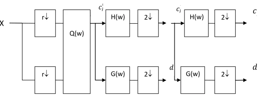
translation invariance. There are differences in the decomposition process of 2D images of stationary Multiwavelet transformation and general multi Wavelet transformation. Figure (3) is a traditional Multiwavelet decomposition chart. Figure (4) is a decomposition chart of stationary Multiwavelet transformation of 2D image. As it can be seen through it, after low-pass and high-pass filtering, each decomposition level of stationary Multiwavelet doesn’t have any secondary extraction, so after a layer of decomposition the first level approximation and detailed coefficient matrix are the same size as data matrix of input image after having been preprocessed, rather than the half step by step.

Low-pass and high-pass filter of the later decomposition level of Stationary Multiwavelet transformation are the results of the former decomposition level after matrix interpolated with zero. Matrix interpolated with zero means interpolating an r r zero matrix. Because stationary multiwavelet inputs an r-dimension data and the coefficients of filter is a matrix, each operation interpolated with zero must interpolate an r r matrix. In figure (4) Hj , Gj are the results of H and G with j time’s operation of matrix interpolated with zero.

The following figure (5) is the chart of matrix interpolated with zero operation.

Figure (3) Structure chart of simple multi-Wavelet transform

.

Figure (4) Structure chart of stationary multi-Wavelet transform.

Figure (5) Matrix interpolated with zero.

4. Principal Component Analysis.

The Principal Component Analysis (PCA) is one of the most successful techniques that have been used in image recognition and compression [14].

The purpose of PCA is to reduce the large dimensionality of the data space (observed variables) to the smaller intrinsic dimensionality of feature space (independent variables), which are needed to describe the data economically. This is the case when there is a strong correlation between observed variables. The jobs which PCA can do are prediction, redundancy removal, feature extraction, data compression, etc. Because PCA is a classical technique which can do something in the linear domain, applications having linear models are suitable, such as signal processing, image processing, system and control theory, communications, etc. [14].

The main idea of using PCA for face recognition is to express the large 1-D vector of pixels constructed from 2-D facial image into the compact principal components of the feature space. This can be called Eigen space projection. Eigen space is calculated by identifying the eigenvectors of the covariance matrix derived from a set of facial images (vectors) [15].

𝐻

2

↑

_𝐻

_𝐺

2

↑

_𝐺

𝐶𝑗

𝐺𝑗

𝐻𝑗

𝐺𝑗

𝐻

𝐻𝑗

𝐺𝑗 Rows

Rows

Columns

Columns

𝐷_ℎ𝑗 +1𝑑𝑒𝑡𝑎𝑖𝑙

Columns

Columns

𝐶𝑗 +1_{𝑎𝑝𝑝𝑟𝑜𝑥.}

𝐷𝑣𝑗 +1𝑑𝑒𝑡𝑎𝑖𝑙

𝐷_𝑑𝑗 +1𝑑𝑒𝑡𝑎𝑖𝑙

X

r



r



2



2



2



2



Q(w)

H(w)

G(w)

H(w)

G(w)

𝑐

𝑐

_{. . ….}

𝑑

𝑐

Volume 72– No.1, May 2013

5. Histogram Based Methods.

Recognizing objects from large image databases by using histogram based methods have proved simplicity and usefulness in last decade. Initially, this idea was based on color histograms that were launched by Swain and Ballard [16].

Histogram or Frequency Histogram is a bar graph. The horizontal axis depicts the range and scale of observations involved and vertical axis shows the number of data points (pixels) in various intervals, i.e. the frequency of observations in the intervals. Histograms are popular among statisticians. Though they do not show the exact values of the data points they give a very good idea about the spread of the data and shape. Histogram analysis is a popular method used in the image retrieval field. Histograms are invariant to translation and rotation about an axis perpendicular to the image plane, and change only slowly under change of angle of view, change in scale and occlusion. Because histograms change slowly with view, an object can be adequately represented by a small number of histograms, corresponding to a set of canonical views [17].

6. The Proposed Face Recognition

System Block Diagram.

The general structure of the proposed face recognition system is shown in Figure (6). Function of each block is clarified below:



the effect of lightning source amplitude’s variations. Feature Extraction: SWT is used to split the images into four sub image at low resolution, but in the same dimension of the original images, not like the scalar wavelet, where the images is quadratic of the original images. And the SMWT split the images into four sub image just in the LL part as shown in figure (7).

Classifier: two techniques are used here. These are classifiers that were used in this research with a brief description of each one.

Figure (7).The SMWT applied on image.

7. Histogram based methods Classifier.

The histogram of an image shows the statistical distribution of pixel intensities, which can be considered as a feature vector representing the image in lower dimensional space. In a general mathematical sense, an image histogram is simply a mapping _𝑖 that counts the number of pixel intensity levels that fall into various disjoint intervals, known as bins. The bin size determines the size of the histogram vector. In this paper the bin size is assumed to be 1 and the size of the histogram vector is 256. Given a monochrome image, histogram _𝑖meets the following conditions, where N is the number of pixels in an image.

𝑁 =



𝑖=0

(6)

Then, histogram feature vector, H is

defined by,

H= [



,



, … .



] (7)

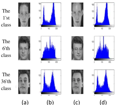
Figure (8) (a) and (c) shows different poses of faces at each row from ORL face database [18]. The histograms of these faces are given in Figure (8) (b) and (d) respectively, which clearly illustrates that the histograms in the same classes are highly correlated, which is not the case for the histograms of faces from different classes.

Figure (8) Face images of different classes with their corresponding gray level histograms.

The gray level histogram of the entire face image is used as the face descriptor of a given face. The proposed face recognition system simply uses gray level histograms to

SMWT

Preprocessing _{Normalization}

Feature

Extraction Classifier

Face is recognized as one of the faces in the database or as unknown faces

Tested Human face

Images

Figure (6) The Proposed Face Recognition System Block Diagram.

The 1'st class

The 6'th class

The 36'th class

(

Volume 72– No.1, May 2013

describe faces and recognition is achieved by incorporating histogram matching method between the histogram of the input face and the histograms of the faces in the training set.

For training phase, gray scale images with 256 gray levels are used. Firstly, frequency of every gray-level is computed and stored in vectors for further processing. Secondly, the mean of consecutive nine frequencies from the stored vectors is calculated and stored in another vectors for later use in testing phase.

This mean vector is used for calculating the absolute differences among the mean of trained images and the tested image. Finally the minimum difference found identifies the matched class with test image.

Histogram of gray scale image will use 256 bins. Figure (9) shows a sample histogram of the input image. The peak at each bin shows the frequency of that particular bin.

Figure (9) Histogram of an Image.

8. Principal component analysis (PCA)

classifier.

The principal Component Analysis (PCA) is widely used in several applications like signal processing and image compression. It is also called as Karhunen-Loeve transform (KLT).

It uses the covariance or correlation matrix of given data [14]. The PCA is used for multidimensional data set and it is one of the dimensionality reduction (without any information loss) methods. PCA high light the similarities and differences between the variables in the data [15].

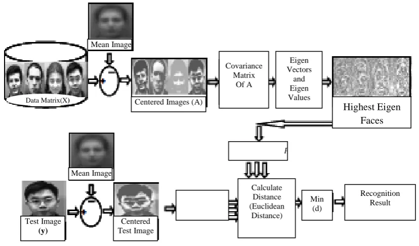
The first step in face recognition system is to calculate the mean vector from the data matrix. The mean vector is then subtracted from all images in the training set. Then training set images are projected into the Eigen space. This resulting vector is small in dimension compared to the data matrix. The given tested image is also subtracted from the mean and is projected into the same former Eigen space. After projecting the images into the Eigen space, the distance measure was used to calculate the recognition rate. In a significant number of literatures the commonly used distance measure is the Euclidean distance measure. A less distance value gives the more recognition rate. This PCA method for face recognition is explained in figure (10). Depending upon the matching result, one can calculate the recognition rate. A high recognition rate gives the best performance.

Figure (10).Principal component analysis algorithms for face recognition.

Covariance Matrix

Of A

Min (d)

Recognition Result Calculate

Distance (Euclidean

Distance)

𝑃𝑦= 𝑊𝑇𝑦

Centered Test Image Test Image

(y)

Mean Image

Data Matrix(X) _{Centered Images (A)}

Mean Image

Eigen Vectors

and Eigen Values

𝑃𝑥= 𝑊𝑇𝑋

Volume 72– No.1, May 2013

9. Experiments on ORL Face database.

Ten different images for each of the 40 distinct subjects were used, for some subjects; the images were taken at different times, varying the lighting condition, facial expressions (open / closed eyes, smiling / not smiling) and facial details (glasses / no glasses). All the images were taken against a dark homogeneous background with the subjects in an upright, frontal position (with tolerance for some side tilting and rotation of up to about 20 degrees. There is some variation in scale of up to about 10%.

Thumbnails of all of the images are shown in figure (11). The images are gray scale with a resolution of 92*112 [18].

Figure (11): The ORL face database. There are 10 images each of the 40 subjects.

10. Experimental Results.

Results of Different Kind of Training

and Test Images.

The results and comparison is made between two methods namely MWT and SMWT.

A. Using Different Number of Training

and Test Images:

Since there are 10 images per individual in the generalized database the effect of different number of training and test image combinations is tested.

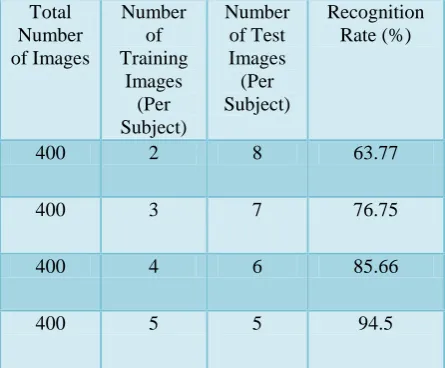
From the tests results in Table (I), it can be seen that using 5 training images and 5 testing images for each individual gives better results; hence, the rest of the tests are conducted using 5 training and 5 test images per individual.

Success rate%= (No. of images correctly recognized÷ Total No. of images in the dataset) × 100.

This result is obtained by using the SMWT with HBM, while the result using the Multiwavelet transform will be shown in table (II).

Table (I).

The success Rates Using Different

Number of Training and Test Images

Using the Histogram Based Method.

Total Number of Images

Number of Training

Images (Per Subject)

Number of Test Images (Per Subject)

Recognition Rate (%)

400 2 8 63.77

400 3 7 76.75

400 4 6 85.66

400 5 5 94.5

Table II. The Success Rates Using

Different Number of Training and Test

Images using the Multiwavelet

transform.

Total Number

Of images

Number of training

images (per subject)

Number of Test images (per subject)

Recognition Rate (%)

400 2 8 60.25

400 3 7 72.75

Volume 72– No.1, May 2013

400 5 5 89.5

B. Changing the Training and Test

Image Combination:

In the second part of the experiments, the effect of changing the images of each individual used in the training and testing stage in a rotating manner has been studied.

From the tests results in Table (III), it can be easily observed that the success rate changes with respect to the utilized sets of training and testing images. Best result that can be achieved is 97.5 % when total number of training samples is 200.

Table III.

The success Rates Using Different

Number of Training and Test Images.

Total Number of Images

Images Used in Training

Images Used in Testing

Recognition Rate (%)

400 1,3,5,7,9 2,4,6,8,10 91

400 1,2,3,4,5 6,7,8,9,10 94.5

400 6,7,8,9,10 1,2,3,4,5 97.5

C. Comparison of Histogram method

with PCA method:

The results of the experiment on ORL database has been shown in Table (IV) and the corresponding graphical representation have been shown in figure (16) from Table (IV), it can be seen that the Histogram approach gives the better recognition rate than PCA approach.

Table IV.

Comparison of Histogram Based

Method with PCA Method.

9 8 7

6 5

Training Samples

90 88.75 78.33

68.75 63

PCA

100 100 100

96.88 94.5

Histogram Based method

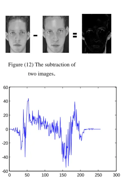
Here the usefulness of the SMWT is shown, where it reduces the size of the database since the SMWT is translation invariant so it can use five, little less or little more images for every person instead of ten images. Let us consider these two images.

If

Figure (13) The difference between the two images. It can be seen that the maximum difference between them it at range (60,-60). But when using the SMWT, the maximum difference between them it at range (25,-25). So it can use just one image instead of three or or four, so as a total of ten images it can use just five images.

0 50 100 150 200 250 300 -60

-40 -20 0 20 40 60

=

_

Volume 72– No.1, May 2013

Figure (14) The difference between the two images after the SMWT.

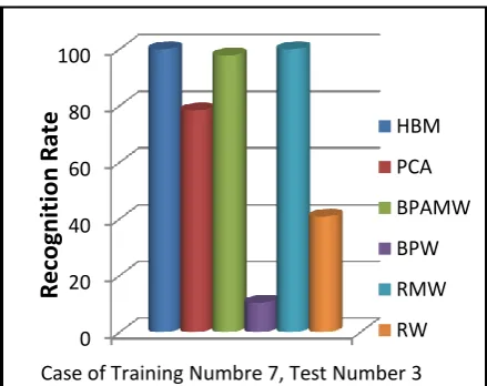
Another comparison is made between the Stationary Multiwavelet Transform (SMWT) and other methods [19] such as, Back Propagation Adaptive Multiwavenet (BPAMW), Back Propagation Wavenet (BPW), Radial Multiwavenet (RMW) and Radial Wavenet (RW). The comparison is made when the number of images in the training set was 7 and 3 in the test set. In this research, the recognition rate was 100% in HBM and 78.33% in PCA, while it was 97.75% in the BPAMW, 10.4167% in the BPW, 100% in the RMW and 40.8333% in the RW as it shown in figure (15).

Figure (15) Comparison between different types of recognition methods.

11. DISCUSSION.

The above system is trained and tested using MATLAB 11.a. For checking the correctness of proposed techniques, ORL (Olivetti Research Laboratory) database was used, which consists of 40 subjects with 10 images per subject, with a total of 40 × 10 = 400 images. Out of 400 images, 200 images were used for training and remaining 200 used for testing purposes.

In table (I) here different numbers of training and test images was used.

It has been shown that as the number of training images (per subject) increases, the recognition rate increases. It can be seen that using 5 training images and 5 testing images for each individual result with better rate. In table (II) the multiwavelet transforms were used. In table (III) it has been shown that the recognition rate changes with changing the style of images distribution. The highest recognition rate is 97.5% when the images are arranged as (6,7,8,9,10) in the training set and (1,2,3,4,5) in the test set. In table (IV) a comparison of histogram based method with PCA method is done, and the recognition rate in histogram based method is higher than that in the PCA method, where it was 100% when the number of image in the training set was 7, while it was 78.33% in the PCA method.

Also it has been shown that the stationary Wavelet transform (SWT) has the benefit of translation invariant, which means that if there is a small difference in the poses of the images taken for every individual (degree of rotation of the face) , so it can be used less number of images to represent a person. Therefore, instead of 10 images to every person, it can be used just 5 images to each individual. So the same results have been obtained here using stationary multiwavelet transform (SMWT), but with smaller size database.

Figure (16) Graphical Representation of Table (IV).

12. CONCLUSIONS.

The face recognition performance has been systematically evaluated by using the AT&T "The Database of Faces" (formerly "The ORL Database of Faces"). The evaluation is based on linear subspace techniques such as the principal component analysis (PCA), and the Histogram based methods. Among these techniques, Histogram based method gives better performance on larger databases when compared to the other technique.

As opposed to conventional PCA Technique, Histogram Based method is proved to be relatively easy and efficient. In PCA approach the image covariance matrices is to be computed but with the use of this approach there is no need to calculate the covariance matrices.

Histogram Based approach leads to large memory requirement due to processing of each image histogram as a result of which speed may decrease but on the other

0 50 100 150 200 250 300

-25 -20 -15 -10 -5 0 5 10 15 20 25

0 20 40 60 80 100

Case of Training Numbre 7, Test Number 3 HBM

PCA

BPAMW

BPW

RMW

RW

R

e

co

gn

iti

on

R

ate

0 50 100

5 _{6 7}

8 ₉

HBM

PCA

R

ec

ognition

Training

Volume 72– No.1, May 2013

hand accuracy level is increased which is an advantage to the system.

In face recognition, there is a need to spatial information in the image to improve recognition rate. The stationary Multiwavelets transform, gives the spatial and frequency information of the images at the same time.

Also, the size of the database was reduced. As the SMWT is a translation invariant, a slightly difference in poses to a certain degree does not affect, so, it can delete some images that have slightly difference in poses. So this is another benefit of the use of the SMWT first the recognition rate is arise and the size of the database is reduce.

Some of the tested images are shown below:

Figure (17) Image of subject 9 matches with image of subject 9.

Figure (18) Image of subject 30 matches with image of subject 30.

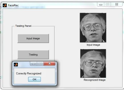
The images of some of the tests in GUI

mode are shown below:

Figure (19) Image of subject 2 matches with image of subject 2.

Figure (20) Image of subject 8 matches with image of subject 8.

13. REFERENCES.

[1] S. Lawrence, C. Lee Giles, A. Chung Tsoi, and A. D. Back,‖ Face Recognition: A Convolutional Neural Network Approach,‖ IEEE Transactions on Neural Networks, Special Issue on Neural Networks and Pattern Recognition.

[2] M. Aleemuddin, ―A Pose Invariant Face Recognition system using Subspace Techniques,‖ Deanship of Graduate studies, 2004.

[3] B. J. Lei, E. A. Hendriks, and M. Reinders, ―On Feature Extraction from Images,‖ Technical Report on MCCWS project, Information and Communication Theory Group TUDelft, 1999. [4] R. Chellappa, C.L. Wilson, and S. Sirohey, ―Human

and machine recognition of faces: A survey,‖ Proc. IEEE, vol. 83, pp. 705–740, 1995.

[5] R. Jafri, and H.R. Arabnia, ―A Survey of Face Recognition Techniques,‖ Journal of Information Processing Systems, Vol. 5, Issue 2, pp. 41-68, June 2009.

[6] G.P. Nason, and B.W. Silverman, "The stationary Wavelet transform and some statistical applications," in: A. Antoniadis, G. Oppenheim (Eds.), Wavelets and Statistics, Springer-Verlag, New York, pp. 281–299, 1995.

[7] M. Lang, H. Guo, J. E. Odegard, C. S. Burrus, and R.O. Wells, ―Noise reduction using an undecimated discrete Wavelet transform,‖ IEEE Signal Process. Letters, vol. 3, no. 1, pp. 10–12, Oct. 1995.

[8] J. Liang, and T. W. Parks, ―A translation-invariant Wavelet representation algorithm with applications,‖ IEEE Trans. Signal Process. vol. 44, no. 2, pp. 225–232, Feb. 1996.

[9] J. Pesquet, H. Krim, and H. Carfantan, ―Time-invariant orthonormal Wavelet representations,‖ IEEE Trans. Signal Process., vol. 44, no. 8, pp. 1964–1970, Aug. 1996.

[10] S. Mallat, ―Zero-Crossings of a Wavelet transform,‖ IEEE Trans. Inf.Theory, vol. 37, no. 4, pp. 1019– 1033, Jul. 1991.

Volume 72– No.1, May 2013

[12] Q. Gao, Y. Zhao and Y. Lu, ―Despecking SAR image using stationary Wavelet transform combining with directional filter banks,‖ Applied Mathematics and Computation, vol. 205, pp. 517– 524, 2008.

[13] G. Pajares and J. Manuel la Cruz, ―A Wavelet-based image fusion tutorial,‖ Pattern Recognition, pp. 1855–1872, 2004.

[14] M. Kirby and L. Sirovich, ―Application of the karhunen-loeve procedure for the characterization of human faces,‖ IEEE Trans. Pattern Analysis and Machine Intelligence, vol. 12, no. 1, pp. 103–108, 1990.

[15] W. S. Yambor, B. A. Draper, and J. R. Beveridge, ―Analyzing pca-based face recognition algorithms: Eigenvector selection and distance measures,‖Colorado State University, Computer Science Department, July, 2000.

[16] M. J. Swain and D. H. Ballard, ―Indexing via color histogram‖, In Proceedings of third international conference on Computer Vision (ICCV), pages 390–393, Osaka, Japan, 1990.

[17] J. J. Koenderink and A. J. van Doorn, ''The singularities of the visual mapping‖, Biological Cybemetics‖, 24:51-59, 1976.

[18] The ORL Database of faces. Retrieved February 8, 2007,