Low Thrust Orbit Transfer Optimization using a Combined Method

Low-Thrust Orbit Transfer Optimization

using a

Combined Method

R. Esmaelzadeh

Space Research Institute Tehran, Iran

ABSTRACT

A genetic algorithm is used together with calculus of variations to optimize an interplanetary trajectory for the Bryson-Ho Earth-to-Mars orbit transfer problem. The global search properties of genetic algorithm combine with the local search capabilities of calculus of variations to produce solutions that are superior to those generated with the calculus of variations alone, and these solutions require less user interaction than previously possible. The genetic algorithm is not hampered by ill-behaved gradients and is relatively insensitive to problems with a small radius of convergence, allowing it to optimize trajectories for which solutions had not yet been obtained. The use of the calculus of variations within the genetic algorithm optimization routine increased the precision of the final solution to levels uncommon for a genetic algorithm.

Keywords

Trajectory optimization, Genetic algorithms, Hybrid methods, Orbit transfer.

1.

INTRODUCTION

Techniques for optimizing spaceflight trajectories problems have become increasingly important as pressure to reduce the costs of space missions has increased. Both direct and indirect methods, known as “hill-climbing” methods, have been used to optimize space trajectories; however, for some scenarios, convergence to optimal solution is time-consuming, tedious, and sometimes not even possible. Direct methods that solve for controls to optimize the objective function directly, often via a gradient-based search, suffer from two major drawbacks. First, because search direction is ultimately driven by the local value of the gradient vector, the solution can converge on local, rather than global, minima, resulting in a final solution that is not globally optimal and cannot be further optimized [1]. Second, the optimal solution often has a small radius of convergence, requiring that the guesses for the initial parameters be close to the optimal answer [2]. Indirect methods, such as the calculus of variations, obtain optimal results by solving for the costates of a related boundary value problem and not for the controls directly. Although indirect methods are generally more likely to find a true, rather than local, optimum both direct and indirect approaches share many of the same drawbacks, most notably a small radius of convergence [3]. The “hill-climbing” methods exploit all local information in an efficient way, provided that certain conditions are fulfilled and, in particular, that the function to be minimized is “well-conditioned” in the neighborhood of the unique optimum [4]. Such a high level of exploitation requires a lot of local information to be known (gradient and, sometimes, Hessian matrix): the more intensive the exploitation, the stronger the need of specialized information about the function to be minimized. Moreover, if the basic requirements are not satisfied, the reliability of the “hill-climbing” methods is greatly jeopardized.

Therefore, it is vital to choose initial parameter values intelligently; failure to do so will either dramatically increase the required computation or preclude obtaining a solution entirely. When indirect methods are used, where the optimization parameters are generally not related to the trajectory in an intuitive or straightforward manner, there may not be knowledge of the parameter bounds or their sensitivity. A common strategy to improve initial parameter selection uses previously optimized parameter values from a similar problem as an initial guess [1]. If no closely related solutions exist, initial values are found by optimization of an entire series of intermediate problems relating the new scenario to one with a known solution, a procedure known as homotopy analysis [5]. In recent years many techniques have been suggested for the avoidance of these shortcomings. A survey of these methods can be found in [6]. Evolutionary algorithms (EAs) are the best known. The usefulness of the genetic algorithms (GAs), well known of them, for solving impulsive trajectories is well documented [7, 8, 9]. The purpose of this study was to investigate the GA's effectiveness at determining a near optimal trajectory.

2.

PROBLEM DEFINITION

The Bryson-Ho Earth-to-Mars orbit transfer problem [10] is a case that many authors use for demonstrating efficiency of diverse numerical methods, see, e.g., [11, 12, 13]. This problem is summarized as follows:

“Given a constant-thrust rocket engine, T = thrust, operating for a given length of time, t , the thrust-direction history, (t) must be found, to transfer a rocket vehicle from a given initial circular orbit to the largest possible circular orbit.”

The orbits of the planets are assumed to be circular and coplanar, and the total transfer time is about 193 days. The geometry of orbit transfer is illustrated in Figure 1. The attracting center is the sun. The dashed circles represent the orbits of Earth and Mars.

Because the spacecraft begins in the Earth's orbit, r(0) is equal to 1 astronomical unit (AU) for this simplified case. The parameters of the problem have been transformed to canonical units. The actual parameters for the orbits can be found in a standard orbital mechanics book [14].

21

Fig 1: Max Radius Orbit Transfer in a Given Time (or Min Time for a Given Final Radius)[12].

   cos m T r uv dt dv v sin m T r r v dt du u u dt dr r 2 2              (1) where

r = radial position; m = spacecraft mass; u = radial velocity;  = thrust angle; v = transverse velocity;  = gravitational constant;

T = propulsive thrust;

The thrust angle is defined relative to the “local horizontal” or tangential direction at the spacecraft’s position. It is measured positive above the local horizontal plane and negative below. The in-plane thrust angle  is the single control variable for this problem. Given the control input of the trajectory, the equations can be integrated. The spacecraft mass at any elapsed time t is determined from ) t m 1 ( m ) t (

m  ₀  (2) where m is the propellant flow rate of the propulsive device and m₀ is the initial mass.

The flight conditions of the spacecraft in its initial circular orbit corresponding to the Earth's orbit are:

1 r v ) 0 ( v , 0 ) 0 ( 0 u ) 0 ( u , 1 r ) 0 ( r 0 0 0 0 0           

 (3)

where r(0) is in AU and u(0) and v(0) are in AU/time unit (TU).

The boundary conditions that create a circular orbit at the final time tf are given by

free ) t ( , free ) t ( r ) t ( r ) t ( v , 0 u ) t ( u f f f f f f        (4)

The final angular displacement, (tf), is free to be chosen since an orbit-to-orbit transfer is being modeled in this problem.The initial mass and propulsive characteristics for the orbit transfer are as follows [12]:

• Initial thrust T = 3.781 N

• Initial spacecraft mass m0= 4535.9 kg

• Propellant flow rate m = 5.85 kg/day

The non-dimensional acceleration due to thrusting is given by

1405 . 0 r / m / T 2 0 0 _ 

The canonical-dimensional acceleration unit is /r₀2 and the canonical-dimensional total flight time is given by the following expression: 3155 . 3 / r t 3 0 f _ 

The canonical-dimensional value of the gravitational constant µ is 1. The value of the Sun's gravitational constant is 132712441933 km3/sec2. The canonical-dimensional value of the initial distance r0 is 1. Finally, the value of the radius of the Earth's circular orbit is 149597870.691 km or one Astronomical Unit.

From the propellant flow rate and other equations the canonical-dimensional propellant flow rate can be determined which is equal to 0.07487. This interplanetary mission requires about 1129 kg of propellant. For this test case, the propulsion system modeled contains a fixed power source such as a nuclear electric engine.

For this study, maximum radius of the final circular orbit in a given time is sought (or by dual definition, min time for a given final radius). Therefore the objective function is J = -rf.

3.

GENETIC ALGORITHMS

The use of simulated natural evolution as a search or optimization method [15] has produced a group of so-called EAs. GAs are the main paradigms within EAs. These methods belong to a larger group called heuristic methods. GAs were developed by John Holland and his student in the 1970s [16], and a detailed description can be found in [17]. GAs are not guaranteed to reach the global optimum, but they are generally good at finding an acceptable solution during an acceptable amount of time [18].

the basis of their fitness score, and c) it recombines these selected individuals using “genetic operators” such as mutation, and crossover, which can be considered respectively as means to change locally the current solutions and to combine them.

Three important features distinguish the GA approach [19]: a) GA works in parallel on a number of search points and not on a unique solution, which means that the search method is not local in scope but rather global over the search space; b) GA requires from the environment only an objective function measuring the fitness score of each individual and no other information nor assumptions such as derivatives and differentiability; and c) both selection and recombination steps are performed by using probability rules rather than deterministic ones; this aims to maintain the global explorative properties of the search.

The convergence of the repeated selection – crossover – mutation procedure to the optimal solution is based on the schema theorem, see, e.g., [15]. A schema is a similarity template fixing some values of the elements of the decision variable vector and leaving others free. The schema theorem states that the number of candidates in the population matching a schema increases if those candidates are above average.

However, the convergence of GAs is slow, compared to “hill-climbing” methods, when the problem is sufficiently smooth for “hill-climbing” methods to be applicable. This has led to the idea of combining the methods, see e.g., [19]. The GA can be used for generating a starting point for the “hill-climbing” search. Alternatively, the genetic search can be enhanced by performing local “hill-climbing” searches on the members of the population.

Carin et al. [20] used a GA in series with a gradient based optimization technique, by feeding GA's results to a recursive quadratic programming (RQP) module to increase solution precision efficiently. Wuerl et al. [1] extended the serial GA-RQP technique by combining a GA with the Daviden-Flecher-Powell (DFP) penalty function and calculus of variations (COV) method to optimize low-thrust, Mars-to-Earth trajectories.

A similar GA and COV-based technique was implemented by Hartmann et al. [21] to find families of Pareto optimal solutions. Rauwolf et al. [13] investigated a simple GA's effectiveness at determining low-thrust trajectories, in order to, dual to this study, minimum time for a given final radius.

4.

GA INITIALIZATION

For solving of the above optimization problem the variant of the floating-point or real-coded Gas will used. Floating-point GAs are a compromise between binary-coded GAs and Evolution strategies [22], since they use most of the classical Genetic Algorithms mechanisms whereas they work directly at the phenotypic level like Evolution Strategies. This real-coded GA generally offers the advantages of being better adapted to numerical optimization for continuous problems, of speeding up the search and of making easier the development of approaches “hybridized” with other methods; but it requires the development of new “genetic-inspired” operators that can be found in [19, 23].

Then, the number of nodes, N, for control vector i i=1, …, N through entire trajectory must be defined. As [12] has assumed, N=21 is choosen. The GA task is to find i to maximize fitness function.

4.1

Fitness Function

To evaluate the fitness of the individual, a fitness function must be defined so that all of the constraints must be satisfied. During the last few years several methods were proposed for handling constraints by GAs for parameter optimization problems. An excellent review of these can be found in [24]. In this study, the penalty function method was used for handling constraints defined in (4). The GA fitness function is a combination of the radial distance and final boundary conditions as:

)] t ( u , ) t ( r / 1 ) t ( v [ ) x ( g

) x ( g w ) t ( r w f

f f f

i 2

1 i

i f

0

 

 





 (5)

The term wi are nonnegative penalty factors that chosen by trial and error to be w0=1, w1=2, and w2=2. The basic idea is to assign individuals that have small gi(x) a small fitness (or higher |r(tf)|), thereby providing them more opportunity to survive.

4.2

Selection of the GA parameters

The Genetic Algorithm Toolbox in MATLAB 8 is used with setting parameters as:

 Population size : 100

 Chromosome length : 21

 Initial range : [0.2;6] from [12]

 Fitness scaling : rank

 Selection function : Stochastic uniform

 Elite count : 1

 Crossover fraction : 0.8

 Mutation function : Uniform

 Rate : 0.1

 Crossover function : Scattered

 Generations : 200

The fitness scaling converts the raw fitness scores that are returned by the fitness function to values in a range that is suitable for the selection function. Rank method, scales the raw scores based on the rank of each individual instead of its score. The rank of an individual is its position in the sorted scores. The rank of the fittest individual is 1, the next fittest is 2, and so on. Rank fitness scaling removes the effect of the spread of the raw scores.

Selection determines the individuals that will be allowed to pass their genetic information onto future generations. The selection function as Stochastic uniform lays out a line in which each parent corresponds to a section of the line of length proportional to its scaled value. The algorithm moves along the line in steps of equal size. At each step, the algorithm allocates a parent from the section it lands on. The first step is a uniform random number less than the step size.

23 After a new generation of children has been created, there is a

low probability that each new bit will be mutated. Mutation prevents genetic diversity from being weeded out prematurely and increases the chances of a global minimum that has a small radius of convergence being found. The uniform mutation is a two-step process. First, the algorithm selects a fraction of the vector entries of an individual for mutation, where each entry has a probability Rate of being mutated. In the second step, the algorithm replaces each selected entry by a random number selected uniformly from the range for that entry.

The operator known as elitism copies the best individual from the previous generation into the new generation if a better individual was not created in the new generation, i.e., elitism was chosen to prevent the current best solution from being lost. If the individual with the largest value of f in the new generation does not outperform the preceding generation's elite individual, then the old elite individual is copied over the worst performing member of the new generation. The elite count specifies the number of individuals that are guaranteed to survive to the next generation.

The Generations, stopping criteria, Specifies the maximum number of iterations the genetic algorithm will perform.

5.

HYBRIDIZATION

GA convergence typically occurred in fewer than 50 generations. After convergence, a good initial guess for beginning any gradient methods such as FOPC (Function Optimization with terminal Constraints) algorithm [12] will be available. FOPC program performs additional calculations to refine the GA's solution and more precisely define the optimal trajectory. This optimization technique consisted of the GA and FOPC program working together to find the approximate location of the global minimum, which was further refined by the FOPC program to determine a precise solution. It is not possible to prove that the final solution obtained is a true global minimum [1], but the result can be compared against one obtained with different optimization routines, especially the FOPC algorithm with the assumption that a very good initial guess is available, to show that they are superior or at least equally optimal solution.

6.

RESULTS

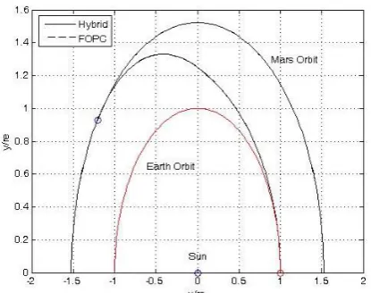
The optimal trajectories for hybrid and gradient methods are shown in Figure 2. The thrust angle histories obtained from Hybrid method and FOPC algorithm are compared and shown in Figure 3. This comparison was repeated for state histories in Figure 3. A good harmony can be seen from these figures. Both methods reach the same orbit at the same time and satisfy final constraints. Notice that the radial distance and velocities are in canonical units.

Fig 2: Comparison of optimal trajectories found by hybrid and gradient methods.

Fig 3: Comparison of Thrust Direction Angle Histories.

7.

CONCLUSIONS

A GA was used in conjunction with a gradient method (FOPC algorithm) to optimize an interplanetary trajectory. The reliance of the gradient method on earlier solutions and its sensitivity to the quality of the initial guesses were eliminated by relying on the GA to search the parameter space to find the location of the globally optimal solution. The FOPC algorithm was used to refine the parameter set found by the GA, improving the precision of the final answer beyond what would be possible by the use of the GA alone. To prove that the final solution obtained by hybrid method is a true global minimum, the result was compared against one obtained with the FOPC algorithm with assumption that a very good initial guess is available. Both methods reached the same orbit at the same time, satisfied final constraints, and had similar control and state histories. Hybrid method proposed is efficient and robust in achieving optimal solution when boundary conditions were treated as equality constraints.

8.

REFERENCES

9. Wuerl, A., Carin, T., Barden, E. 2003. Genetic Algorithm and Calculus of Variations-Based Trajectory Optimization Technique, Journal of Spacecraft and Rockets, V. 40, No. 6.

10. Dewell, L., Menon, P. 1999. Low-Thrust Orbit Transfer Optimization Using Genetic Search, AIAA Guidance, Navigation, and Control Conference and Exhibit, AIAA, Reston, USA.

11. Betts, J. T. 1998. Survey of Numerical Methods for Trajectory Optimization, Journal of Guidance, Control and Dynamics, Vol. 21, No. 2.

12. Beveridge, G. S., and Schechter, R. S. 1970. Optimization: Theory and Practice, New York, McGraw-Hill.

13. Bulirsch, R., Montrone, F., and Pesche, H. 1996. Abort Landing in the presence of a Windshear as a Minimax Optimal Control Problem, Part 2: multiple Shooting and Homotopy, Journal of Optimization Theory and Applications, Vol. 33, No. 6.

14. Reeves, C. R. 1996. Heuristic search methods: A review, In D. Johnson and F. O'Brien (1996) Operational Research: Keynote Papers, Operational Research Society, Birmingham, UK.

15. Gage, P.J., Braun, R.D., and Kroo, I.M. 1995. Interplanetary Trajectory Optimization Using a Genetic Algorithm, Journal of Astronautical Sciences, Vol. 43, No. 1.

16. Carter, M.T., and Vadali, S.R. 1995. Parameter Optimization Using Adaptive Bound Genetic Algorithms, American Astronomical Society, AAS Paper 95-140.

17. Pinon, E., III, and Fowler, W.T. 1995. Lunar Launch Trajectory Optimization Using a Genetic Algorithm, American Astronomical Society, AAS Paper 95-142.

18. Bryson, A., and Ho, Y. 1975. Applied Optimal Control, Revised Printing, Hemisphere, New York.

19. Aerospace Trajectory Optimization Using Direct Transcription and Collocation, http://www.cdeagle. cnchost.com/ommatlab/dto_matlab.pdf

20. Bryson, A.E. 1998. Dynamic Optimization, Prentice Hall.

21. Rauwolf, G.A, Coverstone-Carroll, V.L. 1996. Near-Optimal Low-Thrust Orbit Transfers Generated by a Genetic Algorithm, Journal of Spacecraft and Rockets, Vol. 33, No. 6.

22. Bate, R.R., Mueller, D.D., and White, J.E. 1975. Fundamentals of Astrodynamics, 1st ed., Dover, New York.

23. Ansari, N. 1997. Computational Intelligence for Optimization, Kluver Academic Publishers.

24. Holland, J. 1975. Adaptation in Natural and Artificial Systems, University of Michigan Press, Ann Arbor.

25. Goldberg, D.E. 1989. Genetic Algorithms in Search, Optimization, and Machine Learning, Addison-Wesley.

26. Hsiao J. Hui-wen, Literature Review–Genetic Algorithms,

http://www.homepages.inf.ed.ac.uk/s0231692/resume /GeneticAlgorithmNew.pdf.

27. Renders, J-M., and Flasse, S. P. 1996. Hybrid Methods Using Genetic Algorithms for Global Optimization, IEEE Transactions on Systems, Man, and Cybernetics-Part B: Cybernetics, Vol.26, No. 2, 243-258.

28. Carin, T. P., Bishop, R. H., Fowler, W. T., and Rock, K. 1998. Interplanetary Flyby Mission Optimization Using a Hybrid Global/Local Search Method, Journal of Spacecraft and Rockets, Vol. 37, No. 3.

29. Hartmann, J. W., Coverstone-Carroll, V. L., Williams, S. N. 1998. Optimal Interplanetary Spacecraft Trajectories via a Pareto Genetic Algorithm, Journal of Astronautical Sciences, Vol. 46, No. 3.

30. Hoffmeister F., Back T. 1991. Genetic algorithms and evolution strategies: similarities and differences, In: Schefel H. P., Manner R.(eds.) Parallel Problem Solving from Nature, Proceedings of 1st _Workshop, Dortmund, Germany.

31. Perhinschi, M. G. 1997. A Modified Genetic Algorithm for the Design of Autonomous Helicopter Control System, Proceedings of the AIAA Guidance, Navigation, and control Conference, New Orleans, LA, USA.