Taylor Series Prediction of Time Series Data with Error
Propagated by Artificial Neural Network
S. Alamelu Mangai
Research Scholar, Dept. of Computer Applications,
School of Information Technology,
Madurai Kamaraj University, Madurai-625021
India
B. Ravi Sankar
Scientist, MPAD/MDG ISRO Satellite Centre
Bangalore-560017 India
K. Alagarsamy,
Ph D Associate Professor, Dept. of Computer Applications,School of Information Technology,
Madurai Kamaraj University, Madurai-625021
India
ABSTRACT
Modeling and forecasting of a time series data is an integral part of the Data Mining. Sun spot numbers observed on the sun are a good candidate for a time series. A number of linear statistical models are discussed in this paper because Taylor series has similarity with an Auto Regressive model. A new algorithm based on Taylor series expansion and artificial neural network is presented. Based on Taylor series algorithm and ARIMA model, the Sunspot numbers are forecasted and compared.
General Terms
Time Series, modeling, forecasting, ARIMA model, Random process.
Keywords
ARIMA, Artificial Neural Network, Taylor series, Time Series.
1.
INTRODUCTION
It is important to predict the space weather to safe guard our satellites and power grids. Solar activity is the driver of space weather. Thus it is important to be able to predict the violent eruptions such as coronal mass ejections (CME) and solar flares. These solar activities are correlated to the sun spot numbers observed and the correlation involves a lot of physics which is beyond the scope of the manuscript. Thus the scope of the manuscript is limited to predict the sun spot numbers which is a good candidate for time series modeling.
The remainder of this research is organized as follows. Section 2 contains a literature review. In section 3, the theory behind some of the stationary stochastic models and an introduction to neural networks is presented. The reason for discussing linear regression model in section 3 is that the Taylor series resembles like an Auto Regressive series. Section 4 introduces the concept of Taylor series expansion for a discrete time signal. Based on the Taylor series algorithm, sun spot numbers are modeled and forecasted in section 5. Section 6 concludes this work.
2.
LITERATURE REVIEW
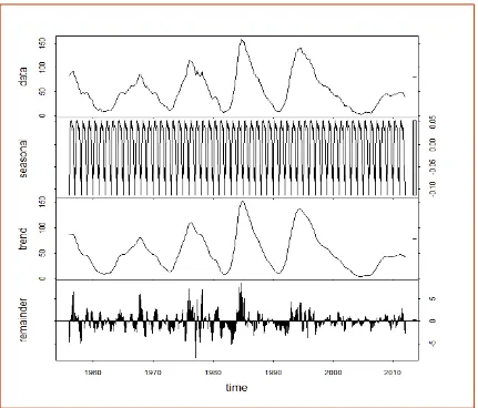
Time series data consists of four components: trend, seasonal effect, cyclical, and irregular effect. For the sun spot numbers these components are represented in figure.1. In a time series the future value is predicted from the past values assuming that the future value will be a slight perturbation of past values. This kind of prediction is called regression models. A brief review of linear regression models is presented in section 3.
Box and Jenkins [1] developed the autoregressive moving average to predict time series. The ARIMA model is used for prediction of non-stationary time series when linearity between variables is supposed. However, in many practical situations, linearity is not valid. For this reason, ARIMA models do not produce effective results when used for explaining and capturing nonlinear relations of many real world problems, which results in increased forecast error.
Artificial neural network (ANN) models are part of an important class that has attracted a considerable attention in many applications. Artificial Neural Networks are used to approximate non-linear functions. Peter Zhang [2] developed a hybrid ARIMA and Neural Network based model to forecast a time series.
―Qiang Yang et al.‖ [3] developed a Cache Replacement Policy based on Taylor series prediction. ―Marzi et al.‖ proposed a hybrid model based on Black-Scholes model and neural network for forecasting financial market [4]. The hybrid model outperformed the Black-Scholes model. A hybrid neural network algorithm which uses ant colony optimization algorithm for training the ANN is used to forecast the short term load in electricity [5]. Neural network based frequency analysis method was used to predict the rainfall in Indian geographical region [6]. Short term load forecasting of Power System based on different types of neural network was studied by ―Quaiyum et al.‖ [7].
Figure 1: Decomposition of the original signal into seasonal trend and remainder terms.
RMSE (Root Mean Square Error), respectively.Currently McNish-Lincoln technique is used to predict the sun spot number in NOAA/NASA [8].
3.
LINEAR STATISTICAL MODELS
AND OVERVIEW OF ANN
3.1
Linear Regression Models
In this section some of the linear statistical models for time series analysis are presented [9]. It is assumed that the time series values observed are the realizations of random variables
1
Y
, . . . ,Y
T which are in turn part of a larger stochastic process {Y
t :t
Z
}. It is this underlying process that will be the focus for the theoretical development. There are four different standard statistical models available namely AR(P), MA(q), ARMA(p,q) and ARIMA(p,d,q). There definitions are given below.3.1.1
Autoregressive Series
If
Y
tsatisfies the following equation t p t p tt
Y
Y
Y
1 1
...
(1)(Where
t is white-noise and
u are constants) thenY
t is called an autoregressive series of order p, denoted by AR(p). Autoregressive series are important because of the followingproperties.
They have a natural interpretation — the next value observed is a slight perturbation of a simple function of the most recent observations.
It is easy to estimate their parameters. It can be done with standard regression software.
They are easy to forecast. Again standard regression software will do the job.
3.1.2
Moving Average Series
A time series {
Y
t} which satisfies the following equation qt q t
t t
Y
1
1
...
(2)3.1.3
Auto Regressive Moving Average Series
If a time series satisfies the following equation
q t q t t p t p t
t
Y
Y
Y
1 1
...
1
1
...
(3)
(With {
t} white noise) then it is called an autoregressive-moving average series of order (p,q), or an ARMA(p,q)series. An ARMA(p,q) series is stationary [9] if the roots of the polynomial p pz
z
...
1
1 (4)lie outside the unit circle.
3.1.4
Auto Regressive Integrated Moving Average
Series
If
W
t
dY
t is an ARMA(p,q) series thenY
t is said to be an integrated autoregressive moving average(p,d,q) series, denoted by ARIMA(p,d,q). If one writes
pp
L
L
L
1
1
...
(5) and
qq
L
L
L
1
1
...
(6) then the operator formulation representation of ARIMA(p,d,q)is given below.
t
t dL
Y
L
(7)
3.2
System Identification
Here the task is to identify an appropriate model for the given observations. For this one needs to examine two functions namely autocorrelation function (acf) and partial auto correlation function (pacf). One has to first estimate the acf and pacf .
If the acf exhibits slow decay and the pacf cuts off sharply after lag p then the model would be AR(p).
If the pacf shows slow decay and the acf cuts off after lag q, then the appropriate model would be MA(q).
If both the acf and pacf show slow decay, then the appropriate model would be ARMA. In this case the orders are not clear and hence it is recommended to start with ARMA(1,1) and then move on to higher order [9].
3.3
Overview of Artificial Neural Network
Neural networks consist of a large class of different architectures. In many cases, the issue is approximating a static nonlinear, mapping f (x) with a neural network fNN(x),
where x∈RK. The most useful neural networks in function
approximation are Multi Layer Perceptron (MLP) and Radial Basis Function (RBF) networks. In this analysis, MLP network is employed. The following steps summarize the training method for a Multi-Layer Perceptron network.
The structure of the network is first defined. In the network, activation functions are chosen and the network parameters, weights and biases, are initialized.
The parameters associated with the training algorithm like error goal, maximum number of epochs (iterations), etc. is defined.
The training algorithm is called.
After the neural network has been determined, the result is first tested by simulating the output of the neural network with the measured input data. This is compared with the measured outputs.
Final validation must be carried out with independent data. The inherent problem with neural network is that they may get stuck in local minima.
4.
TAYLOR SERIES PREDICTION
4.1
Taylor Series
The Taylor series is named after the British mathematician Brook Taylor (1685-1731). Its definition was given like this [10]: If
f
has a power series representation (expansion) at point a and the radius of convergence of the power series is0
R
, that is, if
x
c
x
a
x
a
R
f
nn
n
,
0
(8)
then the coefficients are given by the formula
!
n
a
f
c
nn
(9)Therefore,
f
must be in the following form:
...
!
...
!
2
''
!
1
'
!
2 0
n n n n na
x
n
a
f
a
x
a
f
a
x
a
f
a
f
a
x
n
a
f
x
f
(10)The series in the above equation is called the Taylor series of the function
f
ata
and functionf
is called analytic ata
. From the above definition, it is clear thatf
(
x
)
is the limit of a sequence of partial sums. In the case of Taylor series, the partial sums are:
n
ni i n
a
x
n
a
f
a
f
a
x
a
f
a
f
a
x
i
a
f
x
T
!
...
!
2
'
'
!
1
'
!
(11) nT
is called nth-degree Taylor polynomial off
ata
. If we denoteR
nbe the remainder of the series, then
x
f
x
T
x
R
n
n (12)In a time series,
T
(
n
1
)
is given by the following formula.
...
!
2
''
!
1
'
1
T
n
T
n
T
n
n
T
Where
k k n T n T nT'
k
k
n
T
n
T
n
T
'
'
'
'
and so on.
In this analysis, the Taylor series consists of up to eight coefficients. The Taylor series used in this analysis is given below. ) 8 ( 5 92 . 9 ) 7 ( 3 38 . 1 ) 6 ( 0104 . 0 ) 5 ( 0555 . 0 ) 4 ( 2259 . 0 ) 3 ( 6795 . 0 ) 2 ( 3590 . 1 ) 1 ( 3591 . 1 ) ( 5 . 0 ) 1 ( n T e n T e n T n T n T n T n T n T n T n T (14)
5.
APPLYING TAYLOR SERIES TO
SUNSPOT NUMBERS
The Taylor series is linear and hence the residual part consists of non-linear terms. The residuals are used to train a neural network because neural networks are well suited to predict non-linear functions. The Taylor series is applied to the sun spot numbers for the period from 1956 to 2012. The Taylor series predicted value is subtracted from the original value to obtain the error or residual. This residual is used to train the artificial neural network.
The forecast is done in the following way. The Taylor series is used to predict the next value. This value is added with error propagated by the artificial neural network to arrive at the actual value.
An ARIMA model is fitted for the sun spot numbers with an order of (4,0,3)(0,0,2)(12). Where in the number (12) indicates the period of the sun spot number time series.
[image:4.595.56.272.462.569.2]Figure 2: Observed Sun spot numbers from 1956 to 2012.
[image:4.595.319.530.520.623.2]Figure 3: Taylor Series predicted Sunspot Numbers.
Figure 4: Original and Taylor series predicted.
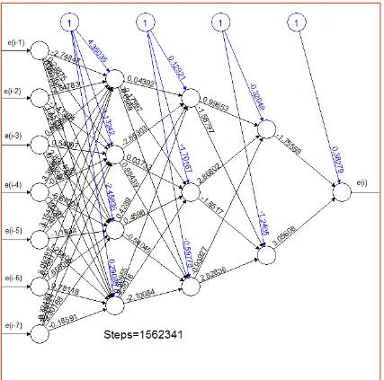
The observed sun spot numbers are plotted in figure.2. The Taylor series predicted are plotted in figure.3. Both observed and Taylor series predicted values are depicted in figure.4. The error residuals are plotted in figure.6. The schematic of the Artificial Neural Network used to propagate residuals is shown in figure.5. Figure.7 shows the error forecast using ANN. Figure.8 shows the forecast of Sunspot numbers using Taylor series algorithm and figure.9 shows the ARIMA fitted values.
Algorithm
1. Predict the next time series value using Taylor series prediction using eq. (14)
2. Obtain the residual between observed and Taylor series predicted.
3. Propagate the residual using Artificial Neural Network (ANN) whose schematic is shown in Figure.5. This ANN is already trained with the residuals.
4. For one step ahead forecasting, add the Taylor series predicted with residual that is propagated by Artificial Neural Network.
Figure 5: Schematic of the Artificial Neural Network used to propagate Residuals
[image:5.595.55.281.555.682.2]Figure 8: Sunspot number with Taylor series forecast and error propagated by ANN.
Figure 9: Sunspot number forecast with ARIMA model.
6.
CONCLUSION
Taylor series is a linear regression model and hence the artificial neural network provides the non-linear component of the algorithm. It can be used to predict a very few instants of future values and it is equivalent to other models. As the prediction time grows the ANN propagated error approaches zero and overall model error becomes unusually large. In this analysis, values are forecasted for five years. A comparison was done between Taylor series algorithm and the ARIMA model using the Bayesian Information Criterion, where Taylor series algorithm had a lower BIC and RMSE value and hence is a good fit for the given data. The BIC and RMSE values for both the models are given in table 1.
Table 1. The comparison of the models by RMSE and BIC
RMSE BIC
ARIMA 0.979 101.276
7.
REFERENCES
[1] Box G.E.P, Jenkins G.M and Reinsel G.C, 1994, ―Time Series Analysis, Forecasting and Control‖, Prentice Hall.
[2] G. Peter Zhang, “Time series forecasting using a hybrid ARIMA and neural network model‖, ELSEVIER, Neurocomputing 50 (2003) 159 – 175.
[3] Qiang Yang, Haining Henry Zhang and Hui Zhang, ―Taylor Series Prediction: A Cache Replacement Policy based on Second-order Trend Analysis‖, Hawaii International Conference on System Sciences 01/2001; 5:5023, ISBN 0-7695-0981-9.
[4] Hosein Marzi and Mark Turnbull, ―Use of Neural Networks in Forecasting Financial Market‖, 2007 IEEE International Conference on Granular Computing, IEEE Computer Society.
[5] Chengqun Yin, Lifeng Kang and Wei Sun, ―Hybrid Neural Network Model for Short-Term Load Forecasting‖, Third International Conference on Natural Computation (ICNC 2007), IEEE Computer Society.
[6] Seema Mahajan and Himanshu Mazumdar, ―Rainfall Prediction using Neural Net based Frequency Analysis Approach‖, International Journal of Computer Application, Volume 84 – No 9, December 2013.
[7] Salman Quaiyum, Yousuf Ibrahim Khan, Saidur Rahman and Parijat Barman, ―Artificial Neural Network based Short Term Load Forecasting of Power Systems‖, International Journal of Computer Application, Volume 30 – No 4, September 2011
[8] McNish.A.G and J.V.Lincoln, Transactions of American Geophysical Union 30 (1949) 673-685.
[9] RossIhaka,“Time Series Analysis‖, available at the URL https://www.stat.auckland.ac.nz/~ihaka/726/notes.pdf