http://dx.doi.org/10.4236/jbise.2014.76035
How to cite this paper: Boutayeb, W., et al. (2014) Mathematical Modelling and Simulation of β-Cell Mass, Insulin and Glucose Dynamics: Effect of Genetic Predisposition to Diabetes. J. Biomedical Science and Engineering, 7, 330-342. http://dx.doi.org/10.4236/jbise.2014.76035
Mathematical Modelling and Simulation of
β
-Cell Mass, Insulin and Glucose Dynamics:
Effect of Genetic Predisposition to Diabetes
Wiam Boutayeb1*, Mohamed E. N. Lamlili1, Abdesslam Boutayeb1, Mohamed Derouich2 1URAC04, LaMSD, Department of Mathematics and Computer Sciences, Faculty of Sciences,
University Mohammed First, Rabat, Morocco
2National School of Applied Sciences, University Mohammed First, Rabat, Morocco
Email: *[email protected]
Received 25 March 2014; revised 29 April 2014; accepted 6 May 2014
Copyright © 2014 by authors and Scientific Research Publishing Inc.
This work is licensed under the Creative Commons Attribution International License (CC BY).
http://creativecommons.org/licenses/by/4.0/
Abstract
Worldwide, diabetes is affecting 370 million people, causing nearly five million deaths and absor- bing more than 471 billion USD per year. Mathematical models have been developed to simulate, analyse and understand the dynamics of β-cells, insulin and glucose. In this paper, we consider the effect of genetic predisposition to diabetes on dynamics of β-cells, glucose and insulin. We assume that the β-cell dynamics is governed by the differential equation:
(
) ( )
( )
(
( )
( )
)
( )
2 d
= 1 1
d
β
β ε β t ε β
r t g hG t iG t t
t − − K + − + − . The model indicates different behaviours
according to the presence or absence of genetic predisposition. In presence of predisposition (ε = 1), the model shows three equilibrium points: a stable physiological equilibrium point (G = 100, I = 20, β = 600), a stable trivial pathological equilibrium point (G = 600, I = 0, β = 0) and a saddle point (G = 250, I = 9.8, β = 129.36). In absence of predisposition (ε = 0), the model has only two equili-brium points: an unstable pathological equiliequili-brium point (G = 600, I = 0, β = 0) and a stable physi-ological equilibrium point (G = 82.6, I = 23, β = 900). In order to see how physical activity, obesity and other factors affect insulin sensitivity, simulations are carried out with different values of in-sulin induced glucose uptake rate (c), β-cell maximum insulin secretory rate (d) and environmen-tal capacity (K).
Keywords
Type 2 Diabetes, Mathematical Modelling, Physiological Equilibrium, Pathological Equilibrium
*
1. Introduction
Once associated with economic development and considered as a disease of the rich, diabetes is now affecting countries worldwide, threatening particularly low and middle-income countries. According to the last Interna-tional Diabetes Federation (IDF) report, about 80% of the 371 million diabetics live in low- and middle-income countries; nearly five million deaths were due to diabetes; and more than 471 billion USD was spent on health-care for diabetes in 2012 [1]. Due to its chronic nature with severe complications, diabetes needs costly pro-longed treatment and care, affecting individuals and societies, and raising the equity problem between and with-in countries [2]. Although prevalence of diabetes is increasing all over the world, the Middle East and North Africa region has the highest comparative prevalence of diabetes (11%). Six of the top 10 countries with the highest prevalence of diabetes (in adults aged 20 to 79 years) are in this region: Kuwait (21.1%), Lebanon (20.2%), Qatar (20.2%), Saudi Arabia (20%), Bahrain (19.9%) and UAE (19.2%) [1] [3]. Consequently, the di-rect and indidi-rect socio-economic burden of diabetes is exponentially increasing in this region [4] [5].
During the last decades, a large number of mathematical models have been developed to simulate, analyse and understand the dynamics of glucose and insulin leading to diabetes. Bolie (1961) was among the pioneers in this field. He introduced a simple linear model, using ordinary differential equations in glucose and insulin [6]. The most frequently used model is the well known minimal model published in early eighties by Bergman et al. [7]. Variant and critical versions based on the minimal model were published by different authors, including De-rouich and Boutayeb (adding physical effort) [8], De Gaetano and Arino (using delayed differential equations) [9], Li et al. (proposing a generalised model) [10] and Roy and Parker (extending the minimal model with free fatty acids) [11]. Other authors dealt with the dynamics of β-cells and the mechanisms leading to diabetes. Topp et al. published an interesting model on pathways to diabetes by considering β-cell mass, insulin, and glucose ki- netics [12]. Hernandez et al. proposed an extension of the Topp model by adding the surface insulin receptor dy- namics [13]. Using a mathematical model similar to the model of Topp et al., De Gaetano and collaborators in-troduced the concept of pancreatic reserve [14]. Gallenberger et al. proposed a model on the dynamics of glu-cose and insulin concentration connected to the β-cell cycle [15]. More generally and for modelling details, the reader is referred to recent reviews that dealt explicitly with different models using differential equations, de-layed differential equations, integro-differential equations, stochastic differential equations, optimal control and other methods for glycaemic control, blood glucose monitoring and devices devoted to diabetic prevention [16]-[22]. In this paper, we propose a mathematical model stressing the effect of genetic predisposition to di-abetes on the dynamics of β-cells, insulin and glucose.
2. Materials and Methods
2.1. Predisposition to Type 2 Diabetes
Obesity is generally associated with insulin resistance and hence represents a major risk factor for the develop-ment of type 2 diabetes [23]-[25]. However, not all obese people develop diabetes. In some of them, the β-cells mount a compensatory response to counter insulin resistance and the magnitude of compensation is probably ge- netically determined [25]. More generally, in lean and obese people not predisposed to develop diabetes, nor- moglycaemia is preserved since β-cells are able to sustain an adequate compensation to insulin resistance. In contrast, in people genetically susceptible to diabetes, the compensatory response is insufficient and β-cell de-compensation ensues [23]. Following the discussion of Poitout and Robertson on glucolipotoxicity and their hypothesis on the progressive β-cell dysfunction in lean and obese phenotypes with genetic predisposition [23], we propose a mathematical model of β-cell mass, glucose and insulin, extending the model of Topp et al. by adding the effect of genetic predisposition to diabetes.
2.2. The Mathematical Model
The mathematical model proposed is the following:
( )
( ) ( )
( )
(
)
d
= ,
d 1
cI t G t G
a bG t
( ) ( )
( )
(
)
( )
2 2 d = , dd t G t
I
fI t
t e G t
β
−
+ (2)
(
) ( )
( )
(
( )
( )
2)
( )
d= 1 1 .
d
t
r t g hG t iG t t
t K
β
β ε β ε β
− − + − + −
(3)
Most of mathematical models for glucose dynamics assume that the concentration of glucose in the blood is determined by a differential equation of the form d =
( )
( ) ( )
d G
a bG t cI t G t
t − − [7]-[9] [11]-[13]. In other
words, the concentration of glucose increases by a rate a (glucose production by liver and kidneys) and de-creases by a rate bG t
( )
(independent of insulin) and a rate cI t G t( ) ( )
representing the glucose uptake due to insulin sensitivity c.However, as indicated by Li et al., the relation cI t G t
( ) ( )
assumes a mass-action law while this term may be replaced by a more general expression [10]. Consequently, we use the Michaelis function, assuming that in- sulin-dependent net glucose tissue uptake takes the form:( ) ( )
( )
1 cI t G tG t
α + where
1
α is the half saturation constant,
and c
a is the maximum capacity. We assume thus that the variation of glucose is governed by the differential
equation:
( )
( ) ( )
( )
d=
d 1
cI t G t G
a bG t
t − −αG t + .
For insulin dynamics, we keep the same expression used in the model of Topp, assuming that the net insulin secretion rate can be modelled as a sigmoidal function of glucose level while insulin clearance is of the form
( )
fI t . Using a Hill function of the form
( )
( )
(
)
2
2
G t e G t+
as a sigmoid function reaching half its maximum at
1 2
=
G e , the insulin dynamics takes the form:
( ) ( )
( )
(
)
( )
2 2 d = dd t G t
I
fI t
t e G t
β
−
+ where β is the mass of pancreatic β-cells (mg), and secretion of insulin is supposed uniform for all β-cells, at the same maximal rate
mU d
ml mg d
.
Finally, as stressed earlier, we assume that the β-cell dynamics depends on genetic predisposition to diabetes and is, consequently governed by the differential equation:
(
) ( )
( )
(
( )
( )
2)
( )
d= 1 1
d
t
r t g hG t iG t t
t K
β
β ε β ε β
− − + − + −
This equation indicates that when ε = 1 (predisposition to diabetes) we simply get the expression used in the model of Topp, when ε = 0 (no predisposition to diabetes) we get a logistic equation in β
( )
t and for ε between 0 and 1 we get different combinations according to the level of predisposition. In the first right-hand term,( )
1r d− is the growth rate of β-cells and K (mg) represents the carrying capacity while the second right-hand term is the second-degree polynomial in G t
( )
used by Topp, meaning that the β-cell mass decreases outside the polynomial zeros and increases between the zeros (when the polynomial has two real zeros).3. Results and Discussion
3.1. The Model Behaviour
Table 1. Parameters for an average healthy person [12] [26].
Param Value Units Biological Interpretation
a 864 mg
dl d⋅ glucose production rate by liver when G = 0
b 1.44 1
d− glucose clearance rate independent of insulin
c 0.72 ml
μU d⋅ insulin induced glucose uptake rate
d 43.2 μU
ml d mg⋅ ⋅ β-cell maximum insulin secretory rate
e 20,000
2 2
mg
dl gives inflection point of sigmoidal function
f 432 1
d− whole body insulin clearance rate
g 0.06 1
d− β-cell natural death rate
h 0.84e-3 dl
mg d⋅ determines β-cell glucose tolerance range
i 0.24e-5
2
2 dl
mg d determines β-cell glucose tolerance range
K 900 mg Environmental capacity
r 0.01 1
d− growth rate of β-cells
α 0.01 1
mg inverse of half saturation constant
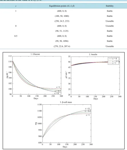
When ε = 0, our model has only two equilibrium points. A physiological equilibrium point (G = 82.6, I = 23, β = 900) and a trivial pathological equilibrium point (G = 600, I = 0, β = 0). For ε = 0.5, the model has three equi-librium points comparable to those obtained with ε = 1.
Stability analysis (see Appendix) shows that the physiological equilibrium point is stable for all values of ε. The pathological equilibrium point is stable when ε = 1 or 0.5 and more generally for values of ε different of 0 but it is unstable when ε = 0. The third equilibrium point is unstable when it exists (for values of ε different of 0) (Table 2).
3.2. Discussion
Assuming predisposition to diabetes (ε = 1), the qualitative behaviour of our model is similar to that of the mod-els developed by Topp et al. [12], Hernandez et al. [13], and De Gaetano et al. [14] represented by three equili-brium points: a stable physiological steady state (basal values of glycaemia and insulin); a trivial stable patho-logical severe diabetes steady state corresponding to a hyperglycaemic state with zero levels of β-cell mass and insulin, and an unstable saddle point with intermediate values of glycaemia, insulin and β-cell mass. Topp et al. and Hernandez et al. defined the bifurcation pathway to diabetes as a combination of parameters leading to the elimination of the physiological and saddle fixed points and making the pathological equilibrium point as a global attractor [12] [13]. De Gaetano et al. indicated that, when the saddle point exceeds a threshold, glucose toxicity prevails and β-cell mass eventually declines to zero, leading to the pathological steady state with zero insulin production [14]. The main difference of our model with respect to the previous models is the introduction of the effect of genetic predisposition to diabetes. Indeed, when ε = 0 (no predisposition to develop diabetes), our model gives only two equilibrium points: the trivial pathological point and the physiological steady state. Moreover, the pathological equilibrium point is unstable, leaving the physiological equilibrium point (with more realistic values for insulin (23) and β (900)) as the global attractor indicating that diabetes will not be developed.
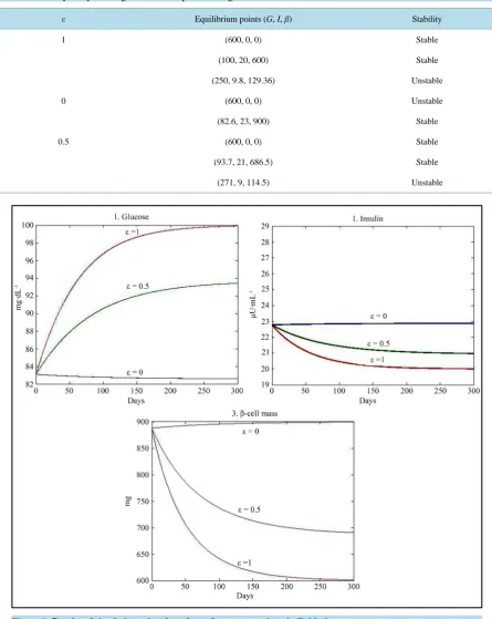
Table 2. Stability analysis using the values of parameters given in Table 1.
ε Equilibrium points (G, I, β) Stability
1 (600, 0, 0) Stable
(100, 20, 600) Stable
(250, 9.8, 129.36) Unstable
0 (600, 0, 0) Unstable
(82.6, 23, 900) Stable
0.5 (600, 0, 0) Stable
(93.7, 21, 686.5) Stable
(271, 9, 114.5) Unstable
Figure 1. Results of simulation using the values of parameters given in Table 1.
3.3. Simulation with Different Values of Parameters
In order to see how the parameter c in Equation (1) affects insulin sensitivity, a simulation was carried out with different values of c, d and K.
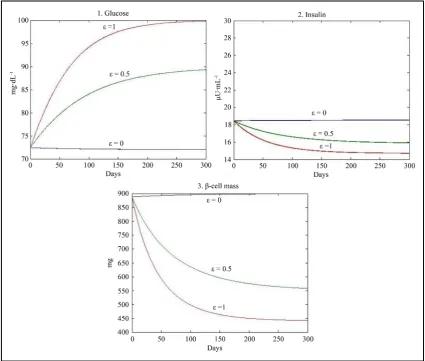
Taking into account the results of studies showing that physical exercise can increase insulin sensitivity by 36% [13], we used a simulation with the corresponding increased value of c (0.98) and obtained physiological equili-brium points (G = 100, I = 14.7, β = 441) with lower values of insulin and β-cell mass when ε = 1 and (G = 72, I = 18.5, β = 900) with a lower value of glucose when ε = 0 (Figure 2) (Table 3).
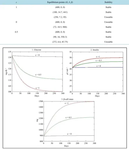
On the other hand, insulin resistance due to obesity and/or other factors has been shown to decrease insulin induced glucose uptake by 50% - 100% in both diabetic and non-diabetic subjects [12] [13]. In this direction, a simulation was used with a value of c decreased by 60% (c = 0.288), giving the physiological equilibrium point (G = 100, I = 50, β = 1500) with normoglycaemia associated with higher values of insulin and β-cell mass when ε = 1 and the equilibrium point (G = 130, I = 41.4, β = 900) when ε = 0 with values of insulin and β-cell mass lower than that of the case ε = 1 but with a value of glucose greater than normoglycaemia (Figure 3) (Table 4). At a first glance, the value of G = 130 when ε = 0 seems contradictory with the fact of no predisposition to di-abetes. However, the adaptation of β-cell suggests that, in this case, an increase of the β-cell mass (K) or the β-cell maximum insulin secretory rate (d) will assure near normoglycaemia as indicated by the following simu-lations:
[image:6.595.100.526.328.689.2]1) Following Rahier et al. who found that the β-cell mass increased with BMI in both diabetic (25%) and non- diabetic individuals (20%) [26], a third simulation was used with high level of insulin resistance and high carry-
Figure 2. Results of simulation using the values of parameters given in Table 1 with an increase in the value of c by
Table 3. Stability analysis using the values of parameters given in Table 1 with an increase in the value of c by 36%.
ε Equilibrium points (G, I, β) Stability
1 (600, 0, 0) Stable
(100, 14.7, 441) Stable
(250, 7.2, 95) Unstable
0 (600, 0, 0) Unstable
(72, 18.5, 900) Stable
0.5 (600, 0, 0) Stable
(90, 16, 550.3) Stable
(272, 6.6, 83.75) Unstable
Figure 3. Results of simulation using the values of parameters given in Table 1 with a decrease in the value of c by
60%.
ing capacity (K) giving the physiological equilibrium point (G = 100, I = 50, β = 1500) when ε = 1 and (G = 116, I = 45, β = 1125) when ε = 0 (Table 5).
Table 4. Stability analysis using the values of parameters given in Table 1 with a decrease in the value of c by 60%.
ε Equilibrium points (G, I, β) Stability
1 (600, 0, 0) Stable
(100, 50, 1500) Stable
(250, 24.5, 323.4) Unstable
0 (600, 0, 0) Unstable
(130, 41.43, 900) Stable
0.5 (600, 0, 0) Stable
(111, 46.5, 1224) Stable
[image:8.595.91.539.297.462.2](267, 23, 293) Unstable
Table 5. Stability analysis using the values of parameters given in Table 1 with an increase in the value of K by 25% and a
decrease in the value of c by 60%.
ε Equilibrium points (G, I, β) Stability
1 (600, 0, 0) Stable
(100, 50, 1500) Stable
(250, 24.5, 323.5) Unstable
0 (600, 0, 0) Unstable
(116, 45, 1125) Stable
0.5 (600, 0, 0) Stable
(105.6, 48, 1344) Stable
(268.35, 23, 291) Unstable
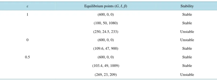
Table 6. Stability analysis using the values of parameters given in Table 1 with d = 60 and a decrease in the value of c by
60%.
ε Equilibrium points (G, I, β) Stability
1 (600, 0, 0) Stable
(100, 50, 1080) Stable
(250, 24.5, 233) Unstable
0 (600, 0, 0) Unstable
(109.6, 47, 900) Stable
0.5 (600, 0, 0) Stable
(103.4, 49, 1009) Stable
(269, 23, 209) Unstable
[image:8.595.89.536.494.659.2]Table 7. Stability analysis using the values of parameters given in Table 1 with d = 60, a decrease in the value of c by 60% and an increase in the value of K by 25%.
ε Equilibrium points (G, I, β) Stability
1 (600, 0, 0) Stable
(100, 50, 1080) Stable
(250, 24.5, 233) Unstable
0 (600, 0, 0) Unstable
(98, 51, 1125) Stable
0.5 (600, 0, 0) Stable
(99, 50, 1096) Stable
(270, 22.6, 207.4) Unstable
Figure 4. Results of simulation using the values of parameters given in Table 1 with a decrease in the value of c by
60%, an increase in the value of K by 25% and d = 60.
4. Conclusions
23, β = 900).
Assuming that physical exercise can increase insulin sensitivity by 36% whereas overweight/obesity and other factors may decrease insulin induced glucose uptake in both diabetic and non diabetic subjects, simulations were carried out with different values of the parameters c, d and K. The model shows that increased insulin sensitivity (higher value of c) due to physical exercise leads to a physiological equilibrium point with normoglycaemia and a low value of β-cell mass when ε = 1 and a value of glucose approaching normoglycaemia (G = 72) and a nor-mal value of β-cell mass when ε = 0. On the other hand, insulin resistance (lower value of c) can be compensated by an increased β-cell insulin secretory rate (d) or by an increased level of β-cell carrying capacity (K). In par-ticular, when both the values of K and d are increased, the model gives a physiological equilibrium point with nearly the same values of G, I and β for all values of ε. Consequently, our model stresses, as shown by experi-mental studies, the fact that not all people with insulin resistance develop diabetes. More interestingly, our mod-el confirms the idea that non diabetic and especially pre-diabetic people may avoid the evolution towards type 2 diabetes by acting on the risk factors, especially physical activity and overweight/obesity.
Author’s Contributions
The three authors participated equally to this paper. They read and approved the final manuscript.
Competing Interests
The authors declare that they have no competing interests.
References
[1] International Diabetes Federation (2012) IDF Diabetes Atlas. 5th Edition 2012 Update, Brussels.
http://www.idf.org/sites/default/files/IDF_Annual_Report_2012-EN-web.pdf
[2] Boutayeb, A. and Boutayeb, S. (2005) The Burden of Non Communicable Diseases in Developing Countries. Interna-tional Journal for Equity in Health, 4, 2. http://dx.doi.org/10.1186/1475-9276-4-2
[3] Boutayeb, A., Lamlili, M., Boutayeb, W., Maamri, A., Ziyyat, A. and Ramdani, N. (2012) The Rise of Diabetes Preva-lence in the Arab Region. Open Journal of Epidemiology, 2, 55-60. http://dx.doi.org/10.4236/ojepi.2012.22009
[4] Boutayeb, A., Boutayeb, W., Lamlili, M. and Boutayeb, S. (2014) Estimation of Direct Cost of Diabetes in the Arab Region. Mediterranean Journal of Nutrition and Metabolism, 7, 21-32.
[5] Boutayeb, W., Lamlili, M., Boutayeb, A. and Boutayeb, S. (2013) Estimation of Direct and Indirect Cost of Diabetes in Morocco. Journal of Biomedical Science and Engineering, 6, 732-738. http://dx.doi.org/10.4236/jbise.2013.67090
[6] Bolie, V.W. (1961) Coefficients of Normal Blood Glucose Regulation. Journal of Applied Physiology, 16, 783-788. [7] Bergman, R.N., Finegood, D.T. and Ader, M. (1985) Assessment of Insulin Sensitivity in Vivo. Endicrine Reviews, 6,
45-86. http://dx.doi.org/10.1210/edrv-6-1-45
[8] Derouich, M. and Boutayeb, A. (2002) The Effect of Physical Exercise on the Dynamics of Glucose and Insulin. Jour-nal of Biomechanics, 35, 911-917. http://dx.doi.org/10.1016/S0021-9290(02)00055-6
[9] De Gaetano, A. and Arino, O. (2000) Mathematical Modelling of the Intravenous Glucose Tolerance Test. Journal of Mathematical Biology, 40, 136-168. http://dx.doi.org/10.1007/s002850050007
[10] Li, J. and Kuang, Y. and Li, B. (2000) Analysis of IVGTT Glucose-Insulin Interaction Models with Time Delay. Dis-crete and Continuous Dynamical Systems Series B, 1, 103-124. http://dx.doi.org/10.3934/dcdsb.2001.1.103
[11] Roy, A. and Parker, R.S. (2006) Dynamic Modeling of Free Fatty Acids, Glucose, and Insulin: An Extended Minimal Model. Neurosiences, 8, 617-626.
[12] Topp, B. and Promislow, K. and De Vries, G. and Miura, R.M. and Finegood, D.T. (2000) A Model of β-Cell Mass, In- sulin, and Glucose Kinetics: Pathways to Diabetes. Journal of Theoretical Biology, 99A, 605-619.
http://dx.doi.org/10.1006/jtbi.2000.2150
[13] Hernandez, R.D., Lyles, D.J., Rubin, D.B., Voden, T.B. and Wirkus, S.A. (2001) A Model of β-Cell Mass, Insulin, Glucose and Receptor Dynamics with Applications to Diabetes. Technical Report, Biometric Department, MTBI Cor-nell University.
http://mtbi.asu.edu/research/archive/paper/model-%CE%B2-cell-mass-insulin-glucose-and-receptor-dynamics-applicat
ions-diabetes
E1479.
[15] Gallenberger, M., Castell, W.Z., Hense, B.A. and Kuttler, C. (2012) Dynamics of Glucose and Insulin Concentration Connected to the β-Cell Cycle: Model Development and Analysis. Theoretical Biology and Medical Modelling, 9, 46.
http://dx.doi.org/10.1186/1742-4682-9-46
[16] Bellazi, R., Nucci, G. and Cobelli, C. (2001) The Subcutaneous Rate to Insulin Dependent Diabetes Therapy. IEEE En- gineering in Medicine and Biology, 20, 54-64.
[17] Boutayeb, A. and Chetouani, A. (2006) A Critical Review of Mathematical Models and Data Used in Diabetology. Bio- Medical Engineering Online, 5, 43. http://dx.doi.org/10.1186/1475-925X-5-43
[18] Kansal, A.R. (2004) Modelling Approaches to Type 2 Diabetes. Diabetes Technology & Therapeutics, 6, 39-47.
http://dx.doi.org/10.1089/152091504322783396
[19] Landersdorfer, C.B. and Jusko, W.J. (2008) Pharmacokinetic/Pharmacodynamic Modelling in Diabetes Mellitus. Clini- cal Pharmacokinetics, 47, 417-448. http://dx.doi.org/10.2165/00003088-200847070-00001
[20] Makroglou, A., Li, J. and Kuang, Y. (2006) Mathematical Models and Software Tools for the Glucose-Insulin Regula-tory System and Diabetes: An Overview. Applied Numerical Mathematics, 56, 559-573.
http://dx.doi.org/10.1016/j.apnum.2005.04.023
[21] Parker, R.S., Doyle III, F.J. and Peppas, N.A. (2001) The Intravenous Route to Blood Glucose Control. IEEE Enginee- ring in Medicine and Biology, 20, 65-73. http://dx.doi.org/10.1109/51.897829
[22] Pattaranit, R. and van den Berg, H.A. (2008) Mathematical Models of Energy Homeostasis. Journal of the Royal Soci- ety Interface, 5, 1119-1135. http://dx.doi.org/10.1098/rsif.2008.0216
[23] Poitout, V. and Robertson, R.P. (2008) Fuel Excess and β-Cell Dysfunction. Endocrine Reviews, 29, 351-366.
http://dx.doi.org/10.1210/er.2007-0023
[24] Leonardi, O., Mints, G. and Hussain, M.A. (2003) β-Cell Apoptosis in the Pathogenesis of Human Type 2 Diabetes Mellitus. European Journal of Endocrinology, 149, 99-102. http://dx.doi.org/10.1530/eje.0.1490099
[25] Bagust and Beale, S. (2003) Deteriorating Beta-Cell Function in Type 2 Diabetes a Long-Term Model. Quarterly Jour- nal of Medicine, 96, 281-288. http://dx.doi.org/10.1093/qjmed/hcg040
[26] Rahier, J., Guiot, Y., Goebbels, R.M., Sempoux, C. and Henquin, J. (2008) Pancreatic Beta Cell Mass in European Subjects with Type 2 Diabetes. Diabetes, Obesity and Metabolism, 10, 32-42.
http://dx.doi.org/10.1111/j.1463-1326.2008.00969.x
Appendix
The equilibrium points satisfy the equations:
( )
( ) ( )
( )
(
)
d
= = 0
d 1
cI t G t G
a bG t
t − − αG t + (4)
( ) ( )
( )
(
)
( )
2 2 d= = 0
d
d t G t
I
fI t
t e G t
β
−
+ (5)
(
) ( )
( )
(
( )
( )
2)
( )
d= 1 1 = 0
d
t
r t g hG t iG t t
t K
β
β ε β ε β
− − + − + −
(6)
When ε = 1, we can easily compute the three equilibrium points of the system: P0:
(
G=a b= 60 0, = 0,I)
= 0β ; P1:
(
G I1, ,1 β1)
and P2:(
G I2, 2,β2)
.Where
(
)
1 22
1
4
= = 100
2
h h gi
G
i
− + −
−
(
1)(
1)
1
1
1
= a bG G = 20
I
cG α
− +
(
2)
1 1
1 2
1
= e G fI = 600 dG
β +
(
2)
1 2 24
= = 250
2
h h gi
G
i
− − −
−
(
2)(
2)
2
2
1
= a bG G = 9.8
I
cG α
− +
(
2)
2 2
2 2
2
= e G fI = 129.4 dG
β +
When ε≠1, the trivial equilibrium point is easily obtained P0:
(
G= 600, = 0,I β = 0)
, whereas the nontrivial equilibrium points are computed using numerical approximation by Maple: When ε = 0, P1:
(
G1= 82.6,I1= 23,β1= 900)
.When ε= 0.5, P1:
(
G1= 93.7,I1= 21,β1= 686.5)
and P2:(
G2 = 271,I2 = 9,β2 = 114.5)
.Stability Analysis
The Jacobian matrix of the system is given by:
(
) (
)
(
)
(
)
(
)
(
)
(
)
2 2 2 2 2 2 0 1 1 2 22 0 1 1
cI cG
b
G G
ed G dG
f
e G e G
h iG r g hG iG
K
α α
β
β
ε β ε ε
− − − + + − + + − − − + − + −
Consequently, stability analysis of the trivial equilibrium point is straightforward.
= f but the third eigenvalue (λ3 = r) is positive.
When ε = 1, P0: (G = 600, I = 0, β = 0) is stable since J P
( )
0 has three negative eigenvalues: λ1 = b, λ2 = −fand λ3=
(
− +g hG iG− 2)
.When ε = 1, P0: (G = 600, I = 0, β = 0) is stable since J P
( )
0 has three negative eigenvalues: λ1 = b, λ2 = −fand λ3 = 1
![Table 1. Parameters for an average healthy person [12] [26].](https://thumb-us.123doks.com/thumbv2/123dok_us/8044772.772368/4.595.91.528.103.403/table-parameters-average-healthy-person.webp)