https://doi.org/10.5194/hess-23-255-2019 © Author(s) 2019. This work is distributed under the Creative Commons Attribution 4.0 License.
An improved perspective in the spatial representation of soil
moisture: potential added value of SMOS disaggregated
1 km resolution “all weather” product
Samiro Khodayar1,2, Amparo Coll2, and Ernesto Lopez-Baeza2
1Institute of Meteorology and Climate Research (IMK-TRO), Karlsruhe Institute of Technology, Karlsruhe, Germany 2Earth Physics and Thermodynamics Department, University of Valencia, Valencia, Spain
Correspondence:Samiro Khodayar ([email protected]) Received: 18 January 2018 – Discussion started: 8 February 2018
Revised: 6 November 2018 – Accepted: 15 November 2018 – Published: 17 January 2019
Abstract. This study uses the synergy of multi-resolution soil moisture (SM) satellite estimates from the Soil Mois-ture Ocean Salinity (SMOS) mission, a dense network of ground-based SM measurements, and a soil–vegetation– atmosphere transfer (SVAT) model, SURFEX (externalized surface), module ISBA (interactions between soil, biosphere and atmosphere), to examine the benefits of the SMOS level 4 (SMOS-L4) version 3.0, or “all weather” high-resolution soil moisture disaggregated product (SMOS-L43.0;∼1 km). The added value compared to SMOS level 3 (SMOS-L3;
∼25 km) and SMOS level 2 (SMOS-L2;∼15 km) is inves-tigated. In situ SM observations over the Valencia anchor sta-tion (VAS; SMOS calibrasta-tion and validasta-tion – Cal/Val – site in Europe) are used for comparison. The SURFEX (ISBA) model is used to simulate point-scale surface SM (SSM) and, in combination with high-quality atmospheric information data, namely from the European Centre for Medium-Range Weather Forecasts (ECMWF) and the Système d’analyse fournissant des renseignements atmosphériques à la neige (SAFRAN) meteorological analysis system, to obtain a rep-resentative SSM mapping over the VAS. The sensitivity to realistic initialization with SMOS-L43.0 is assessed to sim-ulate the spatial and temporal distribution of SSM. Results demonstrate the following: (a) All SMOS products correctly capture the temporal patterns, but the spatial patterns are not accurately reproduced by the coarser resolutions, probably in relation to the contrast with point-scale in situ measurements. (b) The potential of the SMOS-L43.0product is pointed out to adequately characterize SM spatio-temporal variability, re-flecting patterns consistent with intensive point-scale SSM samples on a daily timescale. The restricted temporal
avail-ability of this product dictated by the revisit period of the SMOS satellite compromises the averaged SSM representa-tion for longer periods than a day. (c) A seasonal analysis points out improved consistency during December–January– February and September–October–November, in contrast to significantly worse correlations in March–April–May (in re-lation to the growing vegetation) and June–July–August (in relation to low SSM values < 0.1 m3m−3 and low spatial variability). (d) The combined use of the SURFEX (ISBA) SVAT model with the SAFRAN system, initialized with SMOS-L43.01 km disaggregated data, is proven to be a suit-able tool for producing regional SM maps with high accu-racy, which could be used as initial conditions for model sim-ulations, flood forecasting, crop monitoring and crop devel-opment strategies, among others.
1 Introduction
considered responsible for this (Western et al., 2002; Bosch et al., 2007; Rosenbum et al., 2012).
The response of soil moisture to precipitation changes largely depends on soil’s water capacity and climatic zones. Particularly, in dry climates such as the Iberian Peninsula (IP), soil moisture reacts quickly to changes in precipita-tion (Li and Rodell, 2013). Precipitaprecipita-tion variability and mean are positively correlated, thus, an increase in precipitation yields wetter soils, which in turn results in higher spatial vari-ability in soil moisture. An adequate representation of the high spatio-temporal variability in soil moisture is needed to improve climate and hydrological modelling (Koster et al., 2004; Brocca et al., 2010). Its impact has been seen on timescales from hours to years (e.g. ∼20 km scale – Tay-lor and Lebel, 1998; droughts – Schubert and Boche, 2004; decadal drying of the Sahel – Walker and Rowntree, 1977; hot extremes – and Hirschi et al., 2011; decadal simulations – Khodayar et al., 2015b). To obtain an appropriate repre-sentation of this variable, especially at high-resolution, is not an easy task, mainly because of its high variability. Methods for the estimation of soil moisture can be divided into three main categories, (i) measurement of soil moisture in the field, (ii) estimation via simulation models, and (iii) measurement using remote sensing. In general, in situ measurements are far from global (e.g. Robock et al., 2000), and model simu-lations present important biases. Therefore, we have to rely on space-borne sensors to provide such measurements, but until recent times no dedicated, long-term space mission for measuring moisture was attempted (Kerr, 2007).
Nowadays, by means of remote-sensing technology sur-face soil moisture is available at global scale (Wigneron et al., 2003). The best estimations result from microwave re-mote sensing at low frequencies (e.g. Kerr, 2007; Jones et al., 2011), and several global soil moisture products have been produced, such as those resulting from the European Space Agency’s Climate Change Initiative (ESA CCI, Liu et al., 2011), the Soil Moisture Active Passive satellite (SMAP; Entekhabi et al., 2010), the Advanced Microwave Scanning Radiometer-EOS (AMSR-E; Owe et al., 2008), the advanced scatterometer (ASCAT; Naeimi et al., 2009) and the Soil Moisture and Ocean Salinity (SMOS; Kerr et al., 2001) mis-sions.
The SMOS mission is the first space-borne passive L-band microwave (1.4 GHz) radiometer measuring soil mois-ture over continental surfaces, as well as ocean salinity, at low frequency (Kerr et al., 2001, 2010). SMOS delivers global surface soil moisture measurements (∼0–5 cm depth) at 06:00 LT and 18:00 LT in a revisit of less than 3 days at a spatial resolution of∼44 km. The benchmark of the mission is to reach accuracy better than 0.04 m3m−3for the provided global maps of soil moisture (Kerr et al., 2001).
SMOS data are not exempt from biases. Validating remote-sensing-derived soil moisture products is difficult, e.g. due to scale differences between the satellite footprints and the point measurements on the ground (Cosh et al., 2004).
How-ever, in previous years a huge effort has been made to val-idate the SMOS algorithm and its associated products. For this purpose, in situ measurements across a range of climate regions were used, assessing the reliability and accuracy of these products using independent measurements (Delwart et al., 2008; Juglea et al., 2010a; Bircher et al., 2012; Dente et al., 2012; Gherboudj et al., 2012; Sánchez et al., 2012; Wigneron et al., 2012). The strategy adapted by the European Space Agency (ESA) was to develop specific land product validation activities over well-equipped monitoring sites. An example of this is the Valencia anchor station (VAS; Lopez-Baeza et al., 2005) in eastern Spain, which was chosen as one of the two main test sites in Europe for the SMOS calibra-tion and validacalibra-tion (Cal/Val) activities. The validacalibra-tion sites were chosen to be slightly larger than the actual pixel (3dB footprint), thus, VAS covers a 50 km×50 km area. Within this area, a limited number of ground stations were installed, relying on spatialized soil moisture information using the SVAT (soil–vegetation–atmosphere transfer) SURFEX (ex-ternalized surface) model. Worldwide validation results re-veal a coefficient of determination (R2) of about 0.49 when comparing the∼5 cm in situ soil moisture averages with the SMOS level 2 (SMOS-L2) soil moisture (∼15 km). For ex-ample, validation results by Bircher et al. (2012) in west-ern Denmark show anR2of 0.49–0.67 (SMOS retrieved ini-tial soil moisture) and 0.97 (SMOS-retrieved iniini-tial temper-ature). Besides this, significant under- or overrepresentation of the network data (biases of – 0.092–0.057 m3m−3) is also found. Over the Maqu (China) and Twente (the Netherlands) regions, the validation analysis resulted in an R2 of 0.55 and 0.51, respectively, for the ascending pass observations, and of 0.24 and 0.41, respectively, for the descending pass observations. Furthermore, Dente et al. (2012) pointed out a systematic SMOS soil moisture (ascending pass observa-tions) dry bias of about 0.13 m3m−3for the Maqu region and 0.17 m3m−3for the Twente region. Validation of the SMOS level 3 (SMOS-L3) product (∼35 km) shows that the gen-eral dry bias in SMOS-L2 is also present in SMOS-L3 SM. This bias is markedly present in the ascending products and shorter time series as described in Sanchez et al. (2012) and Gonzalez-Zamora et al. (2015). In this case, the presence of dense vegetation is seen to increase root-mean-square error (RMSE) scores, whereas in low vegetated areas a lower dry bias is found (Louvet et al., 2015).
into 1 km soil moisture maps over the IP without significant degradation of the RMSE. This product has been evaluated using the REMEDHUS (REd de MEDición de la HUmedad del Suelo) soil moisture network in the semi-arid area of the Duero Basin, Zamora, Spain (Piles et al., 2014). Results show that downscaling maintains temporal correlation and root-mean-squared differences with ground-based measure-ments, hence capturing the soil moisture dynamics. Comple-mentary studies after Piles et al. (2011) have produced sim-ilar downscaled high-resolution SMOS level 4 (SMOS-L4) soil moisture products (e.g. Malbéteau et al., 2018; Djamai et al., 2016). Being similar, however, the algorithms creating them are totally different from those of SMOS-L4 products used in this study. Whereas SMOS-L4 products in this study proceed from the original SMOS-L2 (15 km resolution soil moisture) disaggregated by 1 km MODIS LST and the nor-malized difference vegetation index (NDVI), Malbéteau et al. (2018) and Djamai et al. (2016) products proceed from the original SMOS-L1 (15 km resolution brightness temper-ature).
A big limitation for the downscaling approach used in Piles et al. (2011) is the lack of information in cloudy con-ditions of the SMOS level 4 2.0 (hereafter named SMOS-L42.0), which significantly limits the availability and useful-ness of this product. In this study, we examine a new version of the SMOS-L4 product, the SMOS level 4 3.0 “all weather” disaggregated∼1 km SM (SMOS-L43.0), which was devel-oped and has been recently made available by SMOS-BEC (Barcelona Expert Center). In this advanced high-resolution soil moisture product, the limitation on clouds is modulated by the use of ERA-Interim LST data, thus providing soil moisture measurements independently of the cloud condi-tions.
Contrary to SMOS-L3 and SMOS-L2 products, which have been extensively validated as described above and used for assimilation purposes in models (e.g. De Lannoy et al., 2016), few studies deal with the disaggregated 1 km SMOS-L42.0and SMOS-L43.0products (mostly in relation to wild-fire activity), and validation efforts have only concentrated on the REMEDHUS soil moisture network in Zamora (north-western Spain; e.g. Piles et al., 2014). The objective of this paper is to provide information about the advantages and drawbacks and the added value of the disaggregated 1 km SMOS-L43.0 “all weather” soil moisture product with re-spect to coarser resolution products. The proposed investiga-tion covers a 1-year period (a complete hydrological cycle) and focuses on the semi-arid VAS area (eastern Spain) and the IP, where water availability and fire risk are big environ-mental issues, and knowledge of soil moisture conditions is thus of pivotal importance. Furthermore, as springtime soil moisture anomalies over the IP are believed to be a precursor to droughts and heat waves in Europe (Vautard et al., 2007; Zampieri et al., 2009), accurate monitoring and prediction of surface states in this region may be key for improvements in seasonal forecasting systems.
The following objectives are then pursued: (a) the exami-nation of soil moisture temporal and spatial distribution with SMOS-derived soil moisture products over the investigation domain using a multi-resolution approach for L3 (∼25 km), L2 (∼15 km) and L43.0(∼1 km), (b) validation with the in situ soil moisture measurements’ network (VAS) to estimate the reliability of the SMOS SM products, and (c) evaluation of the impact of realistic SM initialization using SMOS-L43.0 on point-scale and regional SURFEX (ISBA) model simula-tions over the VAS area.
This investigation is structured as follows. In Sect. 2, the study area and the data sets are presented, including the in situ network measurements, the SMOS data products, and the SURFEX (ISBA) model and related atmospheric forc-ings used. Section 3 summarizes the methodology applied. The results are discussed in Sect. 4. Finally, conclusions are drawn in Sect. 5.
2 Study area and data set
2.1 Investigation domain and in situ measurements over the VAS
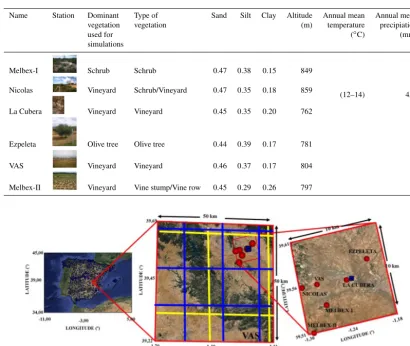
Me-Table 1.Characteristics of soil moisture stations within the VAS domain.
Name Station Dominant Type of Sand Silt Clay Altitude Annual mean Annual mean
vegetation vegetation (m) temperature precipiation
used for (◦C) (mm)
simulations
Melbex-I Schrub Schrub 0.47 0.38 0.15 849
(12–14) 451
Nicolas Vineyard Schrub/Vineyard 0.47 0.35 0.18 859
La Cubera Vineyard Vineyard 0.45 0.35 0.20 762
Ezpeleta Olive tree Olive tree 0.44 0.39 0.17 781
VAS Vineyard Vineyard 0.46 0.37 0.17 804
[image:4.612.92.502.78.424.2]Melbex-II Vineyard Vine stump/Vine row 0.45 0.29 0.26 797
Figure 1.Area of investigation and orography. Location of rain gauges from AEMET (Spanish State Meteorological Agency) is shown over the Iberian Peninsula (blue squares). The positions of the soil moisture network stations within the 10 km×10 km (OBS area) in the VAS (50 km×50 km) area are indicated by red circles.
teorología; Spanish State Meteorological Agency) network. Measurements are available for every 10 min.
2.2 The SMOS surface soil moisture products
ESA’s derived SMOS Soil Moisture level 2 (SMOS-L2) data product, ∼15 km, contains the retrieved soil moisture and optical thickness as well as complementary parameters such as atmospheric water vapour content, radio frequency in-terferences and other flags. The SMOS-L2 algorithms have been refined since the launch of SMOS, resulting in more precise SM retrievals (ARRAY, 2014). The SMOS-L3 prod-uct was obtained from the operational CATDS (Centre Aval de Traitement des Données) SMOS archive. This is a daily product that contains filtered data. The best estimation of SM is selected for each node when several multi-orbit re-trievals are available for a given day. A detection of partic-ular events is also performed in order to flag the data. The processing of the data separates morning and afternoon
or-bits. The aggregated products are generated from this funda-mental product. The SMOS-L4 2.0 data (SMOS-L42.0) with 1 km spatial resolution are provided by BEC and cover the IP, Balearic Islands, Portugal, southern France and northern Mo-rocco (34–45◦N and 10◦W–5◦E). A downscaling method
[image:4.612.93.502.87.344.2]down-scaling approach is based on Piles et al. (2014) and Sanchez-Ruiz et al. (2014), with the novelty of introducing ERA-Interim LST data in the MODIS LST and NDVI scape, thus providing soil moisture measurements independently of the cloud conditions. ERA-Interim provides a resolution of about 0.125◦, whereas MODIS is a∼1 km product. The evalua-tion of the SMOS-L4 2.0 and 3.0 products support the use of the “all weather” version, since it does not depend on cloud cover, and the accuracy of the estimates with respect to in situ data is improved or preserved (Piles et al., 2015; SMOS-BEC Team, 2016).
In this study, the SMOS-L2 V5.51 data coming from a L1C input product (obtained from MIRAS measurements), the SMOS-L3 V2.72 and the SMOS-L4 V3.0 are employed.
2.3 The SURFEX (ISBA) SVAT model
The SVAT model SURFEX (Le Moigne et al., 2009), module ISBA (Noilhan and Planton, 1989), is used to generate point-scale and spatially distributed SM at 1 km grid spacing and temporal fields from initial conditions and atmospheric forc-ing. SURFEX (ISBA) was developed at the National Cen-tre for Meteorological Research (CNRM) in Météo, France, and it has been widely validated over vegetated and bare sur-faces (e.g. Calvet et al., 1998). The ISBA scheme uses the Clapp and Hornberger (1978) soil water model and Darcy’s law for the estimation of the diffusion of water in the soil, and it allows for 12 land use and related vegetation parameteriza-tion types. Crops are considered for the VAS area, since the region is mainly composed of vineyards, almond and olive trees, and shrubs.
The surface characteristics are considered in the SVAT in-put, roughness and the fraction of vegetation are adopted from ECOCLIMAP (Masson et al., 2003), topography is ob-tained from GTOPO (GTOPO30 Documentation, 1996), and soil types are defined using FAO (FAO, 2014).
To obtain an accurate simulation of soil moisture in the study area, the model was originally calibrated by Juglea et al. (2010b) to be applied over the entire site for any season or year. Particularly relevant to this study is the specific defini-tion of the soil hydraulic parameters which they made for the VAS area, since most of the hydrological parameters are site dependent and are not available from SMOS observations. A new set of empirical equations as a function of the percent-ages of sand and clay was defined using Cosby et al. (1984) and Boone et al. (1999). New definitions and recommenda-tions by Juglea et al. (2010b) for the VAS area were adopted in this investigation.
Atmospheric forcing information: ECMWF and SAFRAN
High-quality atmospheric forcing is needed to carry out ac-curate simulations. To run the SURFEX (ISBA) model, the following atmospheric forcing data are needed: air
tempera-ture and humidity at screen level, atmospheric pressure, pre-cipitation, wind speed and direction, and solar and atmo-spheric radiation. Three different sets of atmoatmo-spheric forc-ing information are used in this study as input forcforc-ing for the SURFEX (ISBA) simulations: (a) SURFEX-OBS, which consists of meteorological data from three fully equipped sta-tions in the OBS area, MELBEX-I, MELBEX-II and VAS, (b) SURFEX-ECMWF, which consists of ECMWF (Euro-pean Centre for Medium-Range Weather Forecasts) data, and (c) SURFEX-SAFRAN, information from the SAFRAN (Système d’Analyse Fournissant des Renseignements At-mosphériques à la Neige) meteorological analysis system (Quintana-Seguí et al., 2008; Vidal et al., 2010).
Precipitation, air temperature, surface pressure, air-specific humidity, wind speed and direction, downward long-wave radiation, diffuse shortlong-wave radiation, downward di-rect shortwave radiation, snowfall rate and CO2
concentra-tion are used as input data from the aforemenconcentra-tioned me-teorological stations in the OBS area. A temporal resolu-tion of 10 min is available. From ECMWF, the dew point and temperature at 2 m, pressure, precipitation, and wind components are used as forcing data, with a 6 h temporal resolution and 0.125◦×0.125◦spatial resolution. Precipita-tion, air temperature, surface pressure, air specific humid-ity, wind speed, and downward shortwave and longwave ra-diation from SAFRAN are used as input information, with a spatial resolution of 8 km×8 km and an hourly tempo-ral resolution. In the last case, we have an optimal spatial and temporal distribution of the atmospheric forcing over the VAS area (∼50 km×50 km) and a rarely found complete database to force the land surface model. More details about the SAFRAN system and its validation in north-eastern Spain can be found in Quintana-Seguí et al. (2016).
3 Analysis methodology
In order to investigate the characteristics and potential added values of fine-scale SMOS-derived soil moisture, the spatial variability, the temporal evolution and the probability distri-bution are investigated. For this purpose, SMOS-derived soil moisture products at different spatial resolutions, in situ mea-surements and model simulations are jointly evaluated.
Hy-drological Cycle in the Mediterranean Experiment (HyMeX; Dobrinski et al., 2014) took place in the western Mediter-ranean, with the IP and particularly the Valencia region as tar-get areas. During the SON period of 2012, the special obser-vation period (SOP1; Ducrocq et al., 2014) took place with intensive experimental deployment over the area. This pro-vides us with valuable information about the environmental conditions as well as the occurrence of precipitation events in the investigation area. Particularly, precipitation in the IP during the autumn (SON) period of 2012 was above aver-age (Khodayar et al., 2016). It was also the hydrological season in which higher variability in the soil moisture was observed as a result of the precipitation distribution. Two unique events, one at the end of September (27–29) affect-ing southern and eastern Spain and the other at the end of November (19–20) affecting the Ebro Valley (Jansà et al., 2014), largely determined the positive anomaly in precipita-tion and soil moisture in this period.
SMOS-L3 (∼25 km), SMOS-L2 (∼15 km), and SMOS-L43.0 (∼1 km) are used for the evaluation of soil mois-ture distribution at different grid spacing. Piles et al. (2014) pointed out that differences may exist between SMOS-L3 and SMOS-L2 and the 1 km disaggregated soil moisture SMOS-L4 because of the distinct methodology used to ob-tain these products. Only SMOS descending passes or a mean between ascending and descending passes are used to calcu-late mean daily values of SMOS-derived soil moisture. Soil moisture derived from the afternoon orbits was found to be more accurate than the morning passes (Piles et al., 2014). The fine temporal resolution of the model simulations (1 h) and the observations (10 min) allow comparisons at the time of the SMOS overpasses. Because of the 3-day revisit pe-riod of the SMOS swath, the IP is not fully covered by the satellite on daily basis. However, despite identified difficul-ties (radio frequency interferences, missing data, etc.), the IP is well observed, with 1.5 days being the average observa-tion frequency over the IP. Only those images with coverage higher than 50 % are considered in our calculations. A con-servative remapping to coarser resolutions is applied, when required, to make comparisons among each other or with re-spect to ground-based observations on equal terms. Remap-ping allows point-to-point comparisons between these data sets. In addition to the yearly and seasonal approach, an ex-emplary short time period, 19 to 20 October 2012, is con-sidered. This corresponds to one of the periods in which an extreme precipitation event occurred in the Ebro Valley (at the end of November; Jansà et al., 2014). Therefore, high variability in the soil moisture distribution is expected.
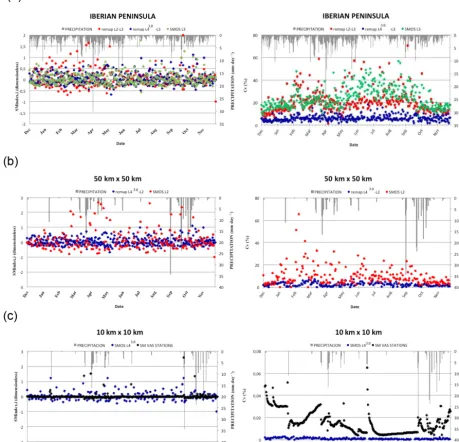
The coefficient of variation (CV), defined as the ratio of the standard deviation to the mean, of the precipitation and soil moisture fields over the IP, the VAS (50 km×50 km) and the OBS (10 km×10 km) areas are examined for the analysis of the spatial variability and its evolution in time. The soil moisture daily index (SMindex,i) is calculated to assess the evolution pattern, allowing the study of daily variations.
SMindex,i=(SMi+1-SMi)/ SMi, where SMi+1is the soil
moisture of the dayi+1, and SMiis the soil moisture of the day beforei.
For these calculations, SMOS afternoon (descending; Piles et al., 2014) orbits as well as observations at the time of the SMOS overpasses are selected. For the IP and VAS, SMOS-L2 and SMOS–L43.0 have been remapped to the coarser grid spacing for an adequate comparison. Ground-based observations are aggregated using a mean over all sta-tions for comparison with the corresponding SMOS-L43.0 data (the closest grid point is selected).
The reliability of SMOS-L3, SMOS-L2 and SMOS-L43.0 soil moisture products is evaluated by comparison with in situ soil moisture measurements in the OBS area. The spatial and temporal variability are considered as well as the prob-ability distribution. Different approaches are applied: (a) the nearest grid point is selected for point-like comparisons be-tween SMOS-L2 and SMOS-L43.0against in situ soil
mois-ture stations, to reduce sampling biases in this region of diverse soil characteristics (Table 1), and (b) SMOS-L43.0 soil moisture grid cells are averaged over the 10 km×10 km area and compared to the mean from the soil moisture net-work stations to address the issue related to spatial averag-ing due to the high spatial and temporal variability in the uppermost SSM. For the comparison between the SMOS-L2 and the in situ observations, when single ground-based stations are considered, the closest SMOS pixel is selected, and in the case of considering the OBS (10 km×10 km) or VAS (50 km×50 km) areas, the mean over all pixels whose centre falls within the area is used. For the comparison with SMOS descending passes the corresponding values from in situ measurements are considered. Additionally, a separation between wet days (precipitation over 1 mm d−1) and dry days
is applied to consider possible implications of wet and dry soils for SMOS measurements.
Linear regression, the coefficient of determination (R2), the mean bias (MB) and the root-mean-square deviation (RMSD) are used to predefine the accuracy. A de-biased or centred RMSD (CRMSD) is applied to discriminate the sys-tematic and random error components, removing the overall bias before calculating the RMSD.
sim-ulating the upper-level soil moisture variability of different soil characteristics (Table 1).
To try to simulate the spatial and temporal heterogeneity of the soil moisture fields over the VAS surface, the SURFEX (ISBA) scheme is used in combination with high-quality forcing data from ECMWF (hereafter SURFEX-ECMWF) and the SAFRAN system (hereafter SURFEX-SAFRAN) for spatialization purposes. Soil moisture initialization in spatial-ized SURFEX (ISBA) simulations requires a single represen-tative value for the whole simulation area. The benefit of ini-tializing the simulations with SMOS-L43.0data in compari-son to climatological means is discussed. In-situ soil mois-ture observations over the VAS area are considered for ver-ification. A comparison between SURFEX-SAFRAN point-scale and 10 km×10 km mean simulations initialized with SMOS-L43.0data is made against ground measurements to assess the accuracy of the simulated SSM maps.
4 Results
4.1 SMOS-derived soil moisture at different resolutions 4.1.1 Spatial variability on seasonal and sub-seasonal
timescales
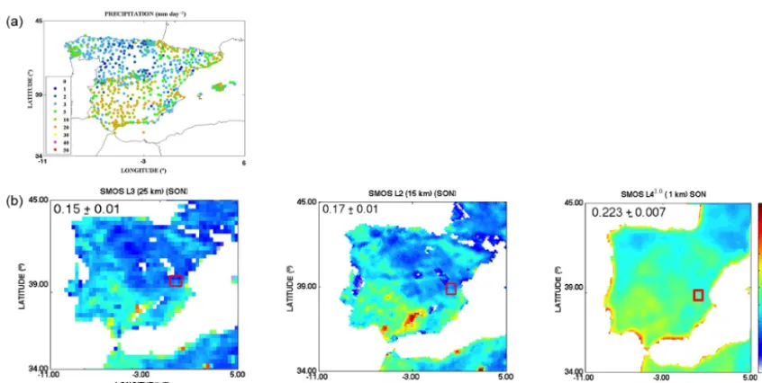
Figure 2a shows the north–south precipitation gradient for the SON period mean. The SSM satisfactorily reflects this gradient (Fig. 2b), but it does this more markedly for the L3 and L2 than the higher-resolution SMOS-L43.0, showing lower standard deviation in SMOS-L3 (∼
0.15±0.01), SMOS-L2 (∼0.17±0.01) and SMOS-L4 (∼
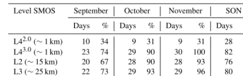
[image:7.612.308.548.96.171.2]0.22±0.007). The same performance is seen over the VAS domain (not shown). The SSM variability associated with the extreme precipitation events in this period is not well rep-resented in the SMOS-L43.0 seasonal mean. Table 2 shows the number of days (percentage) in which there is more than 50 % of data for the IP for each SMOS product. These pe-riods have been used as basis for the calculation of the spa-tial distributions in Fig. 2b. SMOS-L3 (88 %) and SMOS-L2 (84 %) show good coverage and a similar number of days. However, a large difference is observed with respect to the SMOS-L42.0product with only 28 days (32 %) of adequate coverage for the period of SON 2012. This is due to the prob-lem associated to the downscaling approach used to obtain the 1 km soil moisture maps, in which the lack of LST in-formation from MODIS VIS/IR satellite data in cloudy con-ditions (Sect. 2.2) constrains derived-SSM information. The availability and usefulness of this product is therefore signif-icantly reduced. The new product L43.0used in this study, in which the previous limitation is resolved using ERA-Interim-derived LST information, shows a coverage percentage of the order of 92 %, even higher than the SMOS-L3 and SMOS-L2 products. However, Fig. 2b demonstrates that the spatial rep-resentation of the seasonal mean does not improve with this
Table 2.Number of days (percentage) in which the SMOS (ascend-ing and descend(ascend-ing swaths) coverage is higher than 50 %.
Level SMOS September October November SON
Days % Days % Days % Days %
L42.0(∼1 km) 10 34 9 31 9 31 28 32
L43.0(∼1 km) 23 74 29 90 30 100 82 92
L2 (∼15 km) 20 67 28 90 28 93 76 83
L3 (∼25 km) 22 73 29 93 29 96 80 88
product, as a consequence of the limited temporal availabil-ity of the SMOS-derived SSM product dictated by the revisit period of the satellite.
In Fig. 3, only common available days from all differ-ent operational levels are selected for an inter-SMOS prod-uct comparison. When remapped to the same resolution (coarser grid spacing), comparable values are identified be-tween SMOS-L3, SMOS-L2 and SMOS-L43.0 for the JJA
and SON period, whereas relevant differences are pointed out from December to May. In this last period, we identify higher means for the SMOS-L43.0product and SMOS-L3 with re-spect to SMOS-L2, which is in agreement with a system-atic dry bias also identified for SMOS-L2 in previous studies (Sect. 1).
At sub-seasonal scales, e.g. event scale on the 19– 20 November 2012 (Fig. 4), the SMOS-L43.0product shows SSM mean and variability in the same range as the SMOS-L2 and SMOS-L3 products, but with a finer improved resolution representation of the spatial distribution. Comparisons with the mean ground-based SSM at the VAS (OBS area: 0.25±
0.0002) show better agreement with the mean SSM from the SMOS-L43.01 km disaggregated product (0.23±0.002) and poorer correlation with SMOS-L2 (0.20±0.002). The prob-lem of SMOS-L43.0on seasonal timescales vanishes at sub-seasonal (event) scales where the potential added value of the 1 km product is manifest.
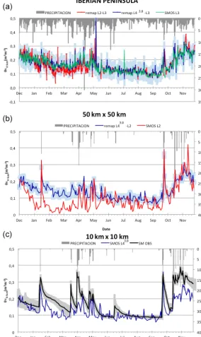
4.1.2 Temporal evolution of surface soil moisture data sets
differ-Figure 2. (a)spatial distribution of precipitation over the Iberian Peninsula from the network of rain gauges of AEMET. The period of September to November (SON) 2012 is shown.(b)spatial distribution of SMOS-derived soil moisture over the Iberian Peninsula (merged product: ascending and descending orbits, days with areal coverage higher than 50 % are considered).
Figure 3.SMOS-derived SSM product comparison from different operational levels over the Iberian Peninsula.
ences within in situ observations, SMOS responds well to soil moisture variations over time.
Although absolute values are not totally captured, all three SMOS products adequately reproduce the temporal dynam-ics at a regional scale. The systematic dry bias present in SMOS-L2 data (Piles et al., 2014) is evident, particularly in the first half of the year. A mean bias of the order of−0.09 to−0.07 m3m−3is identified for the DJF–MAM period; this difference is reduced to−0.02 m3m−3for the JJA–SON
pe-riod (Table 3). During the DJF–MAM pepe-riod the vineyards are bare, and only the vine stocks are present. The water con-tent of the vine stocks negatively impacts the SMOS mea-surements (Schwank et al., 2012).
Good agreement is found between the SMOS-L43.0 prod-uct and the mean of the in situ observations (the network’s variability (Fig. 6c; shaded grey contains the SMOS-L43.0 data). Scores confirm this result, particularly for the
peri-ods DJF and SON (slope∼1,R2∼0.7). Poorer correlation is found for the MAM (slope∼0.6, R2∼0.4). In this pe-riod, immediately after the precipitation events, soil mois-ture maxima are not always well capmois-tured by the SMOS-L43.0data, additionally showing a drying after this that is too rapid. This observation agrees with the SMOS mission’s in-ability of correctly measuring in situations when liquid water is present at the soil. The measured signal is perturbed dur-ing the vegetation growdur-ing season, which could explain the worse statistics. On the other hand, during JJA, a low slope of∼0.1 andR2of ∼0.01 could be in relation to SSM val-ues close to or lower than 0.1 m3m−3with very low spatial variability, which was found to be necessary for an adequate performance of the algorithm used for the derivation of the SMOS-L4 1 km product in Molero et al. (2016).
4.2 Spatial comparison at high-resolution: SMOS-L43.0versus ground measurements
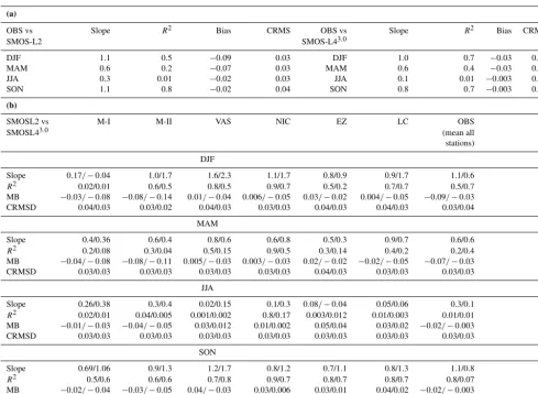
[image:8.612.49.286.340.458.2]Table 3.Statistics of the comparisons between SMOS-L2 and SMOS-L43.0soil moisture and ground-based measurements in the VAS network (the area covering the ground-based network has been called OBS; Fig. 1). SMOS descending orbits are selected for the comparison. Characteristics of the individual stations are given in Table 1. The acronyms for the names of the stations are as follows. M-I: Melbex-I, M-II: Melbex-II, VAS: VAS, NIC: Nicolas, EZ: Ezpeleta, LC: La Cubera. The period December 2011 to December 2012 is evaluated. The seasonal analysis follows the hydrological cycle. OBS stands for the average of (i) SMOS-L2 and/or SMOS-L43.0soil moisture values within the 10x10 km2where the ground-based network is placed, and (ii) in the case of the in situ observations, it refers to the mean of all stations.
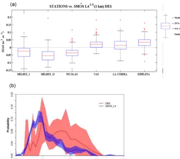
(a)shows a seasonal comparison between the mean of all in situ stations and the corresponding mean of SMOS-L2 and/or SMOS-L43.0 soil moisture values within the 10 km×10 km area. In(b)SMOS-L2 and SMOS-L43.0soil moisture observations are compared to point-like ground measurements using the closest grid point. The column on the right shows the mean of all stations.
(a)
OBS vs Slope R2 Bias CRMS OBS vs Slope R2 Bias CRMS
SMOS-L2 SMOS-L43.0
DJF 1.1 0.5 −0.09 0.03 DJF 1.0 0.7 −0.03 0.04
MAM 0.6 0.2 −0.07 0.03 MAM 0.6 0.4 −0.03 0.03
JJA 0.3 0.01 −0.02 0.03 JJA 0.1 0.01 −0.003 0.03
SON 1.1 0.8 −0.02 0.04 SON 0.8 0.7 −0.003 0.04
(b)
SMOSL2 vs M-I M-II VAS NIC EZ LC OBS
SMOSL43.0 (mean all
stations) DJF
Slope 0.17/−0.04 1.0/1.7 1.6/2.3 1.1/1.7 0.8/0.9 0.9/1.7 1.1/0.6
R2 0.02/0.01 0.6/0.5 0.8/0.5 0.9/0.7 0.5/0.2 0.7/0.7 0.5/0.7
MB −0.03/−0.08 −0.08/−0.14 0.01/−0.04 0.006/−0.05 0.03/−0.02 0.004/−0.05 −0.09/−0.03
CRMSD 0.04/0.03 0.03/0.02 0.04/0.03 0.03/0.03 0.04/0.03 0.04/0.03 0.03/0.04
MAM
Slope 0.4/0.36 0.6/0.4 0.8/0.6 0.6/0.8 0.5/0.3 0.9/0.7 0.6/0.6
R2 0.2/0.08 0.3/0.04 0.5/0.15 0.9/0.5 0.3/0.14 0.4/0.2 0.2/0.4
MB −0.04/−0.08 −0.08/−0.11 0.005/−0.03 0.003/−0.03 0.02/−0.02 −0.02/−0.05 −0.07/−0.03
CRMSD 0.03/0.03 0.03/0.03 0.03/0.03 0.03/0.03 0.04/0.03 0.03/0.03 0.03/0.03
JJA
Slope 0.26/0.38 0.3/0.4 0.02/0.15 0.1/0.3 0.08/−0.04 0.05/0.06 0.3/0.1 R2 0.02/0.01 0.04/0.005 0.001/0.002 0.8/0.17 0.003/0.012 0.01/0.003 0.01/0.01 MB −0.01/−0.03 −0.04/−0.05 0.03/0.012 0.01/0.002 0.05/0.04 0.03/0.02 −0.02/−0.003
CRMSD 0.03/0.03 0.03/0.03 0.03/0.03 0.03/0.03 0.03/0.03 0.03/0.03 0.03/0.03
SON
Slope 0.69/1.06 0.9/1.3 1.2/1.7 0.8/1.2 0.7/1.1 0.8/1.3 1.1/0.8
R2 0.5/0.6 0.6/0.6 0.7/0.8 0.9/0.7 0.8/0.7 0.8/0.7 0.8/0.07
MB −0.02/−0.04 −0.03/−0.05 0.04/−0.03 0.03/0.006 0.03/0.01 0.04/0.02 −0.02/−0.003
CRMSD 0.04/0.04 0.04/0.04 0.04/0.04 0.04/0.04 0.04/0.04 0.04/0.04 0.04/0.04
agreement between remotely sensed and in situ soil mois-ture measurements from the OBS network using the seasonal classification. To consider any uncertainties arising from spa-tial averaging, ground measurements are compared to point-like and 10 km×10 km SSM means. The 10 km×10 km area used covers the OBS area, i.e. the network of in situ mea-surements within the VAS. For comparison, all grid points from SMOS-L43.0 and SMOS-L2 included within the area are considered.
In Fig. 7a, the separation between days with and without precipitation (< 1 mm d−1) points out more similar correla-tions during dry days than wet days (RMSD∼0.015,R2∼
0.7) for SMOS-L43.0, whereas a slightly better agreement is
found for the dry days (not shown) for SMOS-L2. A system-atic mean dry bias of about 0.05 (dry days) to 0.08 (wet days) m3m−3is assessed for SMOS-L2, while a lower bias with changing sign is identified for the L43.0product (∼0.005 for
Figure 4.Spatial distribution of SMOS-derived soil moisture (merged product: ascending and descending orbits are considered) over the Iberian Peninsula (left) and the VAS (right) as a mean for the 19–20 November 2012(a)SMOS-L3 (∼25 km),(b)SMOS-L2 (∼15 km) and
(c)SMOS-L43.0(∼1 km). Empty pixels in(a)and(b)are indicative of a lack of data. Please be aware of the different colour scale used for the IP and VAS.
spatial patterns are captured at 1km with RMSD∼0.007 to 0.1 m3m−3, but in most cases, accuracy for the SMOS-L43.0 1 km disaggregated product is within the required range of less than 0.04 m3m−3(not shown). Higher RMSD is found
for SMOS-L2,∼0.008 to 0.13 m3m−3, accounting for the previously identified dry bias (∼(−0.14)–(−0.02)) reduced in SMOS-L43.0(∼(−0.08)–(−0.01)). The CRMSD is, in all cases,≤0.04 m3m−3. For all stations, better correlations are found in DJF and SON and poorer scores in JJA and MAM,
cor-Figure 5.Averaged SMOS products and averaged ground-based observations of soil moisture evolution over the Iberian Peninsula (IP;a), the VAS area(b)and the OBS area(c). Descending orbits are used. Precipitation from AEMET rain gauges are shown at the top of each plot. The soil moisture daily index (Ovindex,i; dimensionless) is shown in the left-hand plots, and the coefficient of variation (Cv, %) is shown in the right-hand plots.
relations. Worse statistics are found for Melbex-I, Melbex-II and Ezpeleta, probably in relation to the location of the soil moisture probes in rockier and orographically more complex areas, which are also in proximity to forest and man-made construction areas.
The soil moisture probability distribution function (PDF; Fig. 8b) of all in situ measurements versus SMOS-L43.0data reveals that the latter overestimates SSM below 0.1 m3m−3, values mainly observed during the JJA period. But an under-estimation occurs in the range between 0.1 and 0.3 m3m−3,
[image:11.612.69.528.78.519.2]Figure 6.Temporal evolution of surface soil moisture time series averaged over the Iberian Peninsula(a), the VAS area (50 km×50 km;b) and the OBS area (10 km×10 km;c). SMOS afternoon orbits are considered. Daily mean precipitation from the AEMET stations is shown on the top of each plot. SMOS and remapped SMOS products are indicated in the plots. Shaded areas show standard deviations.
4.3 SURFEX model simulations and realistic initialization with 1 km soil moisture data 4.3.1 SURFEX model simulations of selected stations
and realistic initialization
As a first step, the performance of the SURFEX (ISBA) SVAT model is evaluated. SURFEX (ISBA) point-like simu-lations are performed for all in situ soil moisture stations at
the VAS area to assess the usefulness of the model for further investigation (Table 4).
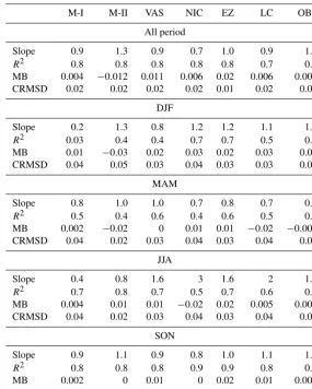
SURFEX (ISBA) simulations show good agreement with soil moisture ground-based observations at all stations, ad-equately capturing the associated spatio-temporal variability (slope∼1,R2∼0.7 to 0.9; MB∼0.1 m3m−3; CRMSD∼
Figure 7.Results of the seasonal analysis for the hydrological year starting in December 2011. Scatter plots of(a)SMOS-L43.0SSM (as-cending and des(as-cending orbits) versus averaged 10 km×10 km in situ soil moisture measurements for days with precipitation (left) and for days without precipitation (right; < 1 mm d−1).(b)SMOS-L2 and SMOS-L43.0SSM (descending orbits) versus averaged 10 km×10 km in situ soil moisture measurements.(c)SMOS-L2 and SMOS-L43.0SSM (descending orbits) versus point-like ground measurements from MELBEX-I station, using the closest grid point. Segments are linear fit of seasonal data (3 months of data). Statistics for individual compar-isons at all stations are summarized in Table 3.
in the SON period (R2∼0.9 for all stations), but CRMSD is
≤0.04 m3m−3for all stations at all periods.
Using the mean of the ground-based measurement on the day of the model simulation initialization (realistic initializa-tion; REAL-I) the temporal mean comparison for each sta-tion presented in Fig. 9 and Table 4 reveals meanR2∼0.8 when the whole hydrological year is considered.
4.3.2 Spatialization
As a first step, point-scale ECMWF and SURFEX-SAFRAN simulations covering the whole investigation pe-riod are performed for all in situ soil moisture stations to examine their ability to reproduce soil moisture dynamics.
Ground measurements at each station are used for initial-ization. Scores clearly indicate better agreement with all in situ observations for the SURFEX-SAFRAN simulations (slopes∼1,R2∼0.9, RMSD < 0.1 m3m−3), rather than the SURFEX-ECMWF simulations (slopes > 1, R2∼0.6, and RMSD > 0.1 m3m−3).
Figure 8. (a)box plot of the comparison between point-like ground measurements at all stations over the VAS area and closest SMOS-L43.0 SSM data.(b)probability distribution function (PDF) of SSM from in situ observations and SMOS-L43.0SSM measurements. The standard deviations are indicated with shaded areas. Solid lines represent the mean over all ground stations and over the 10 km×10 km of the OBS area in VAS, where the in SSM network is located.
0.18±0.007 and the SURFEX-SAFRAN-derived SSM field is 0.15±0.002, thus being closer to ground-based observa-tions. Performing a seasonal analysis, we demonstrate that this consistency is maintained for all seasons (not shown). The higher resolution of the SAFRAN atmospheric forcing better reproduces the high spatial heterogeneity over the VAS area, resulting in improved mapping of simulated SSM.
To exemplify the importance and implications of soil moisture initialization, several experiments are performed. Initialization of the SURFEX-SAFRAN simulation using SMOS-L43.0(EXP-SMOS) is examined against a sensitivity simulation using the climatological soil moisture from ob-servations for the initial soil moisture scenario (daily mean over 10 years, which has been selected to be far from ob-servations; EXP-CLIM). These experiments are initialized in dry periods, following Khodayar et al. (2015) recommenda-tions, to maximize the impact and run for about 3–4 months. In the first case, initialization is performed in a winter month (December), and the whole simulation period remains almost dry. In the second case, a summer month (July) is chosen for
the initialization, and it is followed by a wet autumn period with frequent heavy precipitation events in the area.
The temporal evolution of the RMSD (Fig. 10a) demon-strates that the initial soil moisture scenario influences its evolution until the end of the simulation, in agreement with previous results in Sect. 4.3.1. Larger deviations occur dur-ing dry periods in both scenarios. Longer spin-up times, defined as the time that soil needs to re-establish quasi-equilibrium, characterize the dry scenario. It is after heavy precipitation events that deviations decrease. Soil quickly re-acts to changes in the precipitation field in the semi-arid IP. When the upper-level soil gets close to saturation soil, mem-ory is almost lost. Before the high precipitation events, SSM evolves following the direction of the initial perturbation, i.e. higher initial SSM yields higher SSM; however, a stochastic behaviour is identified afterwards.
[image:14.612.115.485.64.391.2]Table 4.Statistics of daily areal averages of ground-based SSM measurements in the OBS area versus point-like SURFEX (ISBA) simulations at the same sites. The acronyms for the names of the stations are as described in Table 3.
M-I M-II VAS NIC EZ LC OBS
All period
Slope 0.9 1.3 0.9 0.7 1.0 0.9 1.0
R2 0.8 0.8 0.8 0.8 0.8 0.7 0.9
MB 0.004 −0.012 0.011 0.006 0.02 0.006 0.005 CRMSD 0.02 0.02 0.02 0.02 0.01 0.02 0.02
DJF
Slope 0.2 1.3 0.8 1.2 1.2 1.1 1.1
R2 0.03 0.4 0.4 0.7 0.7 0.5 0.6
MB 0.01 −0.03 0.02 0.03 0.02 0.03 0.01 CRMSD 0.04 0.05 0.03 0.04 0.03 0.03 0.04
MAM
Slope 0.8 1.0 1.0 0.7 0.8 0.7 0.9
R2 0.5 0.4 0.6 0.4 0.6 0.5 0.6
MB 0.002 −0.02 0 0.01 0.01 −0.02 −0.004 CRMSD 0.04 0.02 0.03 0.04 0.03 0.04 0.04
JJA
Slope 0.4 0.8 1.6 3 1.6 2 1.5
R2 0.7 0.8 0.7 0.5 0.7 0.6 0.8
MB 0.004 0.01 0.01 −0.02 0.02 0.005 0.005 CRMSD 0.04 0.02 0.03 0.04 0.03 0.04 0.04
SON
Slope 0.9 1.1 0.9 0.8 1.0 1.1 1.0
R2 0.8 0.8 0.8 0.9 0.9 0.8 0.9
MB 0.002 0 0.01 0 0.02 0.01 0.006 CRMSD 0.04 0.006 0.03 0.04 0.04 0.03 0.04
EXP-CLIM (0.014±0.003) and EXP_SMOS (0.17±0.003). Clearly, better agreement is found in the last case.
Considering the EXP-SMOS initialization scenario sim-ulation, a comparison between simulated point-like and the 10 km×10 km mean against corresponding ground measure-ments was done for verification (Fig. 10c). Correlations of the order of R2∼0.9 confirm that the combined use of SURFEX-SAFRAN and SMOS-L43.0for initialization suc-cessfully reproduces soil moisture spatial and temporal vari-ability becoming an optimal tool for mapping soil moisture heterogeneity over a study region for diverse purposes.
5 Discussion and conclusions
High-resolution soil moisture products are essential for our understanding of hydrological and climatic processes as well as improvement of model skills. Due to its high spa-tial and temporal variability, it is a complicated variable to assess. Mapping high-resolution soil moisture fields us-ing intensively collected in situ measurements is
Figure 9.Scatter plot of temporal mean (over the whole simulation period) SSM ground measurements versus SURFEX (ISBA) simu-lations (realistic initial scenario; REAL-I) at all stations. Statistics for all stations using the REAL-I initial scenario are presented in Table 4.
MODIS LST and NDVI space (Piles et al., 2014; Sanchez-Ruiz et al., 2014). This is probably in relation to the very dif-ferent spatial resolution of ERA-Interim and MODIS. This new downscaling approach greatly enhances the potential ap-plicability of the data for the days or periods in which mea-surements are available, but cannot accurately fill in those periods without measurements dictated by the revisit period of the SMOS satellite, hence compromising the soil moisture representation as a mean for longer periods than a day. On sub-seasonal timescales, when SMOS images are available, the SMOS-L43.0high-resolution product shows its potential. It adequately captures the surface soil moisture variability in association with the precipitation field, also capturing this variability when extreme precipitation takes place.
Mean and single-station comparisons with in situ measure-ments reveal that characteristics of SMOS-L43.0 soil mois-ture fields are closer to in situ observations than SMOS-L3 and SMOS-L2 products. Point-like and 10 km×10 km com-parisons show good agreement with respect to the SMOS-L43.0and poorer scores for SMOS-L2 (e.g. in the DJF period, for SMOS-L3 and SMOS-L2, the slope was 1.1 and 1.0, the R2was 0.5 and 0.7, and the bias was−0.09 and−0.03, re-spectively). Generally, all three SMOS products adequately reproduce the soil moisture temporal dynamics meeting the desired accuracy of the mission (0.04 m3m−3); however, the
spatial patterns did not always reach the expected precision in agreement with former studies in other regions (Gonzalez-Zamora et al., 2015). Comparisons with ground soil mois-ture measurements from the eight stations in the OBS net-work (10 km×10 km) over the VAS area show that the spatial patterns are captured at 1 km with an RMSD of∼0.007 to 0.1 m3m−3. The best correlations are in DJF and SON, and
poorer scores in MAM and JJA, in agreement with the areal-mean comparisons. SMOS-L43.0data show better agreement
at those stations over plain areas and those with uniform con-ditions (vineyards), compared to those over more complex and less homogeneous terrains (rocky soils and areas close to forest and man-made constructions). The SMOS-L43.0soil moisture probability distribution function (PDF), in compari-son to that of the in situ measurements, reveals a SMOS over-estimation below 0.1 m3m−3and an underestimation in the range of 0.1 to 0.3 m3m−3. A seasonal analysis points out better scores for the DJF and SON periods, whereas poorer correlation is found for the MAM and JJA periods. In the MAM period, an under-representation of the rainy events, as well as faster and stronger drying changes coinciding with the vegetation growth season, is found. In JJA, the very low soil moisture values (< 0.1 m3m−3) with associated low spa-tial variability result in lowR2. No significant differences are found during dry and wet days (> 0.1 mm d−1).
SURFEX (ISBA) SVAT simulations covering the whole investigation period over all in situ measurement stations at the VAS area show good agreement with ground-based observations. Mean values are well reproduced for all sta-tions, and the temporal variability is well captured (R2∼
0.7 to 0.95; RMSD ∼0.02). The synergetic use of SUR-FEX (ISBA) simulations with SAFRAN atmospheric forc-ing information initialized with realistic SSM values from the SMOS-L43.0 data set was a successful combination for obtaining soil moisture maps over the VAS domain. Good agreement was reached when comparisons between point-like and 10 km×10 km simulations with SURFEX-SAFRAN initialized with SMOS-L43.0 data and in situ soil moisture measurements were made (R2∼0.9 and RMSD < 0.04 m3m−3).
SMOS-Figure 10. (a)RMSD for the daily mean SSM from the three SURFEX (ISBA) simulations with perturbed initial SSM scenarios (details in Sect. 4.3.2).(b)spatial distribution of mean SSM for the winter simulation (left-hand side,a) for the three simulations.(c)scatter plot depicting the comparison between in situ SSM observations and SURFEX–SAFRAN–SMOSL43.0simulations, as a mean over all stations (left) and for each of the stations (right).
L43.01 km disaggregated product for initialization purposes
is demonstrated, which suggests its potential for assimila-tion purposes. These two last aspects are out of the scope of this paper, but they are investigated in detail in a follow-up study. Important aspects of the SMOS-L43.0SSM prod-uct must still be improved, namely its temporal availability (e.g. successful investigations on the increase of SMOS-L3 temporal resolution to 3 h are available; Louvet et al., 2015) and its spatio-temporal correlation with in situ measurements over complex topographic areas, in areas or periods with low spatial variability, and in rainy periods when an under-representation and rapid decay of SSM has been identified. This study also points out that, in order to more accurately examine the reproducibility of the high spatial variability in this variable by the newly available satellite-derived down-scaled high-resolution soil moisture observations, large and dense networks of in situ soil moisture measurements cover-ing different soil types and land uses as well as considercover-ing
different soil depths are needed. In an effort to step forward in this direction, dedicated long-term networks with the pre-viously described characteristics should be established per-manently in different regions around the world.
[image:17.612.81.506.69.423.2]data have been obtained from https://www.ecmwf.int/en/forecasts/ datasets (European Centre for Medium-Range, 2017).
Competing interests. The authors declare that they have no conflict of interest.
Acknowledgements. The authors acknowledge AEMET for
supplying the precipitation data and the HyMeX database teams (ESPRI – IPSL, SEDOO – Observatoire Midi-Pyrénées) for their help in accessing the data. SMOS L1 and L3 data were produced by the Barcelona Expert Center (http://www.smos-bec.icm.csic.es), a joint initiative of the Spanish Research Council (CSIC) and the Technical University of Catalonia (UPC), mainly funded by the Spanish National Program on Space. The SMOS L2 data were obtained from CATDS (Centre Aval de Traitement des Données SMOS) and SMOS-BEC (Barcelona Expert Center). We acknowledge the support of the SURFEX-web team members. The ECMWF data were obtained from http://www.ecmwf.int (last access: 3 February 2017). Special thanks go to Pere Quintana for providing the SAFRAN atmospheric forcing data. Amparo Coll’s work was supported by both the National Spanish Space Research Programme projects MIDAS-6 (MIDAS-6/UVEG; SMOS Ocean Salinity and Soil Moisture products – Improvements and Appli-cation Demonstration) and MIDAS-7 (MIDAS-7/UVEG; SMOS and Future Missions Advanced Products and Applications). The first author’s research is supported by the Bundesministerium für Bildung und Forschung (BMBF; German Federal Ministry of Education and Research).
The article processing charges for this open-access publication were covered by a research
centre of the Helmholtz Association.
Edited by: Pierre Gentine
Reviewed by: two anonymous referees
References
ARRAY Systems Computing Inc.: CESBIO, IPSL-Service d’Aèronomie, INRA-EPHYSE, Reading University, Tor Vergata University. Algorithm Theoretical Basis Document (ATBD) for the SMOS Level 2 Soil Moisture Processor Development Continuation Project. ESA No.: SO-TN-ARR-L2PP-0037 Issue: 3.9 Array No.: ASC_SMPPD_037 Date: 24 October 2014. Barcelona Expert Center: Remote sensing research, data
distribu-tion and visualizadistribu-tion services, available at: http://bec.icm.csic. es/data/data-access/, last access: 4 March 2017
Bircher, S., Skou, N., Jensen, K. H., Walker, J. P., and Rasmussen, L.: A soil moisture and temperature network for SMOS valida-tion in Western Denmark, Hydrol. Earth Syst. Sci., 16, 1445– 1463, https://doi.org/10.5194/hess-16-1445-2012, 2012. Bolle, H.-J., Eckardt, M., Koslowsky, D., Maselli, F., Meliá
Mi-ralles, J., Menenti, M., Olesen, F.-S., Petkov, L., Rasool, I., and Van de Griend, A. A. (Eds.); Contributing Authors: Billing, H., Gitelson, A., Göttsche, F., Jochum-Osann, A., Lopez-Baeza, E., Meneguzzo, F., Moreno, J., Nerry, F., Rossini, P., Veroustraete,
F., Vogt, R., and Van Oeleven, P. J.: Mediterranean Landsurface Processes Assessed From Space, Chapter 6 From Research to Application, Regional Climate Studies Series, Springer-Verlag Berlin Heidelberg, ISBN: 40151-3, Print: 978-3-540-45310-9, 2006.
Boone, A., Calvet, J.-C., and Noilhan, J.: Inclusion of a Third Soil Layer in a Land Surface Scheme Using the Force–Restore Method, J. Appl. Mete-orol., 38, 1611–1630, https://doi.org/10.1175/1520-0450(1999)038<1611:IOATSL>2.0.CO;2, 1999.
Bosch, D. D., Sheridan, J. M., and Marshall, L. K.: Precipitation, soil moisture, and climate database, Little River Experimen-tal Watershed, Georgia, United States, Water Resour. Res., 43, W09472, https://doi.org/10.1029/2006WR005834, 2007. Brocca, L., Melone, F., Moramarco, T., Wagner, W., and Hasenauer,
S.: ASCAT soil wetness index validation through in situ and modeled soil moisture data in central Italy, Remote Sens. Env-iron., 114, 2745–2755, 2010.
Calvet, J.-C., Noilhan, J., and Bessemoulin, P.: Retrieving the Root-Zone Soil Moisture from Surface Soil Moisture or Temperature Estimates: A Feasibility Study Based on Field Measurements, J. Appl. Meteorol., 37, 371–386, https://doi.org/10.1175/1520-0450(1998)037<0371:RTRZSM>2.0.CO;2, 1998.
Clapp, R. B. and Hornberger, G. M.: Empirical equations for some soil hydraulic properties, Water Resour. Res., 14, 601–604, 1978. Cosby, B. J., Hornberger, G. M., Clapp, R. B., and Ginn, T.: A sta-tistical exploration of the relationships of soil moisture charac-teristics to the physical properties of soils, Water Resour. Res., 20, 682–690, 1984.
Cosh, M. H., Jackson, T. J., Bindlish, R., and Prueger, J. H.: Water-shed scale temporal and spatial stability of soil moisture and its role in validating satellite estimates, Remote Sens. Environ., 92, 427–435, 2004.
Djamai, N., Magagi, R., Goïta, K., Merlin, O., Kerr, Y., and Roy, A.: A combination of DISPATCH downscaling algorithm with CLASS land surface scheme for soil moisture estimation at fine scale during cloudy days, Remote Sens. Environ., 184, 1–14, 2016.
De Lannoy, G. J. and Reichle, R. H.: Global assimilation of multi-angle and multipolarization SMOS brightness temperature obser-vations into the GEOS-5 catchment land surface model for soil moisture estimation, J. Hydrometeorol., 17, 669–691, 2016. Delwart, S., Bouzinac, C., Wursteisen, P., Berger, M., Drinkwater,
M., Martín-Neira, M., and Kerr, Y. H.: SMOS validation and the COSMOS campaigns, IEEE T. Geosci. Remote, 46, 695–704, 2008.
Dente, L., Su, Z., and Wen, J.: Validation of SMOS soil moisture products over the Maqu and Twente regions, Sensors, 12, 9965– 9986, 2012.
Mete-orol. Soc., 95, 1063–1082, https://doi.org/10.1175/BAMS-D-12-00242.1, 2014.
Ducrocq V., Braud, I., Davolio, S., Ferretti, R., Flamant, C., Jansa, A., Kalthoff, N., Richard, E., Taupier-Letage, I., Ayral,P.-A., Be-lamari, S., Berne, A., Borga, M., Boudevillain, B., Bock, O., Boichard, J.-L., Bouin, M.-N., Bousquet, O., Bouvier, C., Chig-giato, J., Cimini, D., Corsmeier, U., Coppola, L., Cocquerez, P., Defer, E., Delanoë, J., Di Girolamo, P., Doerenbecher, A., Drobinski, P., Dufournet, Y., Fourrié, N., Gourley, J. J., Labatut, L., Lambert, D., Le Coz, J., Marzano, F. S., Molinié, G., Mon-tani, A., Nord, G., Nuret, M., Ramage, K., Rison, W., Rous-sot, O., Said, F., Schwarzenboeck, A., Testor, P., Van Baelen, J., Vincendon, B., Aran, M., and Tamayo, J.: HyMeX-SOP1: The field campaign dedicated to heavy precipitation and flash flooding in the Northwestern Mediterranean, B. Am. Meteo-rol. Soc., 95, 1083–1100, https://doi.org/10.1175/BAMS-D-12-00244.1, 2014.
Duffourg, F. and Ducrocq, V.: Origin of the moisture feed-ing the Heavy Precipitatfeed-ing Systems over Southeastern France, Nat. Hazards Earth Syst. Sci., 11, 1163–1178, https://doi.org/10.5194/nhess-11-1163-2011, 2011.
Duffourg, F. and Ducrocq, V.: Assessment of the water supply to Mediterranean heavy precipitation: a method based on finely de-signed water budgets, Atmos. Sci. Lett., 14, 133–138, 2013. Entekhabi, D., Rodriguez-Iturbe, I., and Castelli, F.: Mutual
interac-tion of soil moisture state and atmospheric processes, J. Hydrol., 184, 3–17, 1996.
Entekhabi, D., Njoku, E. G., Neill, P. E., Kellogg, K. H., Crow, W. T., Edelstein, W. N., Entin, J. K., Goodman, S. D., Jackson, T. J., and Johnson, J.: The soil moisture active passive (SMAP) mis-sion, P. IEEE, 98, 704–716, 2010.
European Centre for Medium-Range: Weather Forecasts, avail-able at: https://www.ecmwf.int/en/forecasts/datasets, last access 3 February 2017.
FAO: World reference base for soil resources 2014 international soil classification system for naming soils and creating legends for soil maps, Rome, FAO, 2014.
Gherboudj, I., Magagi, R., Goïta, K., Berg, A. A., Toth, B., and Walker, A.: Validation of SMOS data over agricultural and boreal forest areas in Canada, IEEE T. Geosci. Remote, 50, 1623–1635, 2012.
GTOPO30 Documentation: U.S. Geological Survey, Global 30 Arc-Second Elevation, 1996.
Gonzalez-Zamora, A., Sánchez, N., Martinez-Fernandez, J., Gu-muzzio, A., Piles, M., and Olmedo, E.: Long-Term SMOS Soil Moisture Products: A Comprehensive Evaluation across Scales and Methods in the Duero Basin, Phys. Chem. Earth, 83–84, 123–136, https://doi.org/10.1016/j.pce.2015.05.009, 2015. Hirschi, M., Seneviratne, S. I., Alexandrov, V., Boberg,
F., Boroneant, C., Christensen, O. B., and Stepanek, P.: Observational evidence for soil-moisture impact on hot extremes in southeastern Europe, Nat. Geosci., 4, https://doi.org/10.1038/ngeo1032, 2011.
Jansa, J., Erb, A., Oberholzer, H. R., Šmilauer, P., and Egli, S.: Soil and geography are more important determinants of indigenous arbuscular mycorrhizal communities than management practices in Swiss agricultural soils, Molecul. Ecol., 23, 2118–2135, 2014. Jones, M. O., Jones, L. A., Kimball, J. S., and McDonald, K. C.: Satellite passive microwave remote sensing for monitoring
global land surface phenology, Remote Sens. Environ., 115, 1102–1114, https://doi.org/10.1016/j.rse.2010.12.015, 2011. Juglea, S., Kerr, Y., Mialon, A., Lopez-Baeza, E., Braithwaite,
D., and Hsu, K.: Soil moisture modelling of a SMOS pixel: interest of using the PERSIANN database over the Valen-cia Anchor Station, Hydrol. Earth Syst. Sci., 14, 1509–1525, https://doi.org/10.5194/hess-14-1509-2010, 2010a.
Juglea, S., Kerr, Y., Mialon, A., Wigneron, J.-P., Lopez-Baeza, E., Cano, A., Albitar, A., Millan-Scheiding, C., Carmen Antolin, M., and Delwart, S.: Modelling soil moisture at SMOS scale by use of a SVAT model over the Valencia Anchor Station, Hydrol. Earth Syst. Sci., 14, 831–846, https://doi.org/10.5194/hess-14-831-2010, 2010b.
Kerr, Y. H.: Soil moisture from space: Where are we?, Hydrogeol. J., 15, 117–120, 2007.
Kerr, Y. H., Waldteufel, P., Wigneron, J. P., Delwart, S., Cabot, F., Boutin, J., and Juglea, S. E.: The SMOS mission: New tool for monitoring key elements ofthe global water cycle, P. IEEE, 98, 666–687, 2010.
Kerr, Y. H., Waldteufel, P., Wigneron, J. P., Martinuzzi, J. A. M. J., Font, J., and Berger, M.: Soil moisture retrieval from space: The Soil Moisture and Ocean Salinity (SMOS) mission, IEEE T. Geosci. Remote, 39, 1729–1735, 2001.
Khodayar, S., Sehlinger, A., Feldmann, H., and Kottmeier, C.: Sen-sitivity of soil moisture initialization for decadal predictions un-der different regional climatic conditions in Europe, Int. J. Cli-matol., 35, 1899–1915, https://doi.org/10.1002/joc.4096, 2015. Khodayar, S., Raff, F., Kalthoff, N., and Bock, O.: Diagnostic study
of a high precipitation event in the Western Mediterranean: ade-quacy of current operational networks, Q. J. Roy. Meteor. Soc., 142, 72–85, https://doi.org/10.1002/qj.2600, 2016.
Koster, R. D., Dirmeyer, P. A., Guo, Z., Bonan, G., Chan, E., Cox, P., and Liu, P.: Regions of strong coupling between soil moisture and precipitation, Science, 305, 1138–1140, 2004.
Le Moigne, P., Boone, A., Calvet, J. C., Decharme, B., Faroux, S., Gibelin, A. L., and Mironov, D.: SURFEX scientific documenta-tion, Note de centre (CNRM/GMME), Météo-France, Toulouse, France, 2009.
Li, B. and Rodell, M.: Spatial variability and its scale depen-dency of observed and modeled soil moisture over differ-ent climate regions, Hydrol. Earth Syst. Sci., 17, 1177–1188, https://doi.org/10.5194/hess-17-1177-2013, 2013.
Liu, Y. Y., Parinussa, R. M., Dorigo, W. A., De Jeu, R. A. M., Wagner, W., van Dijk, A. I. J. M., McCabe, M. F., and Evans, J. P.: Developing an improved soil moisture dataset by blending passive and active microwave satellite-based retrievals, Hydrol. Earth Syst. Sci., 15, 425–436, https://doi.org/10.5194/hess-15-425-2011, 2011.
Lopez-Baeza, E., Domenech, C., Gimeno-Ferrer, J., and Velazquez, A.: Proposal of a Water Cycle Observatory: The Reference Va-lencia and Alacant Anchor Stations for Remote Sensing Data and Products, XI Spanish Remote Sensing Congress, Puerto de la Cruz, Tenerife, 2005.
Malbéteau, Y., Merlin, O., Balsamo, G., Er-Raki, S., Khabba, S.,Walker, J. P., and Jarlan, L.: Toward a Surface Soil Moisture Product at High Spatiotemporal Resolution: Temporally Interpo-lated, Spatially Disaggregated SMOS Data, J. Hydrometeorol., 19, 183–200, 2018.
Masson, V., Champeaux, J. L., Chauvin, F., Meriguet, C., and La-caze, R.: A global database of land surface parameters at 1-km resolution in meteorological and climate models, J. Climate, 16, 1261–1282, https://doi.org/10.1175/1520-0442-16.9.1261, 2003. Molero, B., Merlin,O., Malbéteau, Y., Al Bitar, A., Cabot, F., Ste-fan, V., Kerr, Y., Bacon, S., Cosh, M., and Bindlish, R.: SMOS disaggregated soil moisture product at 1 km resolution: Proces-sor overview and first validation results, Remote Sens. Environ., 180, 361–376, 2016.
Naeimi, V., Scipal, K., Bartalis, Z., Hasenauer, S., and Wagner, W.: An improved soil moisture retrieval algorithm for ers and metop scatterometer observations, IEEE T. Geosci. Remote, 47, 1999– 2013, 2009.
Noilhan, J. and Planton, S.: A Simple Parameterization of Land Surface Processes for Meteorological Models, Mon. Weather Rev., 137, 536–549, https://doi.org/10.1175/1520-8560493(1989)117<0536:ASPOLS>2.0.CO;2, 1989.
Owe, M., de Jeu, R., and Walker, J.: A methodology for surface soil moisture and vegetation optical depth retrieval using the mi-crowave polarization difference index, IEEE T. Geosci. Remote, 39, 1643–1654, 2001.
Owe, M., de Jeu, R., and Holmes, T.: Multisensor historical clima-tology of satellite-derived global land surface moisture, J. Geo-phys. Res., 113, F01002, https://doi.org/10.1029/2007JF000769, 2008.
Piles, M., Camps, A., Vall-Llossera, M., Corbella, I., Panciera, R., Rudiger, C., and Walker, J.: Downscal-ing SMOS-derived soil moisture using MODIS visi-ble/infrared data, IEEE T. Geosci. Remote, 49, 3156–3166, https://doi.org/10.1109/TGRS.2011.2120615, 2011.
Piles, M., Sánchez, N., Vall-Llossera, M., Camps, A., Martínez-Fernandez, J., Martinez, J., and Gonzalez-Gambau, V.: A downscaling approach for SMOS land observations: Eval-uation of high-resolution soil moisture maps over the Iberian peninsula, IEEE J. Sel. Top. Appl., 7, 3845–3857, https://doi.org/10.1109/JSTARS.2014.2325398, 2014.
Piles, M., Pou, X., Camps, A., and Vall-llosera, M.: Quality re-port: Validation of SMOS BEC L4 high resolution soil moisture products, version 3.0 or “all-weather”, Technical report, avail-able at: http://bec.icm.csic.es/doc/BEC-SMOS-L4SMv3-QR. pdf (last access: 8 September 2018), 2015.
Quintana-Segui, P., Le Moigne, P., Durand, Y., Martin, E., Ha-bets, F., Baillon, M., and Morel, S.: Analysis of near-surface at-mospheric variables: Validation of the SAFRAN analysis over France, J. Appl. Meteorol. Clim., 47, 92–107, 2008.
Quintana-Seguí, P., Peral, C., Turco, M., Llasat, M. C., and Martin, E.: Meteorological Analysis Systems in North-East Spain: Vali-dation of SAFRAN and SPAN, J. Environ. Inform., 27, 116–130, https://doi.org/10.3808/jei.201600335, 2016.
Raveh-Rubin, S. and Wernli, H.: Large-scale wind and precipita-tion extremes in the Mediterranean: a climatological analysis for 1979–2012, Q. J. Roy. Meteor. Soc., 141, 2404–2417, 2015.
Robock, A., Vinnikov, K. Y., Srinivasan, G., Entin, J. K., Hollinger, S. E., Speranskaya, N. A., and Namkhai, A.: The global soil moisture data bank, B. Am. Meteorol. Soc., 81, 1281–1299, 2000.
Rosenbaum, U., Bogena, H. R., Herbst, M., Huisman, J. A., Pe-terson, T. J., Weuthen, A., Western, A. W., and Vereecken, H.: Seasonal and event dynamics of spatial soil moisture patterns at the small catchment scale, Water Resour. Res., 48, W10544, https://doi.org/10.1029/2011WR011518, 2012.
Sanchez, N., Martinez-Fernandez, J., Scaini, A., and Perez-Gutierrez, C.: Validation of the SMOS L2 Soil Moisture Data in the REMEDHUS Network (Spain), IEEE T. Geosci. Remote, 50, 1602–1611, https://doi.org/10.1109/TGRS.2012.2186971, 2012. Sánchez-Ruiz, S., Piles, M., Sánchez, N., Martínez-Fernández, J., Vall-llossera, M., and Camps, A.: Combining SMOS with vis-ible and near/shortwave/thermal infrared satellite data for high resolution soil moisture estimates, J. Hydrol., 516, 273–283, https://doi.org/10.1016/j.jhydrol.2013.12.047, 2014.
Schubert, M. and Boche, H.: Solution of the multiuser downlink beamforming problem with individual SINR constraints, IEEE T. Veh. Technol., 53, 18–28, 2004.
Schwank, M., Wigneron, J. P., Lopez-Baeza, E., Volksch, I., Mat-zler, C., and Kerr, Y. H.: L-band radiative properties of vine veg-etation at the MELBEX III SMOS cal/val site, IEEE T. Geosci. Remote, 50, 1587–1601, 2012.
Seneviratne, S. I., Corti, T., Davin, E. L., Hirschi, M., Jaeger, E. B., Lehner, I., and Teuling, A. J.: Investigating soil moisture–climate interactions in a changing climate: A review, Earth-Sci. Rev., 99, 125–161, 2010.
SEDOO, OMP, Toulouse and ESPRI, IPSL: Paris, available at: http: //mistrals.sedoo.fr/HyMeX/, last access: 17 April 2018. SMOS-BEC Team: SMOS-BEC Ocean and Land Products
De-scription. Technical report, vailable at: http://bec.icm.csic.es/ doc/BEC-SMOS-0001-PD.pdf (last access: 1 September 2018), 2016.
Taylor, C. M. and Lebel, T.: Observational evidence of persis-tent convective-scale rainfall patterns, Mon. Weather Rev., 126, 1597–1607, 1998.
Vautard, R., Yiou, P., D’andrea, F., De Noblet, N., Viovy, N., Cassou, C., and Fan, Y.: Summertime European heat and drought waves induced by wintertime Mediter-ranean rainfall deficit, Geophys. Res. Lett., 34, L07711, https://doi.org/10.1029/2006GL028001, 2007.
Vidal, J.-P., Martin, E., Franchistéguy, L., Baillon, M., and Soubey-roux, J.-M.: A 50-year high-resolution atmospheric reanalysis over France with the Safran system, Int. J. Climatol., 30, 1627– 1644, 2010.
Walker, J. and Rowntree, P. R.: The effect of soil moisture on cir-culation and rainfall in a tropical model, Q. J. Roy. Meteor. Soc., 103, 29–46, 1977.
Western, A. W., Grayson, R. B., and Blöschl, G.: Scaling of soil moisture: A hydrologic perspective, Annu. Rev. Earth Planet. Sc., 30, 149–180, 2002.
Wigneron, J.-P., Schwank, M., Lopez Baeza, E., Kerr, Y., Novello, N., Millan, C., Moisy, C., Richaume, P., Mialon, A., Al Bitar, A., Cabot, F., Lawrence, H., Guyon, D., Calvet, J.-C., Grant, J. P., de Rosnay, P., Mahmoodi, A., Delwart, S., and Mecklenburg, S.: First Evaluation of the Simultaneous SMOS and ELBARA-II Observations in the Mediterranean Region, Remote Sens. Envi-ron., 124, 26–37, 2012.