https://doi.org/10.5194/hess-22-1793-2018 © Author(s) 2018. This work is distributed under the Creative Commons Attribution 3.0 License.
Patterns and comparisons of human-induced changes
in river flood impacts in cities
Stephanie Clark1, Ashish Sharma2, and Scott A. Sisson1
1School of Mathematics and Statistics, University of New South Wales, Sydney, Australia
2School of Civil and Environmental Engineering, University of New South Wales, Sydney, Australia Correspondence:Stephanie Clark ([email protected])
Received: 21 March 2017 – Discussion started: 29 May 2017
Revised: 3 January 2018 – Accepted: 8 January 2018 – Published: 13 March 2018
Abstract.In this study, information extracted from the first global urban fluvial flood risk data set (Aqueduct) is in-vestigated and visualized to explore current and projected city-level flood impacts driven by urbanization and climate change. We use a novel adaption of the self-organizing map (SOM) method, an artificial neural network profi-cient at clustering, pattern extraction, and visualization of large, multi-dimensional data sets. Prevalent patterns of cur-rent relationships and anticipated changes over time in the nonlinearly-related environmental and social variables are presented, relating urban river flood impacts to socioeco-nomic development and changing hydrologic conditions. Comparisons are provided between 98 individual cities. Out-put visualizations compare baseline and changing trends of city-specific exposures of population and property to river flooding, revealing relationships between the cities based on their relative map placements. Cities experiencing high (or low) baseline flood impacts on population and/or property that are expected to improve (or worsen), as a result of an-ticipated climate change and development, are identified and compared. This paper condenses and conveys large amounts of information through visual communication to accelerate the understanding of relationships between local urban con-ditions and global processes.
1 Introduction
The hydrologic regimes producing urban floods within many cities are varying due to anthropologic influences such as climate change and urban development (Revi et al., 2014; Mills, 2007; Desai et al., 2015; UNEP, 2016; Willems et
2017) as well as providing comparisons between geographic areas (Kaski and Kohonen, 1996; Clark et al., 2015, 2016). We expand the traditional SOM method to allow for a com-parison over time of expected changes in the city-level condi-tions. The aim of this study is to increase the understanding of prevalent global patterns of human–environmental rela-tionships influencing city-level river flooding, and discover how a global set of individual cities fits into these patterns of shifting quantities of water and city features.
The combined effects of climate change and urbanization (alterations in urban population growth, development, land use, and density) are leading to variations in the magnitude, frequency, and timing of precipitation, snowmelt, and river floods within cities, generally producing higher peak river flows with shorter response times (Frich et al., 2002; De-sai et al., 2015; UNEP, 2016; Wasko and Sharma, 2015; Schiermeier, 2011; Cunderlik and Ouarda, 2009; Barnett et al., 2005; Immerzeel et al., 2010). The changing patterns of precipitation and runoff are complex and not uniformly distributed spatially (Meehl et al., 2005; Desai et al., 2015; Wentz et al., 2007; Frich et al., 2002). Increases in rainfall intensity on urban hydrology scales of up to 60 % are antici-pated by 2100 (Willems et al., 2012), and the micro-climates of cities are expected to interact with climate change in a number of ways that will potentially exacerbate flood effects (Revi et al., 2014). Highly populated urban areas are expe-riencing an increase in flood vulnerability through migra-tion into urban flood plains (Kreimer et al., 2003; Jongman et al., 2012; Revi et al., 2014), causing the global popula-tion exposed to river flooding to increase faster than total global population growth (Jongman et al., 2012). By 2050, it is estimated that 70 % of the world’s population will live in cities Habitat, 2010), up from 54 % in 2015 (UN-DESA, 2015), and as cities grow the proximity of popula-tion and property to water courses will continue to increase (Kummu et al., 2011). Urban land cover is increasing glob-ally, with more impervious areas and higher building densi-ties, at a rate over double that of urban population growth (Angel et al., 2010a), and is projected to increase 3-fold by 2030 (Pachauri et al., 2014). In the future, cities in par-ticular are predicted to become even more vulnerable to ex-treme hydrologic events (Pachauri et al., 2014; Willems et al., 2012; Revi et al., 2014; Sofia et al., 2017), and an under-standing of each city’s unique response to these hydrologic and developmental changes will be necessary as cities strive to adapt (Revi et al., 2014; Doocy et al., 2013).
In this paper, a visual comparison is produced amongst a selection of cities based on their current and projected fu-ture urban river flood impacts on population and property, resulting from an anticipated combination of climate change and development. It should be noted that fluvial flooding is the only type of flooding that is considered here, and this study does not include an analysis of cities subject to coastal or pluvial flooding. Analysing data with city-specific projec-tions of changes in hydrology, population, and development
levels (based on future climate scenarios, projected develop-ment pathways, and a best assumption of flood protection standards), we produce an analysis and visualization of the patterns of baseline conditions and anticipated changes in city-level river flooding impacts to the year 2030. We estab-lish the prevalent global spatial and temporal patterns of ur-ban flood impacts, explore these impacts as resulting from both developmental and hydrological drivers, and match the cities to their most similar pattern. The patterns are estab-lished through dimension reduction, clustering and visual-ization of multivariate data with an adaptation of the SOM technique. We begin by presenting analyses of patterns of urban flood conditions (as measured by the amount of popu-lation affected and urban damage costs) for a baseline global snapshot (2010), then investigate projected temporal changes (up to 2030) and finally combine this information into a global temporal analysis of the cities. As individual cities are matched to their closest patterns at each stage, we discover clusters of cities with similar urban flooding characteristics and projected trends.
The main analyses to date on this important data set (Win-semius et al., 2013; Ward et al., 2013) have been conducted by its creators, in which the data has been analysed on the watershed scale. Although this data set has been published on the city scale, as well as the watershed scale, certain limita-tions do exist to an analysis on the city scale: the spatial scale of the applied hydrologic and hydraulic models used to create the data, the potentially small upstream catchment areas of the cities, the unidentified relationships between cities along the same river (where mitigation efforts upstream may effect downstream cities), and the assumption of city-specific de-fence measures (which are discussed in Sect. 2.1) all increase the uncertainty inherent in these hydrologic estimates more so than if the data were analysed on the basin scale. How-ever, an analysis of the city data is important in allowing for an understanding of conditions that can be expected on a city level and the identification of cities potentially facing sim-ilar circumstances, since climate change, development, and urban administrations are not restricted to river basin bound-aries. Therefore, we accept these inherent limitations in order to discover what insights the most cohesive city-level data set to date may reveal.
at-tributed to population growth or increases in wealth, though the modelling does not include changing hydrology due to climate change. Jongman et al. (2015) estimated regional trends in human and economic river flooding vulnerabili-ties by income level, through hazard and exposure calcula-tions. Kunkel et al. (1999) investigated the increasing trend of economic losses and fatalities in the USA due to increas-ing vulnerability to floods; however, the climate change con-tribution to this increase was not possible to quantify due to a lack of data. Winsemius et al. (2016) produced the first projections of global future flood risk that consider sepa-rate impacts of climate change and socioeconomic devel-opment, with results discussed by geographic region (river basin) and economic level. The investigation of the connec-tion between coastal flooding and climate change (increas-ing storms combined with sea level rise) is more common in the literature than the connection between river flooding and climate change (Nicholls et al., 2008; Nature, 2016) due to better data availability. Sofia et al. (2017) emphasize that analyses of climate change and socioeconomic development, as both drivers and receptors of flood risk, are needed. Muis et al. (2015) call for an investigation into the combination of land use change and hydrologic change on future flood risk. Jongman et al. (2012) highlight that due to population growth and climate change, global methods incorporating both spa-tial and temporal dynamics to investigate inland flooding on the city scale are necessary for global development studies and estimating costs associated with climate change. To date, a global examination of changing flood conditions on the city level resulting from urban development and climate change, including a direct comparison between specific cities, has not been made. The analysis we present here corresponds di-rectly to this gap in the literature.
General patterns, as well as specific relationships, can be extracted from the output maps in this paper. In the inter-est of channelling the “potential of visual communication to accelerate social learning and motivate implementation of changes” (Sheppard, 2005), the aim of the method used here is to discover and demonstrate potentially interesting global patterns and relationships that would not otherwise be evident in the data. For example, clusters of cities which are currently experiencing high flood impacts that are pro-jected to greatly increase in the future, and to what extent this may be due to climate change (or socioeconomic devel-opment) within each city; which cities not currently experi-encing notable effects of flooding may expect to in the future; which cities are projected to mitigate potentially adverse flood effects from climate change with reductions in flood-ing due to socioeconomic factors; which cities are projected to experience an increased flood vulnerability driven by so-cioeconomic factors alone; and the relationship between the changes in vulnerability of the population and urban damage costs for each city.
The comparison of individual cities in this study (rather than river catchments) allows for a blending of
environ-mental and social information which reinforces the co-dependence of humans and their natural environment, a rela-tionship which is often easily overlooked by urban dwellers. Explicitly visualizing the role that urbanization may have on the environmental conditions experienced by urban citizens is an essential reminder of this connection. Cities potentially facing similar circumstances and challenges are identified in this study, suggesting possibilities for a sharing of strategies. As climate change, development, and urban administrations transcend river basin boundaries, an investigation of impacts and determination of potential mitigation strategies on the city level as well as the basin level expands the potential for decision-makers to be presented with all the available, rele-vant data for consideration.
2 Data and method 2.1 Data
The data set used in this study combines city-level estimates of annual expected urban river flood impacts on population and urban damage costs (2010), projections of future changes in flood impacts attributed to climate change and/or develop-ment (up to 2030), and socioeconomic data for a globally distributed set of cities.
The selection of cities used here is based on a list pro-vided by the Lincoln Institute of Land Policy’s Atlas of Ur-ban Expansion (Angel et al., 2010a; Atlas of UrUr-ban Expan-sion, 2016), spanning all continents except Antarctica, en-compassing four economic levels and four population lev-els. City population data (2010) and future population es-timates (2030) are from the UN Department of Economic and Social Affairs (UN-DESA, 2015), and GDP per coun-try are from the World Bank’s World Development Indica-tors database (World’s Bank World Development IndicaIndica-tors database, 2018).
Annual river flood impact estimates are obtained from Aqueduct, the global data set of fluvial flood risk. As this data is solely related to the influence of fluvial flooding on metropolitan areas, it does not include coastal or pluvial flood risks. In this data set, Aqueduct provides separate estimates of annual impacts on the number of affected population (peo-ple exposed to flood waters) and urban property damage costs (in US dollars), which will be referred to in this paper as “population” and “damage” impacts.
result-ing flood impacts for a given city. Three separate scenarios of climate change and socioeconomic development (optimistic, business-as-usual, and pessimistic) are given in Aqueduct, and in this study we use data from the business-as-usual case for our future flood impact scenario. Future hydrologic and hydraulic estimates in Aqueduct are based on global circu-lation model data from the ISIMIP project (ISIMIP, 2018) and changes in population and economic development are based on Shared Socioeconomic Pathways data with a down-scaling procedure that differentiates between urban and rural growth (Shared Socioeconomic Pathways, 2018; Samir and Lutz, 2014). Recent papers published with this data include Winsemius et al. (2016), Jongman et al. (2015), and Muis et al. (2015).
Expected flood impacts are provided by Aqueduct for nine possible levels of city-wide flood protection, from protec-tion against the 2-year average return interval (ARI) flood to the 1000-year ARI flood. This protection level indicates how well-protected the area is against flood damage, based on the standard or capacity of flood protection measures such as dikes, levees, or dams. In this study, we assign an assumed flood protection level to each city based on the country’s World Bank income level (as in the World Resources Insti-tute’s Aqueduct Global Flood Risk Country Rankings, 2018) due to a lack of information on each city’s actual protec-tion level. This method follows recommendaprotec-tions based on the rational that higher standards of protection against flood-ing may be expected in higher income countries (Jongman et al., 2012; Nicholls et al., 2008), and findings by Doocy et al. (2013) that flood impacts are significantly associated with classification of income level by the World Bank. We assume each city’s flood protection level remains the same during the timeline of this study.
To allow for a comparison between cities of greatly differ-ing sizes and hydrologic conditions, the wide-rangdiffer-ing data values were log-transformed. The data set was then standard-ized by transforming these values linearly into the range 0– 1 (with the lowest value becoming 0 and the highest value becoming 1) for each variable (population affected, urban damages, etc). The data is log transformed, following rec-ommendation by Agarwal and Skupin (2008) that highly skewed variable distributions may benefit from log transfor-mation before use in the SOM. Cities with no flood impacts in both 2010 and 2030 were removed (22 cities), though cities with no flood impacts in 2010 but with flood impacts in 2030 have been kept in the study. The final list of cities is presented in Table 1.
2.2 Method
We use an extension to the SOM method to determine pat-terns and similarities in the impacts, changes, and drivers of urban flooding amongst the cities. The SOM (Kohonen, 2001) is an unsupervised learning algorithm from the family
of artificial neural networks that discovers patterns in multi-variate data sets with nonlinear inter-variable relationships.
The SOM reduces the dimensionality of the data set by creating a (in this case) two-dimensional map grid which, through an iterative process, is essentially bent and stretched over the data set until it best characterizes the shape of the data cloud. The numerous data items become represented by a (usually) much smaller number of map nodes, known as prototypes. The map nodes, or prototypes, move iteratively into position amongst the data whilst maintaining their grid formation, establishing a higher density of prototypes in ar-eas of higher data density. Once in position, the prototypes represent the most prevalent patterns in the data. Each data item is then matched to its closest prototype, creating clus-ters of similar data items.
The SOM algorithm consists of a two-step iterative pro-cess of comparing the map and the data, and then updat-ing the map to better represent the data. The method begins with a calculation of distances in data space (in this case we use Euclidean distance) between each data item,xi (where
i =1 . . . N), and each map node,mj (wherej=1 . . . M).
Data and map node vectors are all of the same dimension,d. The goal of the comparison stage is to find the nearest map node to each data item (commonly referred to as the best matching unit, BMU), which is then given the indexc, using the following calculation:
kxi−mck =minj
xi−mj
.
This partitions the data into subsets of items sharing the same nearest node,mc. Next, the locations of the map nodes are ad-justed to become closer to their nearby data items. Applica-tion of a smoothing “neighbourhood” kernel during this stage produces a smoother map by updating neighbouring nodes to a similar extent based on the nearby data. That is, the location of each map unit,mj, becomes updated based on a weighted
average of the data items matching itself as well as its bouring nodes, where the weighting is given by the neigh-bourhood kernel. The size of the kernel decreases with each iteration to include fewer nodes. We use a Gaussian-shaped neighbourhood kernel, wherehij (the neighbourhood kernel
element indicating the influence of each data item,xi, on the
updating of nodemj) is defined at iterationt as:
hij(t )=exp
− mc−mj
2
2σ2(t ) !
,
Table 1.City list arranged alphabetically by country and region.
Eastern Asia and the Pacific
Anqing China
Ansan Rep. of Korea
Beijing China
Changzhi China
Chinju Rep. of Korea
Fukuoka Japan
Guangzhou China
Leshan China
Pusan Rep. of Korea
Seoul Rep. of Korea
Shanghai China
Sydney Australia
Tokyo Japan
Ulan Bator Mongolia
Yiyang China
Yulin China
Zhengzhou China Southeast Asia
Bandung Indonesia
Bangkok Thailand
Ho Chi Minh City Vietnam Kuala Lumpur Malaysia
Manila Philippines
Palembang Indonesia Songkhla Thailand
South Asia
Dhaka Bangladesh
Hyderabad India
Jalna India
Kanpur India
Kolkata India
Mumbai India
Puna India
Rajshahi Bangladesh Vijayawada India
Western and central Asia
Ahvaz Iran
Astrakhan Russian Fed.
Baku Azerbaijan
Gorgan Iran
Istanbul Turkey
Kuwait City Kuwait
Malatya Turkey
Moscow Russian Fed. Oktyabrsky Russian Fed.
Sanaa Yemen
Shimkent Kazakhstan
Teheran Iran
Tel Aviv Israel
Yerevan Armenia
Zugdidi Georgia
North Africa Alexandria Egypt Algiers Algeria
Aswan Egypt
Cairo Egypt
Casablanca Morocco Marrakech Morocco Port Sudan Sudan Tebessa Algeria
Sub-saharan Africa
Accra Ghana
Bamako Mali
Harare Zimbabwe
Ibadan Nigeria Johannesburg South Africa
Kampala Uganda
Kigali Rwanda
Ouagadougou Burkina Faso
Latin America and the Caribbean Buenos Aires Argentina Caracas Venezuela Guadalajara Mexico Ilheus Brazil Jequie Brazil Mexico City Mexico Montevideo Uruguay Ribeirao Preto Brazil Santiago Chile Sao Paulo Brazil Tijuana Mexico Valledupar Colombia
North America
Chicago USA
Cincinnati USA
Houston USA
Los Angeles USA Minneapolis USA
Modesto USA
Philadelphia USA Pittsburgh USA Springfield USA St. Catharines Canada
Tacoma USA
Europe Budapest Hungary Castellon Spain Le Mans France Leipzig Germany
London UK
Madrid Spain
Paris France
Sheffield UK Thessaloniki Greece
Warsaw Poland
mj(t+1)= N
P
i=1 hij(t )xi N
P
i=1 hij(t )
.
After map training is complete, the map node vectors each represent a unique combination of variables in the data, ac-cording to the final location of the map nodes in data space. Each of these unique combinations of variables represent a characteristic pattern in the data. The data items are once again matched to their closest map node, forming clusters of data that best match each pattern.
In this study, the “patterns” are the key characteristics rep-resented by each map node vector (such as specific baseline and/or projected flood conditions, and the drivers of change). The “cluster” members are the cities that match the pattern represented by their nearest map node better than they match the patterns of any other nodes.
As the SOM is an unsupervised learning algorithm, there is no subjectivity in the resulting cluster memberships. The iterative training process discovers the principal curves of the data set (the nonlinear directions of maximum variance) and aligns the map coordinate system with these, so that the two axes of the map generally follow the first two principal curves of the data. When the map is presented in its two-dimensional form, with data items located at their nearest map node, sim-ilar data ends up in close proximity on the map and dissim-ilar data is far apart. Through the SOM creation process, the prevalent data patterns are identified by the nodes, data items become grouped into clusters around these patterns, and the clusters are ordered by similarity on the map. For a more detailed summary of the SOM method, refer to Clark et al. (2015).
Error measures, such as the quantization error (QE), topo-graphic error (TE), and dimension range representation mea-sure (DRR) are used to compare the data set and maps.
The QE (Kohonen, 2001) measures how well the map nodes represent the data items using the sum of squared Eu-clidean distances between each data item, xi, and the node
closest to it,mc, averaged over all data points:
QE= 1 N
X
i
kmc−xik =
1 N
X
i
q
m2
c+xi2−2mcxi
.
The TE (Kiviluoto, 1996) indicates how well the topography of the data set is preserved on the map, giving higher error values for maps that are unnecessarily bent or twisted. The BMU and second BMU for each data point are checked to determine if they are adjacent (uxi=1 if the first and second
BMUs ofxi are neighbours, 0 otherwise), and TE is
calcu-lated as
TE= 1 N
N
X
i=1 uxi.
The DRR (Clark et al., 2015) measures how well the map represents each variable of the data set to ensure even cov-erage of the dimensions. The maximum intra-cluster spread of data items in each dimension,d, that become represented by a single map node,xi (as a proportion of the overall data
range in that dimension), is determined. The DRR is calcu-lated as follows:
DRR(d)= xij(d)
−
xij(d)
(xi(d))−(xi(d))
.
wherexi(d)are data values in dimensiond, andxij(d)are
the data values in dimension d that are assigned to map unit j. In this study, the data set is split into two subsets (“baseline” data and “projected future changes”) for each city, allowing for a progressive investigation of spatial and temporal patterns of urban flooding. A series of three sepa-rate SOMs (also referred to as maps) are created with preva-lent global patterns and city similarities established sepa-rately on each map through colouring and labels as follows:
– SOM1 explores the spatial properties of the baseline data set, enabling a comparison of the state of ur-ban river flood impacts in each city at a snapshot in time (2010),
– SOM2 explores patterns of projected temporal changes in impacts of urban flooding on population and property (to 2030), incorporating the drivers of climate change and urban development, and
– SOM3 portrays the temporal relationships between the cities in a type of longitudinal exploratory data analysis, clustering cities that are similar in the baseline situation and are also projected to trend similarly in response to each driver in the future.
SOM2, the future projected changes map, describes the anticipated alterations in urban river flooding in each city by 2030. This map is based on four variables of projected changes and their associated drivers: (1) the projected change in population affected annually, (2) the projected change in annual urban damage costs, (3) the proportion of change in population affected that is anticipated to be attributable to climate change, and (4) the proportion of change in urban damage costs that is anticipated to be attributable to climate change. The remainder of the increase or decrease in im-pacts is attributed to socioeconomic causes (such as popu-lation change, urban density change, increased city footprint, and changes in urban land cover).
SOM3, the temporal map, uses the location of each city along the axes of the two-dimensional baseline and future projected changes maps (which essentially delineate the first two principle curves in each higher dimensional data subset) as input data. In creating SOM1 and SOM2, the baseline and future data subsets have already been reduced to their two most prominent dimensions (which have become the axes of these maps), and each of these four dimensions is considered equally when placing the cities on the temporal map. This method is based on the method used in Clark et al. (2015) to investigate individual data items transitioning through a self-organizing time map, and has been modified for the compar-ison of patterns on two-dimensional maps of differing sizes and shapes that have been created separately based on differ-ent variables.
Distinct patterns that have emerged through the process of training the three maps are represented by the nodes of SOM3. These patterns are the most relevant combinations of dynamic city flood impacts, socioeconomic, and climate change characteristics in the overall data set. SOM3 is clus-tered, coloured, and labelled to indicate the relationships be-tween the cities in terms of similar or differing baseline situa-tions as well as projected changes. Cities with relatively close locations on both the baseline and future projected changes maps are considered to have parallel temporal paths, and will be found close together on the temporal map. Those with converging trends (dissimilar baseline conditions but similar future projected changes) and diverging trends (close base-line conditions but dissimilar future projected changes) are also identifiable on this map.
In the creation of each map, grid size and shape have been determined using QE, TE, and DRR, with comparisons be-tween the data set and each potential map. For the baseline map, a 10×7 grid is found to be the optimum shape to rep-resent the data based on the error measures. An 8×8 map is fitted to the future projected changes data set. After finding these optimum side ratios, the maps are increased in size pre-serving their side ratios (to 20×14 for baseline and 18×18 for future projected changes) to allow the data items to spread out until most cities are placed individually, allowing the re-lationships between all cities to become evident (as in Skupin and Hagelman, 2005). The temporal map is sized at 25×17
nodes. Whilst the input data for the baseline and future pro-jected change maps were standardized into the range 0–1 be-fore training, the input data for the temporal map is not stan-dardized in order to preserve the ratios between the lengths of the first two principal curves in each of the first two data subsets.
Prevalent cluster characteristics are determined using a “second level” clustering of the nodes of the SOM (as in Vesanto and Alhoniemi, 2000; Skupin and Hagelman, 2005), performed using Ward’s clustering method (Ward Jr., 1963) with the number of clusters determined using the Davies– Bouldin index (Davies and Bouldin, 1979). The Davies– Bouldin index reports the ratio of within cluster scatter (Sj
for clusterj) to inter-cluster distances, looking at each clus-ter and its most similar one, (Mj k), with a lower ratio (S / M)
indicating a better estimate of the number of clusters of inter-est present in the data. Ward’s minimum variance method is a hierarchical clustering algorithm based on minimizing the total within-cluster variance. With this second-level cluster-ing, each data item of the original data set becomes a member of the same final cluster as its closest node (Vesanto and Al-honiemi, 2000).
The final clustering is visually verified with a SOM “U-matrix” (Ultsch, 2003). The U-matrix visualizes distances in data space between immediately neighbouring nodes, indi-cating these distances by colour on a grid of the same size as the SOM. By computing how close adjacent map nodes are in data space, the U-matrix is able to provide an indica-tion of cluster boundaries based on large dissimilarities be-tween neighbouring nodes. A greater change in relative dis-tance between the locations of the nodes in data space than in map space is displayed by a lighter colour on the grid, and lesser distances by darker shades. The darker regions of the grid then indicate the cluster centres, separated by lighter coloured boundary areas.
By reducing the information from this multivariate data set into the two most prominent dimensions and finding rela-tionships between the data items at each of these three stages, spatial and temporal information about global patterns of ur-ban flooding is abstracted, and similarities and differences between the cities are clearly portrayed. This method extracts two levels of information:
1. the most characteristic socio-environmental patterns in the data are found, and
2. cities are compared to each other with respect to their relative flooding conditions.
3 Results
Three SOMs are presented sequentially to reveal three unique sets of patterns in the data, where the term “patterns” refers to combinations of variables that characterize a spe-cific set of conditions. The cities are clustered into groups with conditions matching these patterns, based only on the given data. The maps each have different sizes, shapes, and colours as they represent different subsets of input data. The interpretation of the maps is discussed in the following sub-sections.
3.1 SOM1: baseline urban flood impacts
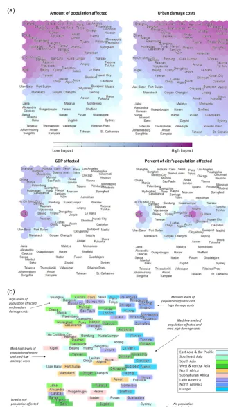
Patterns of urban flood conditions in 2010 are shown on the baseline map, SOM1, in Fig. 1. The placement of city la-bels indicates the relationship of each city to each other in terms of river flood impacts on population and urban dam-age costs. The map is created by organizing the cities with respect to each other based on both of these factors. Cities close together are more similar in the amount of population affected and urban damage costs, and cities located far apart are less similar.
The relative placement of the cities on the map is the main map characteristic providing insight into the features of the data, indicating differences in a combination of the vari-ables which can be discerned from the colouring of Fig. 1a. Each map node has a four-component vector (representing the value of each of the four variables at the location of the node in data space). The four images in Fig. 1a show SOM1’s city labels over grids coloured separately by the values of each of the four variables (white is low, purple is high). For each city, the relative value of each of the variables can be seen. For example, Cincinnati (top right) incurs high mate-rial damage costs and medium population affected, whereas Ulan Bator (middle left) has a similar population affected as Cincinnati but much lower material damage costs.
The nonlinearity of the relationships between the variables is evident from the colouring of the grids, indicating that high (or low) values are located on different regions of the map for each variable. The smooth transition of the values of each variable is also apparent by the smooth transition of colours along the grids. General information about the preva-lent baseline global patterns and the relative flood conditions in the specific cities can be gained from inspection of these map labels and coloured grids.
Each area of the grid represents a general pattern, or com-bination of variables in the data, some of which are indicated by annotations in Fig. 1b. In general, higher amounts of pop-ulation affected and urban damage costs resulting from river flooding are represented by areas towards the top of the map, and these variables decrease in value down the map. Values of affected population are lowest just in from the lower left corner and undulate along the bottom of the map, sweeping upwards to a maximum at the upper left corner. Urban
dam-age values are lowest in the lower left corner and increase in concentric arcs up to the upper right corner. Generally, the left of the map contains patterns involving higher impacts on populations than on property, and the right of the map higher impacts on property than on populations.
From Fig. 1b, relationships can be discerned between re-gions, as well as between cities in the same region. For in-stance, cities in north Africa, sub-saharan Africa, and west and central Asia are predominantly located in the lower por-tion of the map, corresponding to a prevalent pattern of low flood impacts on both population and property. Cities in southeast and south Asia generally correspond to the patterns of high impacts on population and property found in the up-per left of the map. Cities in Europe stretch from the top to the bottom of the map, ranging from high overall flood ef-fects (Paris) to no flood efef-fects at all (Thessaloniki). North American cities are matched to patterns that represent more significant impacts on property than on population (down the right side of the map), and are split between those with high property damages (Philadelphia, Los Angeles, etc. – in the top right) and those with low damages (St. Catherine’s – in the bottom right).
Impacts on GDP and the proportion of the cities’ popula-tions affected are shown in the two lower maps of Fig. 1a, though these variables were not used to position the cities on the map. Cities in which river-related urban flooding is esti-mated to highly affect the country’s GDP are coloured on the lower left map. Kigali, in particular, which incurs medium– high flood impacts, sees a large impact on Rwanda’s GDP, perhaps because Kigali is the main city in this relatively small country (Kreimer et al., 2003). GDP is most affected by flooding in the following cities: Kigali, Bangkok, Yere-van, Dhaka, Bamako, and Cairo. Cities in which the flood-affected population forms a significant proportion of the city’s population are coloured on the lower right map, pre-dominantly in a horizontal strip across the centre. The highest proportions are in Jequie (15 %), Kigali (7 %), Chinju (6 %), Le Mans (5 %), and Tacoma (3 %).
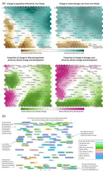
3.2 SOM2: projected changes in urban flood impacts (to 2030)
SOM2 identifies the projected patterns of evolving river flood conditions in the cities (between 2010 and 2030), based on city-specific projections of increasing or decreasing flood im-pacts on population and damage costs, and whether these changes are anticipated to be driven more by climate change or development (Fig. 2).
change. White represents a mid-range in which both climate change and development are predicted to impact future flood conditions relatively equally. Areas of the map representing patterns of increased flood impacts predominantly due to cli-mate change or development can be located in Fig. 2b.
Investigating SOM2, we see that climate change is pro-jected to be predominantly responsible for increases in pop-ulation vulnerability in all cities besides those in the top left corner (around Ho Chi Minh City). Climate change is an-ticipated to decrease flood damage costs in cities located at the bottom of the map (around Madrid), and decrease im-pacts on populations in cities in the mid-left (around Min-neapolis) and mid-lower (again around Madrid) portions of the map. Socioeconomic development is projected to be the main driver increasing flood damage costs in cities on the upper-left triangle of the map (roughly from Mumbai down to Tebessa). Only in Ho Chi Minh City is development antic-ipated to be almost completely responsible for all increases in river flood impacts; all other cities in this study are at least partially affected by climate change. Development is not pro-jected to play any part in a decrease in flood damage costs in any cities in this study (Caracas and Tebessa have no change in damage costs on the upper map, though it is attributed to development on the lower map).
Geographic regions are shown in Fig. 2b with coloured text backgrounds. Cities in Southeast Asia are mostly found at the top of the map indicating high projected increases in overall flood impacts. South Asian cities are mostly located in the two areas of the map with patterns of very high in-creases in flood impacts, split between those projected to be most affected by development (around Mumbai, top middle) and by climate change (around Puna, mid-right). Many north African cities are located in the lower left, indicating antici-pated reductions in flooding due to socioeconomic develop-ment. North American cities are spread across the middle of the map indicating a wide range of projected changes.
Climate change and development may lead to opposing changes in a city’s flood impacts on population and property. A number of cities in this data set are predicted to have af-fected populations decreasing due to climate change, whilst damage costs increase due to socioeconomic factors (around Springfield and Port Sudan, in the mid-left). A decrease in flood effects on urban damages due to climate change, but an increase in affected population largely due to development is, out of the cities in this study, only projected for Algiers (in the lower left portion of the map).
In some cities, both drivers may generate changes in the same direction. For instance, in Marrakech, Yulin, Yerevan, and Gorgan, climate change is projected to be responsible for a decrease in damage costs, whilst socioeconomic devel-opment is anticipated to play a major role in the decrease in affected population, suggesting that the reduction of pop-ulation vulnerability due to development is complementing the direction of change instigated by climate change. In cer-tain cities near the upper left of the map (Santiago, Zugdidi,
and Yiyang), an overall increase in flood impacts is expected, with increases in affected population almost completely at-tributed to climate change and increases in damage costs al-most completely attributed to development.
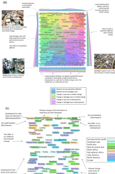
3.3 SOM3: temporal patterns
Relationships between the baseline characteristics and pro-jected future changes in urban flooding in the individual cities are shown in Figs. 1 and 2, respectively; however, po-tentially similar temporal patterns between the cities are not evident from these maps. To link the information abstracted from the first two maps, we create a temporal map, SOM3, shown in Fig. 3. SOM3 identifies which cities experience similar baseline flooding, are expected to incur comparable future hydrologic pressures from climate change and/or de-velopment, and are projected to respond in similar ways (or which cities may diverge in the future from similar baseline conditions).
The nodes of SOM3 are coloured based on the results of a second-level clustering, giving a visual separation to clusters of more similar data. Clusters are numbered from 1 to 16 for reference. As the cities have been located on SOM3 based on their locations on the “baseline” and “future projected changes” SOMs (in which the values of the variables vary smoothly though not monotonically along the axes), again the characteristics of the cities will flow smoothly along the map though multiple peaks and troughs of each variable are possible. The gradients of the cluster characteristics are indi-cated along the axes in Fig. 3a, which are nonlinear in data space.
Broad overviews of the patterns represented by certain re-gions of the map are identified in Fig. 3 with arrows. The largest increases in flood effects are generally represented by nodes in the lower half of the map, whilst the largest de-creases in flood effects are represented by nodes in the top left. Climate change is predicted to be the main driver of changes in population vulnerability along the top and down the left and right sides of the map, and in urban damages on the top and right of the map; therefore, climate change is the leading driver of changes in flood impacts on both population and damage costs at the top of the map. Development is the main driver of changes in flood impacts on populations in the lower and upper left side of the map, and on urban damages in the lower left area of the map; therefore, development is the leading driver of changes in flood impacts on both popu-lation and damage costs in cities on the lower left side of the map.
the cities of this region have differing baseline flood levels (as shown on SOM1), most are projected to incur some re-duction in future flood impacts (as shown on SOM2), with the exception of Cairo and Aswan. These cities both have forecasts of increased flood impacts – for Aswan increased impacts on the population due to climate change and impacts on property due to development, and for Cairo future impacts are projected to increase due to a relatively even mixture of both drivers. Another example can be seen in the cities of the USA shown on the map. They have similar starting condi-tions, yet are in two well-separated clusters on SOM3 – those around Houston and those around Los Angeles. The cities clustered around Houston are characterized by low impacts on population but high damage costs projected to elevate due to development, implying the possibility for local improve-ments through planning or mitigation strategies. The cities clustered around Los Angeles, however, are characterized by high overall impacts projected to increase predominantly due to climate change. In sub-saharan Africa we see Kigali and Bamako (which have similar medium–high baseline flood-ing conditions) are both expected to see increased impacts, but the cities are separated by SOM3 as these flood increases are attributed to development in Kigali and climate change in Bamako.
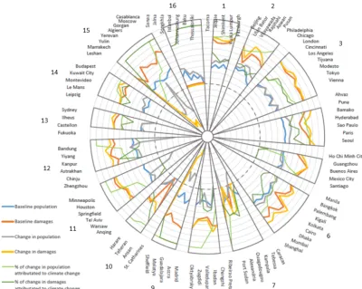
To further analyse the characteristics of each cluster and the patterns found on SOM3, the properties of each city in the 16 clusters are shown in a radial plot in Fig. 4. Baseline val-ues of population affected (blue, units are the number of peo-ple) and damages (orange, units are in USD) are shown on a symmetrical logarithmic scale ranging from−8 (i.e. signify-ing a value of −100 000 000) to 11 (100 000 000 000) with the region between−1 and 1 on the plot set as linear to avoid logarithmic discontinuities in the vicinity of zero. Zero is in-dicated by a dashed circumference, and each progressive ring is an exponentially higher (or lower) value. Changes in popu-lation affected and damage costs are shown on the same scale in grey and yellow, respectively. Values inside the dashed circle (zero) represent decreases in flood impacts, and val-ues outside represent increases, with the size of the increase or decrease indicated by the distance from the dashed cir-cle. The influence of climate change is shown (light green for population and dark green for damages) on a linear scale from the same zero circumference, in units of “percentage of projected change attributable to climate change” (each pro-gressive ring is 10 %). Green lines closer to the outer ring than the centre therefore indicate that the flood impacts on the city are anticipated to be more influenced by climate change than by development. If the green lines are both in the mid-dle of the segment, this indicates a relatively equal influence of both drivers on both population and property. Diverging green lines indicate that either population or damage costs are more influenced by climate change, and the other by de-velopment.
From Fig. 4, we can see the differences between neigh-bouring clusters, such as 10 and 16 located in the top right
of the map. Both clusters are characterized by low base-line impacts of flooding on the population, with small in-creases in population impacts projected primarily due to cli-mate change. However, cities in cluster 16 incur no flood damage costs at all in the baseline or future cases, yet in clus-ter 10 damage costs are projected to increase due to climate change and development. Therefore, development has little or no impact on cities in cluster 16 but does play a role in the increase in damages in cluster 10. In the top left of SOM3, we can now also discern the difference between clusters 9 and 15. In both clusters, development is projected to have no impact on the reduction of flood damage costs in most cities. Development does, however, play a strong role in the reduc-tion of flood impacts on populareduc-tions in cluster 15 (except for Moscow and Casablanca) but none on populations in clus-ter 9.
The relationship between the two drivers, climate change and development, can be discerned from Figs. 3 and 4. Cli-mate change is projected to impact populations more than ur-ban damage costs in clusters stretched across the centre of the map (clusters 8, 11, 5, 6, 12, 14, 1, 10, 1, 2, and 4 – in cities in these clusters, the proportion of change in the population af-fected attributed to climate change is higher than the propor-tion of change in damage costs attributed to climate change). In cluster 15, the population is projected to be more influ-enced by development than damage costs will be (a higher proportion of the change in damage costs is attributed to cli-mate change than for population). In the remaining clusters, climate change (and development) are projected to affect the population and damage costs relatively similarly (clusters 7, 13, 9, 16 and 3). Some examples of diverging impacts on population and damage costs stand out on the radial plot in Fig. 4. For instance, in Port Sudan, Sheffield, and Bandung, significant reductions in affected population are projected to be 100 % due to climate change; however, large projected increases (∼300 to 400 %) in damages are due mostly to de-velopment. In Leshan, development is projected to slightly lower the amount of affected population and also to increase damage costs more than 3-fold.
4 Discussion
Figure 4.Radial plot of clusters of Fig. 3 – the city members of the 16 clusters of Fig. 3 are shown with their individual variable values. The scale is logarithmic for baseline and changes in population and damages, and linear for the percent of change attributed to climate change, with the dashed circle representing zero.
is provided. The information that can be gleaned from the SOMs is related to information in current literature through the use of specific examples.
The lower left region of SOM3 highlights the fact that a number of cities already experiencing large flood effects are anticipated to incur great flood increases influenced pre-dominantly by socioeconomic factors. In these cities, climate change is playing a large role, and yet it is overshadowed by the magnitude of regional economic growth (UNEP, 2016; Scientific American, 2018) leading to migration, changing land use, and unplanned development in flood zones. Many of these cities are in Asia, where the climate is experienc-ing warmexperienc-ing trends, increasexperienc-ing temperature and precipitation extremes, and rapid glacial melting resulting from climate change (Pachauri et al., 2014, chapter 24: “Asia”). However, it can be seen that socioeconomic growth in this area is pro-jected to have even more of an impact on urban floods than climate change.
Pachauri et al. (2014, chapter 24: “Asia”) assert that hu-man and material losses due to flooding are already heavily concentrated in India, Bangladesh, and China and Jongman et al. (2012) estimate the largest current and future economic
large increases, 50–75 % of which are attributed to devel-opment), and Ho Chi Minh City (with a 50 % increase in affected population and an over 5-fold increase in damage costs, almost entirely attributed to development).
On SOM3, we can identify that developmental changes in some cities appear to be effectively reducing impacts from river flooding, for example in Marrakech (cluster 15). The affected population level is projected to decrease mostly due to socioeconomic factors (World Resources Institute’s Aque-duct Global Flood Analyzer Tool, 2018; Ward et al., 2013; Winsemius et al., 2013). Through an “Integrated Disaster Risk Management and Resilience Program for Morocco” (World Bank, April 2016–December 2021), Morocco is be-coming more resilient to climate change and less vulnerable to natural hazards, and is ensuring a rapid transition to a low-carbon economy. Through Morocco’s national strategy for sustainable development, a commitment has been made to reduce national greenhouse gas emissions by 32 % by 2030. This will be done through an increase in renewable energy sources to 50 %, a reduction in energy consumption by 15 %, as well as various agricultural, water, waste, forest, industry, and housing initiatives (United Nations Framework Conven-tion on Climate Change, 2018). These housing initiatives in Marrakech include a slum clearance and relocation project, which has become part of urban policy (Ibrahim, 2016), re-ducing the amount of people inhabiting flood hazard zones. Alert systems in the valleys of the Atlas Mountains region above Marrakech have been improved, and the proportion of the population living in slums has decreased from over 8 % in 2004 to less than 4 % in 2010 (UN-Habitat, 2014). The urbanization rate in Morocco is also projected to slow down towards 2030 (UN-Habitat website). This risk-prevention ap-proach combining early warning systems, relocation of in-habitants out of the flood zone, and less urban expansion is expected to combine to reduce the impact of floods on the population of Marrakesh.
Current high flood impact conditions projected to get much greater primarily due to climate change are anticipated for cities in the lower right of SOM3, with high magnitude changes expected for impacts on both population and prop-erty. One of these cities, Sao Paulo, is expected to experience an almost 7-fold increase in both the number of population affected (to over 140 000 annually) and urban damage costs (to over USD 500 000 000 annually) by 2030. Some 15 % of the change in population and 35 % of the change in dam-ages is attributed to development, but the majority of the change is projected to come from climate change. Sao Paulo, the largest city in Brazil, has a city footprint projected to in-crease over 38 % by 2030, by which time 22 % of the urban area may be located in flood zones (Young, 2013). The IPCC (Pachauri et al., 2014 chapter 14: “Latin America”) predicts the increase in temperature in central and south Brazil to be the largest projected increase in Latin America, which will be combined with a 10–15 % increase in autumnal precipita-tion, greatly affecting the hydrologic cycle in the region. The
substantial change in development is therefore expected to be eclipsed by the even greater projected change in climate in Sao Paulo, and other cities in this region of SOM3.
The anticipated reduction in flood damage costs caused by climate change evident in cluster 15 may be a result of chang-ing snowmelt conditions upstream of these cities. It has been shown that some global regions will experience a decreasing trend in the magnitude and frequency of snowmelt floods as the climate warms, as well as a shift in the timing of these floods (Schiermeier, 2011; Barnett et al., 2005; Immerzeel et al., 2010).
Many high-income cities with already high flood vulnera-bilities have projections for large elevations in damage costs, but not increased levels of affected population. This can be seen in cities in SOM3 centred around London, Tokyo, Los Angeles, and Vienna (cluster 3), and Sydney and Castellon (cluster 13). Through high levels of planning, preparedness, and infrastructure, prosperous regions generally have sys-tems in place to minimize flood impacts on the population, even though they may incur large economic losses (Desai et al., 2015; Kreimer et al., 2003). Almost half of the projected increases in these clusters are attributed to development, sug-gesting that these cities may have the capacity for lessening potentially elevated flood damage costs by concentrating on planning and mitigation policies.
Although changing climate in some areas is projected to lessen regional flooding, development within urban flood zones may be severe enough to offset any reductions in flood impacts. This can be seen most prominently in a strip on the left of SOM3 stretching from Port Sudan down to Santiago.
Although this study does not consider coastal flooding, it may be noted that due to their locations near river mouths, many of the cities in the lower left of the map that are pro-jected to experience high increases in impacts from river flooding are also at risk of increased coastal flooding from intensified storms and sea level rise due to climate change. Mumbai, Guangzhou, Shanghai, Ho Chi Minh City, Kolkata, Bangkok, and Dhaka are 7 of the top 14 cities (out of 136) ranked by current population exposure to coastal flooding. These same cities also comprise the top 7 cities (in the order Kolkata, Dhaka, Mumbai, Guangzhou, Ho Chi Minh City, Shanghai, Bangkok) ranked by future (2070) estimated pop-ulation exposed to coastal flooding (UNEP, 2016; Nicholls et al., 2008).
costs. This supports the findings of Milly et al. (2002) who observed that the frequency of large flood events in large basins had increased substantially in the 20th century, but smaller floods had not.
The analysis in this paper is solely based on the data pro-vided in Aqueduct, regardless of the extent to which on-the-ground flood management measures are incorporated into the socioeconomic models which produced these data. A dis-cussion characterizing individual cities is included here as a point of interest to relate the data to current national con-ditions, providing possible reasons why these cities may fit into the map where they do.
5 Conclusion
This study adds to the understanding of natural hazards in a global context, an important aspect of regional disaster risk management due to the dependency of local situations on global processes (Desai et al., 2015). Complex, nonlinear social–environmental relationships make it difficult to antic-ipate local responses to global changes (Desai et al., 2015), and this study contributes to risk communication (the process between risk perception and adaptation planning; Cardona et al., 2012) providing a visual analysis of global patterns of evolving flood impacts, socioeconomic development, and cli-mate change, and the local city-level consequences of these changes.
Global patterns of urban flood responses to global and lo-cal changes in hydrology driven by climate change and de-velopment have been identified and visually communicated through a series of related SOMs. Cities have been matched to these global patterns, and relationships between the in-dividual cities have been discerned with respect to baseline flooding conditions and expected future changes. The visual analysis in this study has revealed interesting city-level pat-terns that are otherwise unobservable in the complex data set, and provides a comparison and distinction between individ-ual cities that is not apparent in regional- or economic-level projections.
We have performed dimension reduction and clustering with a series of SOMs to identify changing global patterns of city-level flood risks. The maps provide an indication of the predominant characteristics which determine the differences in urban river flood impacts between cities, and the cities occupy positions on the maps signifying their relative con-ditions. The method used here incorporates adaptions to the SOM technique for map shape selection and temporal pattern extraction, allowing two levels of information to emerge: the characteristic patterns of dynamic global urban flood vulner-abilities and a comparison between the cities with respect to flood characteristics and trends. This SOM method could be adopted for visualizing and clustering any large data set in which the underlying inter-variable relationships are diffi-cult to explicitly define, and which change over time such as
is common with human–environmental interactions. The re-sulting visualizations produce an overall impression of the temporal structure and clusters in the data, allowing for a readily understood overview of the relationships between the variables, and amongst individual data items.
A shortcoming of the method used in this study is the as-signment of flood protection level based on an assumption of proportionality with national income level. As standard-ized, current information on the real flood protection levels of all the cities in the data set is not readily available, this assumption has been necessary and has been made in line with current practice. This limitation has been recently ac-knowledged in the literature, with Winsemius et al. (2016) noting that “currently installed flood protection is an impor-tant missing link in the assessment of global flood risk”. Fu-ture studies may aim to include specific flood protection lev-els for each city.
Whilst the timeline of this study is short, it is restricted by the data that is available. Studies on a global scale have been traditionally limited due to a lack of cohesive data sets, and therefore the data set provided by Aqueduct is valuable for the fact that it spans a global set of cities and provides a rare opportunity for comparison. As the data is only pro-vided for 2010 and 2030, there was no prospect for a longer analysis. Whilst this analysis may not provide a long-term outlook, at the very least an important insight into current and near-future conditions can be gained.
Cities have major implications for climate change mitiga-tion and adaptamitiga-tion (Revi et al., 2014). Unplanned develop-ment and urban migration are increasing vulnerabilities to natural hazards (UNEP, 2016) and land cover change and greenhouse gas emissions are intensifying urban hydrology. Understanding the relationship between flood impacts and social vulnerability is a necessary step for prioritizing flood mitigation and prevention strategies (Doocy et al., 2013). Whether the main driver of increased urban flood impacts is development or climate change, cities will benefit from de-velopment restrictions and planning standards for urban ex-pansion, sustainable land development, management of pop-ulation distribution and migration, and early warning systems and preparedness (Revi et al., 2014; UN-DESA, 2015; Doocy et al., 2013).
Data availability. Flood impact data for this study are available at the World Resource Institute’s Aqueduct Global Flood Ana-lyzer tool. City population data (2010) and future population es-timates (2030) are available from the UN Department of Economic and Social Affairs (UN-DESA, 2015), and GDP per country from the World Bank’s World Development Indicators database (http: //data.worldbank.org/data-catalog/world-development-indicators).
Competing interests. The authors declare that they have no conflict
of interest.
Edited by: Elena Toth
Reviewed by: Rolf Larsson and one anonymous referee
References
Agarwal, P. and Skupin, A.: Self-organising maps: Applications in geographic information science, John Wiley & Sons, 2008. Angel, S., Parent, J., Civco, D., and Blei, A.: Atlas of Urban
Expan-sion, Lincoln Institute of Land Policy, Cambridge, MA, 2010a. Angel, S., Parent, J., Civco, D., Blei, A., and Potere, D.: A Planet
of Cities: Urban Land Cover Estimates and Projections for All Countries, 2000–2050, Lincoln Institute of Land Policy Working Paper, Cambridge, MA, 2010b.
Atlas of Urban Expansion: http://www.lincolninst.edu/subcenters/ atlas-urban-expansion/Default.aspx, last access: July 2016. Barnett, T., Adam, J. and Lettenmaier, D.: Potential impacts of a
warming climate on water availability in snow-dominated re-gions, Nature, 438, 303–309, 2005.
Cardona, O.-D., van Aalst, M. K., Birkmann, J., Fordham, M., Mc-Gregor, G., and Mechler, R.: Determinants of risk: exposure and vulnerability, 2012.
Clark, S., Sarlin, P., Sharma, A., and Sisson, S. A.: Increasing de-pendence on foreign water resources? An assessment of trends in global virtual water flows using a self-organizing time map, Ecol. Inform., 26, 192–202, 2015.
Clark, S., Sisson, S. A., and Sharma, A.: A dimension range rep-resentation (DRR) measure for self-organizing maps, Pattern Recog., 53, 276–286, 2016.
Clark, S., Sisson, S. A., and Sharma, A.: Nonlinear manifold repre-sentation in natural systems, Environ. Model. Softw., 89, 61–76, 2017.
Cunderlik, J. M. and Ouarda, T.: Trends in the timing and magnitude of floods in Canada, J. Hydrol., 375, 471–480, 2009.
Davies, D. L. and Bouldin, D. W.: A cluster separation measure, IEEE T. Pattern Anal. Mach. Intel., 2, 224–227, 1979.
Desai, B., Maskrey, A., Peduzzi, P., De Bono, A., and Herold, C.: Making Development Sustainable: The Future of Disaster Risk Management, Global Assessment Report on Disaster Risk Reduction, United Nations Office for Disaster Risk Reduction, Geneva, Switzerland, 2015.
Doocy, S., Daniels, A., Murray, S., and Kirsch, T. D.: The human impact of floods: A historical review of events 1980–2009 and systematic literature review, PLoS Curr., 16, 12, 2013.
Frich, P., Alexander, L. V., Della-Marta, P., Gleason, B., Haylock, M., Tank, A., and Peterson, T.: Observed coherent changes in climatic extremes during the second half of the twentieth century, Clim. Res., 19, 193–212, 2002.
Ibrahim: Slum eradication policies in Marrakech, Morocco, World Bank Conference on Land and Poverty, Washington, D.C., 2016. Immerzeel, W. W., Van Beek, L. P. H., and Bierkens, M. F. P.: Cli-mate change will affect the Asian water towers, Science, 328, 1382–1385, 2010.
ISIMIP: https://www.pik-potsdam.de/research/ climate-impacts-and-vulnerabilities/research/
rd2-cross-cutting-activities/isi-mip/about, last access: Febru-ary 2018.
Jongman, B., Ward, P. J., and Aerts, J. C.: Global exposure to river and coastal flooding: Long term trends and changes, Global En-viron. Change, 22, 823–835, 2012.
Jongman, B., Winsemius, H. C., Aerts, J. C., de Perez, E. C., van Aalst, M. K., Kron, W., and Ward, P. J.: Declining vulner-ability to river floods and the global benefits of adaptation, P. Natl. Acad. Sci. USA, 112, E2271–E2280, 2015.
Kaski, S. and Kohonen, T.: Exploratory data analysis by the self-organizing map: Structures of welfare and poverty in the world. Neural networks in financial engineering, in: Proceedings of the third international conference on neural networks in the capital markets, 1996.
Kiviluoto, K.: Topology preservation in self-organizing maps, in: IEEE International Conference on Neural Networks, 1996. Kohonen, T.: Self-organizing maps, in: Vol. 30 of Series in
Infor-mation Sciences, Springer, Berlin, 2001.
Kohonen, T.: Essentials of the self-organizing map, Neural Netw., 37, 52–65, 2013.
Kreimer, A., Arnold, M., and Carlin, A.: Building safer cities: the future of disaster risk, World Bank Publications, 2003.
Kummu, M., De Moel, H., Ward, P. J., and Varis, O.: How close do we live to water? A global analysis of popula-tion distance to freshwater bodies, PLoS One, 6, e20578, https://doi.org/10.1371/journal.pone.0020578, 2011.
Kunkel, K. E., Pielke Jr., R. A., and Changnon, S. A.: Temporal fluctuations in weather and climate extremes that cause economic and human health impacts: A review, B. Am. Meteorol. Soc., 80, 1077, https://doi.org/10.1175/1520-0477(1999)080<1077:TFIWAC>2.0.CO;2, 1999.
Meehl, G. A., Arblaster, J. M., and Tebaldi, C.: Under-standing future patterns of increased precipitation inten-sity in climate model simulations, Geophys. Res. Lett., 32, https://doi.org/10.1029/2005GL023680, 2005.
Mills, G.: Cities as agents of global change, Int. J. Climatol., 27, 1849–1857, 2007.
Milly, P. C. D., Wetherald, R. T., Dunne, K. A., and Delworth, T. L.: Increasing risk of great floods in a changing climate, Nature, 415, 514–517, 2002.
Muis, S., Güneralp, B., Jongman, B., Aerts, J. C., and Ward, P. J.: Flood risk and adaptation strategies under climate change and urban expansion: A probabilistic analysis using global data, Sci. Total Environ., 538, 445–457, 2015.
Nature: Waters encroaching, Nat. Clim. Change, 6, 635, 2016. Nicholls, R. J., Hanson, S., Herweijer, C., Patmore, N., Hallegatte,
S., Corfee-Morlot, J., and Muir-Wood, R.: Ranking port cities with high exposure and vulnerability to climate extremes, 2008. Pachauri, R. K., Allen, M. R., Barros, V. R., Broome, J., Cramer,
assess-ment report of the Intergovernassess-mental Panel on Climate Change, IPCC, p. 151, 2014.
Revi, A., Satterthwaite, D. E., Aragón-Durand, F., Corfee-Morlot, J., Kiunsi, R. B. R., Pelling, M., Roberts, D. C., and Solecki, W.:Urban areas, in: Climate Change 2014: Impacts, Adaptation, and Vulnerability. Part A: Global and Sectoral Aspects, Contri-bution of Working Group II to the Fifth Assessment Report of the Intergovernmental Panel on Climate Change, Cambridge Univer-sity Press, Cambridge, UK and New York, NY, USA, 2014. Samir, K. C. and Lutz, W.: The human core of the shared
socioe-conomic pathways: Population scenarios by age, sex and level of education for all countries to 2100, Global Environ. Change, 42, 181–192, 2014.
Schiermeier, Q.: Increased flood risk linked to global warming, Na-ture, 470, 316–317, 2011.
Shanmuganathan, S., Sallis, P., and Buckeridge, J.: Self-organising map methods in integrated modelling of environmental and economic systems, Environ. Model. Softw., 21, 1247–1256, https://doi.org/10.1016/j.envsoft.2005.04.011, 2006.
Shared Socioeconomic Pathways: https://tntcat.iiasa.ac.at/SspDb/ dsd?Action=htmlpage&page=about (last access: July 2016), 2018.
Sheppard, S. R. J.: Landscape visualisation and climate change: the potential for influencing perceptions and behaviour, Environ. Sci. Policy, 8, 637–654, 2005.
Scientific American: https://www.scientificamerican.com/article/ extreme-rain-may-flood-54-million-people-by-2030/ (last ac-cess: July 2016), 2018.
Skupin, A. and Hagelman, R.: Visualizing demographic trajectories with self-organizing maps, GeoInformatica, 9, 159–179, 2005. Sofia, G., Roder, G., Dalla, F. G., and Tarolli, P.: Flood dynamics in
urbanised landscapes: 100 years of climate and humans’ interac-tion, Scient. Rep., 7, 40527, https://doi.org/10.1038/srep40527, 2017.
SOM Toolbox: http://www.cis.hut.fi/somtoolbox (last access: July 2016), 2018.
Ultsch, A.: U-matrix: a tool to visualize clusters in high dimensional data, Fachbereich Mathematik und Informatik, Marburg, 2003. UN-DESA: World Urbanization Prospects: The 2014 Revision,
United Nations Department of Economic and Social Affairs, New York, NY, USA, 2015.
UNEP: Summary of the sixth global environment outlook regional assessments: Key findings and policy messages, United Na-tions Environment Programme, http://wedocs.unep.org/handle/ 20.500.11822/7644 (last access: March 2018), 2016.
United Nations Framework Convention on Climate Change: http: //www4.unfccc.in (last access: July 2016), 2018.
UN-Habitat: State of the world’s cities 2010/2011: bridging the ur-ban divide, EarthScan, 2010.
UN-Habitat: Urban Equity in Development – Cities for Life, World Urban Forum, 7 April 2014, Medellin, Colombia, 2014. Václavík, T., Lautenbach, S., Kuemmerle, T., and Seppelt, R.:
Map-ping global land system archetypes, Global Environ. Change, 23, 1637–1647, 2013.
Vesanto, J. and Alhoniemi, E.: Clustering of the self-organizing map, IEEE T. Neural Netw., 11, 586–600, https://doi.org/10.1109/72.846731, 2000.
Ward, P. J., Jongman, B., Sperna Weiland, F., Bouwman, A., van Beek, R., Bierkens, M. F. P., Ligtvoet, W., and Win-semius, H. C.: Assessing flood risk at the global scale: model setup, results, and sensitivity, Environ. Res. Lett., 8, 044019, https://doi.org/10.1088/1748-9326/8/4/044019, 2013.
Ward Jr., J. H.: Hierarchical grouping to optimize an objective func-tion, J. Am. Stat. Assoc., 58, 236–244, 1963.
Wasko, C. and Sharma, A.: Steeper temporal distribution of rain intensity at higher temperatures within Australian storms, Nat. Geosci., 8.7, 527–529, 2015.
Wentz, F. J., Ricciardulli, L., Hilburn, K., and Mears, C.: How much more rain will global warming bring?, Science, 317, 233–235, 2007.
Willems, P., Olsson, J., Arnbjerg-Nielsen, K., Beecham, S., Pathi-rana, A., Gregersen, I. B., and Madsen, H. (Eds.): Impacts of climate change on rainfall extremes and urban drainage systems, IWA publishing, 2012.
Winsemius, H. C., Van Beek, L. P. H., Jongman, B., Ward, P. J., and Bouwman, A.: A framework for global river flood risk assessments, Hydrol. Earth Syst. Sci., 17, 1871–1892, https://doi.org/10.5194/hess-17-1871-2013, 2013.
Winsemius, H. C., Aerts, J. C., van Beek, L. P., Bierkens, M. F., Bouwman, A., Jongman, B., Kwadijk, J. C., Ligtvoet, W., Lucas, P. L., van Vuuren, D. P., and Ward, P. J.: Global drivers of future river flood risk, Nat. Clim. Change, 6, 381, 2016.
World Bank’s World Development Indicators database: http://data. worldbank.org/data-catalog/world-development-indicators (last access: July 2016), 2018.
World Resources Institute’s Aqueduct Global Flood Analyzer Tool: http://floods.wri.org/#/ (last access: July 2016), 2018.
World Resources Institute’s Aqueduct Global Flood Risk Country Rankings: http://www.wri.org/resources/data-sets/ aqueduct-global-flood-risk-country-rankings (last access: July 2016), 2018.