www.hydrol-earth-syst-sci.net/19/2925/2015/ doi:10.5194/hess-19-2925-2015
© Author(s) 2015. CC Attribution 3.0 License.
TopREML: a topological restricted maximum likelihood approach
to regionalize trended runoff signatures in stream networks
M. F. Müller and S. E. Thompson
Department of Civil and Environmental Engineering, Davis Hall, University of California, Berkeley, CA, USA Correspondence to: M. F. Müller (marc.f.muller@gmail.com)
Received: 12 December 2014 – Published in Hydrol. Earth Syst. Sci. Discuss.: 29 January 2015 Revised: 01 May 2015 – Accepted: 03 June 2015 – Published: 24 June 2015
Abstract. We introduce topological restricted maximum likelihood (TopREML) as a method to predict runoff sig-natures in ungauged basins. The approach is based on the use of linear mixed models with spatially correlated ran-dom effects. The nested nature of streamflow networks is taken into account by using water balance considerations to constrain the covariance structure of runoff and to account for the stronger spatial correlation between flow-connected basins. The restricted maximum likelihood (REML) frame-work generates the best linear unbiased predictor (BLUP) of both the predicted variable and the associated prediction uncertainty, even when incorporating observable covariates into the model. The method was successfully tested in cross-validation analyses on mean streamflow and runoff frequency in Nepal (sparsely gauged) and Austria (densely gauged), where it matched the performance of comparable methods in the prediction of the considered runoff signature, while significantly outperforming them in the prediction of the as-sociated modeling uncertainty. The ability of TopREML to combine deterministic and stochastic information to generate BLUPs of the prediction variable and its uncertainty makes it a particularly versatile method that can readily be applied in both densely gauged basins, where it takes advantage of spa-tial covariance information, and data-scarce regions, where it can rely on covariates, which are increasingly observable via remote-sensing technology.
1 Introduction
Regionalizing runoff and streamflow for the purposes of making predictions in ungauged basins (PUB) continues to be one of the major contemporary challenges in hydrology.
At global, regional and local scales only a small fraction of catchments are monitored for streamflow (Blöschl et al., 2013), and this fraction is at risk of decreasing given the ongoing challenge of maintaining existing gauging stations (Stokstad, 1999). Reliable information about local stream-flows is essential for the management of water resources, es-pecially in the context of changing climate, ecosystem and demography; flow prediction uncertainties are bound to prop-agate and lead to significantly suboptimal design and man-agement decisions (e.g., Sivapalan et al., 2014). Techniques are needed to maximize the use of available data in data-scarce regions to accurately predict streamflow, while pro-viding a reliable estimate of the related modeling uncertainty.
1.1 Linear models
There are a number of approaches to predicting runoff in un-gauged catchments, including process-based modeling (e.g., Müller et al., 2014), graphical methods based on the con-struction of isolines (e.g., Bishop and Church, 1992), and statistical approaches. Statistical approaches are often imple-mented via linear regression, wherein the runoff signature of interest is considered to be an unobservable random variable correlated with observable features of both gauged and un-gauged basins (e.g., rainfall, topography). Such linear mod-els are well understood and widely implemented, not only for PUB (see review in Blöschl et al., 2013, p.83) but also across a wide variety of fields in the physical and social sci-ences (e.g., Myers, 1990).
X of observed features then the linear model has the form:
y=Xτ+η. (1)
Hereτ is an a priori unknown set of weights that represent the influence of each external trend on the hydrological out-come being modeled. The residuals,η, are the observed vari-ation ofythat cannot be explained by a linear relation with X. If the residuals are independent and identically distributed (iid), the best linear unbiased predictions (BLUP) of bothy and its uncertainty (i.e., Var(y)) can readily be obtained us-ing ordinary least squares (OLS) regression. Unfortunately, residuals are rarely iid in hydrological applications due to the spatial organization of hydrological processes around the topology of river channel networks. This organization has the potential to introduce non-random spatial correlations with a structure imposed by the river network. To recover a suitable model in which residuals remain independent requires that the model structure be altered to explicitly account for the spatial and topological correlation in the residuals.
1.2 Spatial correlation models
There are several techniques available to address spatially correlated data. Within PUB, kriging-based geostatistical methods (Cressie, 1993) have been widely used (e.g., Huang and Yang, 1998; Gottschalk et al., 2006; Sauquet, 2006; Sauquet et al., 2000; Skøien et al., 2006). In a geostatisti-cal framework, a parametric function is used to model the relationship between distance and covariance in observa-tions. The ensuing semi-variogram is assumed to be homoge-nous in space, and predictions at a point are computed as a weighted sum of the available observations. The weights are chosen to minimize the variance while meeting a given con-straint on the expected value of the prediction. In ordinary kriging for PUB applications, this given constraint is sim-ply the average of the streamflow signature as observed in gauged catchments. Ordinary kriging can also be extended as “universal kriging” to include a linear combination of observable features (Olea, 1974). Kriging approaches are widely used to predict spatially distributed point-scale pro-cesses like soil properties (e.g., Goovaerts, 1999) and cli-matic features (e.g., Goovaerts, 2000). Although ordinary kriging has also been used to interpolate runoff (e.g., Huang and Yang, 1998), the theoretical justification for this ap-proach is less robust than for point-scale processes. Runoff is organized around a topological network of stream channels, and the covariance structure implied for prediction should reflect the higher correlation between streamflow at water-sheds that are “flow connected” (i.e., share one or more sub-catchments), compared to unconnected but spatially proxi-mate catchments. Currently, two broad classes of geostatis-tical methods accommodate this network-aligned correlation structure.
The first suite of methods posits the existence of an un-derlying point-scale process, which is assumed to have a
spatial auto-correlation structure that allows kriging to be applied. Because the runoff point-scale process is only ob-served as a spatially integrated measure made at specific gauged locations along an organized network of streams, the spatial auto-correlation structure of the point-scale pro-cess cannot itself be observed. Block-kriging approaches (Gottschalk et al., 2006; Sauquet, 2006; Sauquet et al., 2000) infer the semi-variogram of the (unobserved) point scale so as to best reproduce the observed spatial correlation of the area-integrated runoff at the gauges – a procedure known as regularization. The topology of the network is implicitly ac-counted for by the fact that nested catchments have over-lapping areas, which affect the relation between observed (area integrated) and modeled (point-scale) covariances. Yet, complex catchment shapes complicate the regularization of semi-variograms, meaning that the estimation of the point-scale process becomes analytically intractable and requires a trial-and-error approach in most practical applications (e.g., Top-kriging; Skøien et al. (2006)). Top-kriging is an ex-tension of the block-kriging approach that accommodates non-stationary variables and short observation records. Top-kriging provides an improved prediction method for hydro-logical variables when compared to ordinary kriging or lin-ear regression techniques (Laaha et al., 2014; Viglione et al., 2013; Castiglioni et al., 2011) and was recently extended to account for deterministic trends (Laaha et al., 2013). Top-kriging represents an important advance for PUB, but it does have a few drawbacks: (i) the regularization process is un-intuitive, and requires extensive trial-and-error to determine both the form of a suitable point-scale variogram, and its pa-rameters; (ii) this trial-and-error process is likely to be com-putationally expensive; (iii) like all kriging techniques, the estimation of the variogram is challenging when account-ing for observable features: the presence of an unknown trend coefficient and variogram leads to an underdetermined problem, making consistent estimates for both challenging. Cressie (1993, p. 166) showed that the presence of a trend tends to impose a spatially inhomogeneous, negative bias on the estimated semi-variogram. The bias increases quadrati-cally with distance, meaning that estimates of the long-range variance (the sill) are strongly impacted by the presence of the trend, leading to an underestimation of the prediction un-certainty. This bias, however, only marginally affects the pre-diction itself.
un-like Euclidian distances, the streamwise distance does not have the necessary properties to provide a solvable kriging system. This issue is addressed in Cressie et al. (2006) and Ver Hoef and Peterson (2010), where streamflow is mod-eled as a random process represented by a Brownian mo-tion that starts at the trunk of the tree (i.e., the river mouth) moves upstream, bifurcates and evolves independently on each branch. The resulting model only allows spatial depen-dence with points that are upstream on the river network and provides a positive definite covariance matrix that is estimated through restricted maximum likelihood (REML). Models of this nature have been successfully tested on stream chemistry data (Ver Hoef et al., 2006) and further developed to also allow spatial auto-correlation among random vari-ables on stream segments that do not share flow, with po-tential applications to the modeling of the concentration of upstream moving species (e.g., fishes or insects) (Ver Hoef and Peterson, 2010). While these methods do not account for the streamflow generation process, they avoid the conceptual and prediction uncertainty challenges confronted by kriging techniques.
1.3 The topological restricted maximum likelihood approach
Inspired by both types of approaches, here we present a method based on the use of linear mixed models to generate a BLUP for hydrological variables on a flow network. Rather than using a kriging estimator, we adopt a REML framework (Gilmour et al., 2004; Patterson and Thompson, 1971; Lark et al., 2006) to estimate variance parameters. This reduces the bias on the semi-variogram by allowing the variance to be estimated independently from the trend coefficients (Cressie, 1993; Lark et al., 2006). This use of a REML framework to estimate a linear mixed effect model on a topological sup-port is termed topological restricted maximum likelihood (TopREML). The approach is based on the following con-ceptual assumptions:
– Flow generation and propagation: similar to Top-kriging, runoff is assumed to be generated at a point scale on the landscape, from where it is routed to a channel and measured at a gauge (Fig. 1i). Runoff ob-servations made at any individual gauge (Fig. 1ii) can be broken up into a local contribution, derived from a never previously gauged catchment area, and an stream contribution that was previously observed at up-stream gauge(s) along the channel (Fig. 1iii). TopREML disaggregates all flow contributions into a cascade of lo-cal components, as observed at each successive gauge, and uses these characteristics to constrain the covari-ance structure of runoff and to account for the stronger spatial correlations between flow-connected basins. – Treatment of time: for the local effects to form a
suit-able basis for spatial interpolation, variations associated
with temporal correlation (e.g., travel time effects) need to be removed. This is achieved by considering time-averaged streamflow data, with the proviso that the time averaging window is much greater than the character-istic catchment and channel response timescales. This treatment of time has several specific consequences. First, TopREML is only suitable for the regionaliza-tion of time-averaged and statistically staregionaliza-tionary runoff properties (i.e., runoff signatures). Stationarity is neces-sary to ensure that the water balance assumption used to separate local from upstream runoff contributions is valid. However, as a consequence, TopREML cannot be used to interpolate transient signatures, such as those as-sociated with real-time forecasting. Nor can it be used to describe runoff properties that are correlated over timescales larger than the time averaging window. Be-cause of the stationarity assumption applied, all corre-lation arguments described in this manuscript refer to the spatial, and not temporal, correlation of the runoff signatures.
– Network topology: network topology in TopREML also follows a conceptual model that is similar to the model posited by Top-kriging. Topology is conceptu-alized by area connectivity. That is, flow-connected gauges are characterized by overlapping drainage ar-eas. Unlike Top-kriging, TopREML does not require in-formation about a spatially random point process, but solely relies on information measured at the gauges. It uses the inter-centroidal Euclidian distance between drainage areas of the local flow contributions at each gauge – the isolated drainage areas (IDA) – as a dis-tance metric to compute streamflow correlation. The underlying assumption is that runoff signatures of lo-cal flow generation regions that are close to each other (in Euclidian space) are more likely to be identical. Although TopREML does not require that the charac-teristics of a point-scale runoff generation process are known in order to support interpolation (a necessary re-quirement for Top-kriging), the existence of such a point process is consistent with the treatment of spatial corre-lation in TopREML. To illustrate this consistency, a styl-ized example relating point-scale runoff generation to the existence of a covariance structure that relates flow-connected gauges is outlined in Appendix A.
1.4 Paper outline
A B
C
t q
A B
C
A’ B’
C’
[image:4.612.127.466.66.207.2](i) (ii) (iii)
Figure 1. Conceptual flow propagation model. (i) Runoff is generated continuously by a spatially distributed point process and drained to
the stream network. (ii) When monitored by stream gauges, runoff is spatially integrated over the corresponding catchment and temporally averaged at the chosen observation frequency (e.g., daily streamflow). (iii) The model conceptualizes the catchments as isolated drainage areas (IDA) (A0, B0, and C0) representing the local runoff contribution to each gauge. The flow actually measured at each gauge is the sum of the upstream IDA.
(sparse gauges, significant trends) and Austria (dense gauge network, no observed trends). In both cases, TopREML per-formed similarly to the best alternative geostatistical method. We then use numerical simulations to illustrate the effect of the two distinguishing features of TopREML: its ability to properly predict runoff using highly nested networks of stream gauges and its ability to properly estimate the pre-diction variance when accounting for observable features (Sects. 3.2 and 4.2). Finally, we discuss the limits and de-lineate the context in which TopREML – and geostatistical methods in general – can successfully be applied to predict streamflow signatures in ungauged basins (Sect. 5).
2 Theory
2.1 Accounting for spatially correlated residuals Linear models can be used to make predictions about hydro-logical variables along a network, provided that the models explicitly address the effects of network structure. A mixed linear model approach provides a suitable framework for this accounting. In this framework, the effects of observable fea-tures on the hydrological outcome are assumed to be inde-pendent of the network, and retain their influence indepen-dently, as so-called “fixed effects”. The role of spatial struc-ture is assumed to lead to correlation specifically in the resid-ualsη. The residuals are split into two parts: (i) one contain-ing “random effects”,u, that exhibit spatial correlation along the flow network and (ii) a remaining, spatially independent, white noise term,, which does not have any spatial struc-ture. With these assumptions, the mixed linear model is writ-ten as:
y= X
|{z}
Trends: Explanatory
variables (N×k)
τ |{z}
Coefficients (k×1)
+ IN |{z}
Identity Matrix (N×N )
u |{z}
Correlated random
effects (N×1)
+
|{z}
Residuals, uncorrelated
errors (N×1)
. (2)
To proceed, we assume thatuand(and thereforey) are nor-mally distributed with zero mean and are independent from each other. The variance associated withis denotedσ2, the variance ofuis assumed to be proportional toσ2according to some ratio,ξ, and finally,uis assumed to have a spatial dependence captured by a correlation structure G, which is related to the spatial layout of gauges along the river network and a distance parameterφ(the correlation range). Thus, the random effects can be specified as
u
∼N
0 0
, σ2
ξG(φ) 0
0 IN
. (3)
To solve this mixed model, five unknowns must be found: σ2,ξ,φ, the fixed (τ) and random (u) effects. Onceτ andu are known, the empirical best linear unbiased prediction (E-BLUP) ofycan be made at ungauged locations (Lark et al., 2006). The solution strategy adopted here is to prescribe a parametric form for G(φ), allowing the covariance structure along the network to be specified, and the likelihood function for the model to be written in terms of all five unknowns. Identifying the parameter values that optimize this model thus simultaneously solves for the correlation structure, co-variance parameters, fixed and random effects. To proceed with the specification of G(φ), however, the form of the co-variance structure that arises along the network needs to be addressed.
topological effects into the covariance structure of that vari-able. Firstly, linearly propagated variables, such as annual specific runoff, are discussed. Nonlinearly propagating vari-ables can in some cases be transformed to allow the linear solutions to be used (as outlined in Sect. 2.5). Consider a set of streamflow gauges monitoring a watershed as illustrated in Fig. 1ii. Because of the nested nature of the river network, the catchment area related to any upstream gauge is entirely included within the area drained by all downstream gauges. To account for the network structure, the catchment at any location along a stream can be subdivided into the IDA that are monitored for the first time by an upstream gauge. This is illustrated in Fig. 1iii, and leads to a subdivision into non-overlapping areas, each associated with the most upstream gauge that monitors them. In making this subdivision, it is implicitly assumed that the timescales at which a hydrologi-cal variable is propagated in the channel are negligible com-pared with the timescales on which hillslope effects operate (a generally valid assumption for small to moderately sized watersheds; see D’Odorico and Rigon, 2003). IDAs can be associated with both gauged locations and ungauged loca-tions. In what follows, indicesi,j,kandmare used to refer to gauged sites, while indexnrefers to ungauged sites where a prediction is to be made.
With these assumptions, observations ofyi made at gauge
i can be expressed as a linear combination of contributions from the upstream IDAs:
yi=
k∈UPi
X
k=i
akyk0, (4)
whereyk0 is the contribution of the IDA related to gaugek (that is,yi is equivalent toyi0only if there are no gauges
up-stream of gaugei); UP is the set of IDA monitored by gauges that are located upstream ofi;ak=Ak/PUPm=iAm≤1 is the
surface area of the drainage area knormalized by the total watershed area upstream of gaugei. The covariance between observations ofy made at different gauges can then be ex-pressed as
Cov yi, yj
=Eyiyj
−Eyi
Eyj
=
k∈UPi
X
k=i
m∈UPj
X
m=j
akamE
y0ky0m
−
k∈UPi
X
k=i
akEyk0
!
m∈UPj
X
m=j
amEym0
With Eyk0ym0=Cov yk0ym0 +Eyk0Eym0, we have
Cov yi, yj
=
k∈UPi
X
k=i
m∈UPj
X
m=j
akamCov yk0, y
0
m
, (5)
where Cov yk0, ym0 is the covariance between the contribu-tions of sub-catchments k andm. By summing over UP in
Eq. (5) (rather then the complete set of available gauges), the model assumes no correlation between runoff observed at flow-unconnected gauges.
Here we assume that the area-averaged processy0is drawn from a second-order stationary random process, and that the covariance betweenyk0 andym0 will depend only on the rela-tive position of sub-catchmentsmandk, given some speci-fied correlation functionρ(·)of the distanceckmbetween the
centroids of the two sub-catchments (Cressie, 1993). We as-sume that this function is well approximated by an exponen-tial functionρ(ckm, φ)=exp(−c/φ). A justification for this
assumption, which reproduces the streamflow variances ob-served in our case studies well (Fig. 8), is derived for strongly idealized conditions in Appendix A. Finally, because the ob-servations made at the gauges represent an area-averaged process, the averaging generates a nugget varianceσ2that is homogenous across observations. The nugget consists of the variance of processes that are spatially correlated over scales smaller than the sub-catchments (see Appendix A) and of measurement errors at the gauges.
With this background, the covariance matrix ofy can be expressed as
Cov yi, yj=ξ σ2
k∈UPi
X
k=i
m∈UPj
X
m=j
akamρ (ckm, φ)+σ2
=σ2·ξU[AR]UT+IN
, (6)
where σ2=Var(yk0, yk0), Ui,j =1{j∈UPi}, A=aaT, and
where Ri,j =ρ(ci,j, φ). [· ·] denotes the
element-by-element matrix multiplication. The matrix G describing the correlation between the random effects in Eq. (3) is finally
G(φ)=U[AR(φ)]UT. (7)
The topology of the network is described by the matrix U, which ensures that only those catchments that are on the same sub-network (upstream or downstream) of the consid-ered gauge are utilized in the determination of the covari-ance ofy. This spatial constraint comes at the expense of ne-glecting potential correlations with neighboring catchments that are not flow-connected, and the effects of this tradeoff are investigated in the Monte Carlo experiment described in Sect. 3.2. The effect of spatial proximity is addressed by use of the Euclidian distance between catchment centroids (ma-trix R), and the effect of scale is accounted for by weighting by the catchment area of the IDAs (matrix A).
2.3 REML estimation
The restricted maximum likelihood approach partitions the likelihood ofy∼N Xτ, σ2(ξG+IN)into two parts, one
maximizing the restricted log likelihood expression (Gilmour et al., 1995)
λR(σ2, φ, ξ )= −
1 2
log detXTH−1X+log det(H)
+νlogσ2+ 1
σ2y
TPy, (8)
where det(·)is the matrix determinant operator,ν=N−k, H=IN+ξG, P=IN−WK−1WT, W= [X:IN], R is the
correlation matrix in Eq. (7) and K is the block matrix: K=
XTX XT X IN+ξ−1G−1
.
The REML estimators σˆ2 andφˆ that maximizeλR can be
obtained through numerical optimization.
2.4 E-BLUP and prediction variance at ungauged catchments
Once the variance components φˆ and ξˆ are estimated, the fixed effect coefficients τˆ and the random effectseu can be obtained by solving the linear system (Henderson, 1975): K(φ,ˆ ξ )ˆ
ˆ
τ
eu
=
Xy
y
, (9)
The empirical best linear unbiased prediction ofeyn at an
ungauged sitencan be computed by summing the fixed and random effect predictions (Lark et al., 2006)
e
yn=xTnτˆ+uen=xnτˆ+g
T
nG
−1
eu, (10)
wherexnis the vector of fixed covariates at ungauged siten andgn a correlation vector between sitenand each gauge. Knowingφ,ˆ gncan be readily obtained from the relative po-sition of sitenand the gauges in the river network.
The variance of the TopREML prediction error can be ex-pressed as
Var(eyn−yn)=Var
xTn τˆ−τ
+gTnG−1(eu−u) (11)
=xTnVar τˆ−τxn+gTnG
−1Var
(eu−u)G −1g
n
+2xTnCov eu−u,τˆ−τ
G−1gn. (12) The covariance matrix of the error onτanduin Eq. (11) can be expressed as a function of the inverted model matrix K (Lark et al., 2006):
Cov ˆ
τ−τ
eu−u
=σ2K−1. (13)
This provides Var(eyn−yn)−=σ2
xTnK−111xn+gTnG
−1K−1
22G
−1g n
+2xTnK−121G−1gn, (14)
where K−111, K−221and K−121arek×k,N×Nandk×N par-titions of the inverted K matrix. Ifis an error that is truly
iid and does not affect the true value ofyn(e.g., measurement
errors), then Eq. (14) corresponds to the mean square error of the TopREML prediction ofyn. If, by contrast,represents
random variations of the true value ofynthat are correlated
over short distances (and so do not appear correlated in our data), thenshould be included in Eq. (11) and the predic-tion variance becomes
Var(eyn−yn)+=Var(eyn−yn)−+σ
2, (15)
becauseanduare independent. In realityis likely com-posed of both spatially correlated and iid error components and the true variance will be somewhere between these two bounds (Lark et al., 2006).
2.5 Application to non-conservative variables
Unlike mean specific runoff, numerous streamflow signa-tures (e.g., runoff frequency or descriptors of the reces-sion behavior) are non-conservative and cannot be expressed as linear combinations of their values in upstream sub-catchments. In such conditions the derivations in Sect. 2.2 cannot be applied and the correlation structure in Eq. (7) will lead to biased REML predictions. The effect of the network structure on streamflow can nonetheless be accounted if the nonlinearities can be neglected or eliminated through alge-braic transformations.
For instance, runoff frequencyλ is defined as the prob-ability, on daily timescales, that a gauge will record a pos-itive increment in streamflow (Botter et al., 2007; Müller et al., 2014). Provided all sub-basins are large enough to sig-nificantly contribute to streamflow, a runoff pulse at any of the upstream sub-basins causes a streamflow increase at the gauge. Therefore, runoff frequency does not scale linearly through the river network. It can nonetheless be shown (see Appendix B) that if runoff pulses occur independently for each sub-basin, the logarithm of the complement to runoff probability (i.e., ln(1−λ)) propagates linearly throughout the network, enabling the application of TopREML to predict runoff probability at ungauged catchments.
A similar reasoning can be applied to predict recession parameters. For example, the exponential function Q(t )=
Q0exp(−krt )is a widely used approach to model base flow
recession, whereQ(t )is the discharge at timet,Q0the peak
discharge andkrthe recession constant which can be
Table 1. Taxonomy of the compared regionalization approaches.
Explanatory Spatial Network Unbiased
variables covariance topology variance
Sample mean
Linear regression X
Universal kriging X X
Top-kriging X X X
TopREML X X X X
0 20 40 60 80 100
−0.5
0.0
0.5
1.0
Inter−centroidal distance (km)
Correlation
Flow-connected Unconnected
Fitted Exponentials
Figure 2. Empirical correlograms of the mean specific summer flow
recorded at the 57 gauges of the Austrian data set. Distance has a different effect on the correlation between flow-connected (black circles) and flow-unconnected (white triangles) gauges. Both cor-relograms are well fitted by an exponential function but the spatial correlation range doubles when gauges are flow connected. Both empirical correlograms are constructed using 5 km bins.
2.6 Implementation
The computational implementation of TopREML in R (R Core Team, 2008) is described in Appendix C and an opera-tional script is provided as a Supplement to this manuscript. To run the script, two vector data sets (e.g., ESRI Shape-files) are needed as inputs – one containing the catchments where runoff is available and another containing the basins where predictions are to be made. Catchment polygons and explanatory and predicted variables must be provided as at-tributes of the vector polygons. The way in which the catch-ment polygons are nested provides the topology of the stream network. TopREML uses the Broyden–Fletcher–Goldfarb– Shanno (BFGS) algorithm (Wright and Nocedal, 1999) to maximize the restricted log likelihood, though stochastic al-gorithms are required if a non-differentiable (e.g., spherical) covariance function is selected. The selection of initial val-ues for σ2,φ andξ is a key user input that may affect the performance of optimization algorithms by causing them to converge to a local extrema. We found that initial values of
[σ02, φ0, ξ0] = [σLM2 ,Eckm,1]worked well in our case
stud-ies, withσLM2 the variance of the OLS residuals of the linear model and Eckmthe average distance between IDA centroids.
3 Methods 3.1 Case studies
Observed streamflow data are used to evaluate the abil-ity of TopREML to predict streamflow signatures in un-gauged basins. The assessment is based on leave-one-out cross-validations, where the tested model is applied to pre-dict runoff at one basin based on observations from all the other basins. After predicting runoff at all available basins in that manner, the model is evaluated based on its mean ab-solute prediction error. Streamflow variables from 57 ments in Upper Austria (Skøien et al., 2014) and 52 catch-ments in Nepal (Department of Hydrology and Meteorology, 2011) are used in two separate leave-one-out analyses. The location of the gauges is shown in Fig. 3, and Table 2 pro-vides a summary of relevant catchment characteristics. Fur-ther details on the data sets are provided in Skøien et al. (2014) for Austria and Müller et al. (2014) in Nepal. The two regions differ significantly with respect to gauge density (high in Austria and low in Nepal) and in the nature of the runoff signature and observable features. The Nepalese data set provides specific runoff and wet season runoff frequency as well as gauge elevation and bias-adjusted annual rain-fall derived from the Tropical Rainrain-fall Measurement Mission 3B42v7 data set (Müller and Thompson, 2013). Gauge el-evation and annual rainfall are used as observable features for specific runoff (Chalise et al., 2003). The Austrian data set was directly taken from the rtop package (Skøien et al., 2014), where mean summer runoff observations are provided to demonstrate Top-kriging. The Austrian data set did not contain additional observable features and previous studies have found spatial proximity to be a significantly better pre-dictor of runoff than catchment attributes in Austria (Merz and Blöschl, 2005).
The predictive ability of TopREML was evaluated on (a) specific annual runoff in Nepal, (b) wet season runoff fre-quency in Nepal and (c) average summer streamflow in Aus-tria. The performance of TopREML (TR) was compared to five other widely used regionalization methods: sample mean (LM0), linear regression (LM), universal kriging (UK) and
Table 2. Catchment characteristics of the case studies.
N Q λ A c Dpt Py zg
Nepal 52 1660 0.42 2121 13.9 10 1683 320
(1062, 2228) (0.40, 0.46) (513, 5267) (9.2, 25.2) (1482, 1909) (507, 750)
Austria 57 0.68 68 4.5 8
(0.42,1.43) (44, 136) (3.9, 6.3)
Nis the number of catchments;Qthe specific runoff (mm yr−1) in Nepal and the mean summer streamflow (m3s) in Austria;λis the rainy
season runoff frequency (d−1) in Nepal;Athe catchment area in km2;cthe distance in km between the centroids of IDA; Dpt the depth of the stream network graph (i.e., the maximum number of flow-connected gauges);Pythe annual rainfall in millimeters given by TRMM over Nepal and adjusted according to (Müller and Thompson, 2013);zgis the gauge elevation in meters above sea level. Median values are provided with 25th and 75th quantiles in parenthesis.
Figure 3. Location of the gauges and related catchments included in the cross-validation analyses in Upper Austria (a) and Nepal (b).
Col-oring is semi-transparent to emphasize overlapping catchment areas. Dark colors represent upstream catchments, whose runoff is monitored by many gauges downstream. Light colors represent downstream catchments with only few downstream gauges to monitor runoff.
3.2 Numerical simulations 3.2.1 Network effects
Conventional geostatistical methods predict runoff by weigh-ing observations from surroundweigh-ing basins based on their ge-ographic distance. TopREML also incorporates the topol-ogy of the stream network by including or excluding basins based on their flow-connectedness. This adds topological in-formation to the determination of the covariance structure of runoff, at the expense of discarding information that could be derived from correlations between spatially proximate re-gions that are not connected to the gauge of interest by a flow path. Assessing the net benefits of accounting for net-work effects requires being able to control the topology of the network, and thus requires numerical simulations. A se-ries of Monte Carlo experiments as described in Fig. 4 were run to simulate network complexity by varying the number of flow-connected basins that are within (Ninner) and
be-yond (Nouter) the predefined spatial auto-correlation range
of the randomly generated runoff. A non-topological geo-statistical method like universal kriging would include all basins within and exclude all basins beyond the spatial auto-correlation range. We expect TopREML to outperform uni-versal kriging when the number of flow-connected basins be-yond the auto-correlation range increases and the number of connected basins within the auto-correlation range decreases.
3.2.2 Variance estimation and observable features
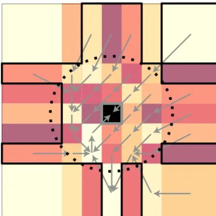
spa-Figure 4. Monte Carlo generation procedure: (i) a spatially
cor-related Gaussian field with an exponential covariance function (mean = 30, partial sill = 8, nugget = 2, range = 3) is generated along
a 7×7 irregular grid. The central pixel (in black) represents
the downstream-most catchment, where runoff is to be predicted. Among the remaining pixels, 24 inner isolated drainage areas (IDA) are within a radius of one spatial correlation range (dashed circle) of the central pixel, and 24 outer pixels are beyond that radius. (ii) A predefined number of inner and outer pixels are randomly selected as part of the set of catchments that are flow-connected to the cen-tral pixel. In the figure, all 24 inner pixels and 12 outer pixels are selected and form the flow catchment outlined with a thick black line. (iii) A tree graph is randomly generated (grey arrows) with its trunk at the prediction pixel and branches passing through all the flow-connected pixels. The random field generated in step one is aggregated along the tree by summing the value of all lower order branches at each confluence. (iv) A new spatially correlated field (mean = 1, partial sill = 0.15, nugget = 0, range = 0.5) is generated at each pixel – that is the observed trend. The trend is multiplied by a predefined trend coefficient (τ=10) and added to the aggregated runoff at each pixel – that is the observed runoff. (v) Based on the observed runoff and (if applicable) trend at the 48 non-central pix-els, TopREML and the compared baseline method (Top-kriging or universal kriging) are used to predict runoff at the central pixel. Pre-diction errors are recorded and the procedure repeated 1000 times to get the mean and variance of the errors.
tially correlated, omitting it in the model specification adds a significant spatially correlated component to the error and Eq. (15) should be used to predict the variance. Conversely, including a trend in the model will cause the remaining error to mostly consists of (spatially uncorrelated) residuals, so in this case Eq. (14) is used.
4 Results 4.1 Case studies
Basin-level predictions of the considered signatures are pre-sented in Fig. 5 for the three cross-validation analyses de-scribed in Sect. 3.1. Figure 5 also provides box plots sum-marizing the distribution of the ensuing cross-validation er-rors. In the three analyses, the prediction errors related to TopREML were comparable to the best alternate method: a linear model for annual specific runoff (Nepal) and Top-kriging for runoff frequency (Nepal) and summer runoff (Austria).
Figure 5a presents results for annual specific runoff in Nepal and shows that observable features play a signif-icant role in the prediction of runoff. The linear model showed a highly significant effect of annual precipitation
(τˆyearlyPrecip(LM) =0.99, t-stat: 9.1) a moderately significant
ef-fect of altitude (τˆ(LM)meanElev=0.39, t-stat: 2.5) and an overall fit ofR2=0.63. The positive sign of the altitude coefficient can be attributed to the effects of glacial melt on runoff, which are more significant at higher altitudes, while the average effect of evapotranspiration explains the negative and noisy inter-cept of−313 mm yr−1. While including rainfall and altitude in the model decreased the median absolute error by 43 % (LM to LM0), further increasing the complexity of the model
by allowing for spatial (UK) and topological effects (TK and TR) did not improve the predictive performance: residuals from the linear regression appeared to be correlated at a range shorter than the distance between the gauges in Nepal. In-deed, fitting the empirical semi-variograms with exponential functions revealed spatial correlation ranges that were on the order of the mean distance between IDA centroids for an-nual streamflow (21.6 km), and significantly below that dis-tance (7.0 km) for the regression residuals. Nonetheless, the lack of parsimony of TopREML did not appear to affect its predictive performance, which almost perfectly reproduced the performance of the linear model – the most parsimonious method.
[image:9.612.62.274.67.279.2]0
500
1500
Annual Specific Runoff in Nepal [mm/y]
LOO A
bs
. Er
ror
TR TK UK LM LM0 0.00 TR TK UK LM0
0.04
0.08
Runoff Frequency in Nepal [d-1]
Summer Streamflow in Austria [m3/s]
0
5
10
15
TR TK UK LM0
(a)
(b)
(c)
0.30 0.35 0.40 0.45 0.50
0.30
0.35
0.40
0.45
0.50
Observed 20 30 40 50 60
20
30
40
50
60
500 1500 2500 3500
500
1500
2500
3500
Observed Observed
[image:10.612.128.470.66.269.2]TopREML Pred.
Figure 5. Results of the comparative cross-validation analyses of (a) specific runoff and (b) wet season runoff frequency in Nepal, and (c)
mean summer streamflow in Austria. First row: box plots with the quartiles and 95 % confidence intervals around the median of leave-one-out (LOO) absolute prediction errors. Compared models are TopREML (TR), Top-kriging (TK), universal kriging (UK), linear regression models
(LM) and the sample mean (LM0). Note that without observable trends (b and c), LM and LM0are equivalent. Second row: catchment level
performance of TopREML. Signatures predicted by TopREML for each catchment in the leave-one-out cross-validation analysis are plotted against the corresponding observed signature. Diagonal lines (x=y) representing perfect fit are also displayed for indicative purposes.
40 60 80 100
0.00
0.02
0.04
0.06
% of basins within range that are connected
RE[UK] - RE[T
R]
0 20 40 60 80 100
0.00
0.02
0.04
0.06
% of basins beyond range that are connected
RE[UK] - RE[T
R]
Ninner= 25% Ninner= 75%
(a)
(b)
(c)
−2
−1
0
1
2
Pr
edic
tion Er
ror
No Trend Trend
TK TR TK TR Obs. mean and std. dev Pred. std. dev
Nouter= 33%
Nouter= 100%
Figure 6. Results of the Monte Carlo experiments. (a) and (b) display the effect of network complexity on the performance of TopREML
relative to universal kriging. Network complexity is given as the ratio of basins beyond (Nouter) and within (Ninner) the spatial correlation
range that are connected – minimum network complexity is modeled when no basins beyond and all basins within the range are flow-connected. Relative performance is computed at each Monte Carlo run as the difference in relative prediction errors between universal kriging and TopREML (i.e., RE[UK] −RE[TR]on (a) and (b)). The graphs display the expectation and standard deviation of that difference over the 1000 Monte Carlo runs. (c) presents the observed (grey boxes) and predicted (black error bars) standard deviation on the prediction errors for Top-kriging (TK) and TopREML (TR). Note that the slight downward biases that appear on the graph remain below 1 % of the expected value of the predicted outcome.
4.2 Numerical simulation
Results from the Monte Carlo analysis are presented in Fig. 6, showing the outcomes of the two numerical experi-ments described in Sect. 3.2.
Figure 6a and b shows the effect of network complexity on the performance of TopREML relative to the baseline perfor-mance of universal kriging. This effect is measured as the dif-ference in the relative errors of the two methods as a function
of Nouter, the ratio of basins beyond the spatial correlation
range of runoff that are flow-connected, andNinner, the ratio
of basins within range that are not flow-connected. The effect is expected to increase withNouterand decrease withNinner,
[image:10.612.127.469.361.475.2]catchments that are located beyond the spatial correlation range, and which are therefore not properly accounted for by universal kriging. Conversely, Fig. 6b shows that the rel-ative performance of TopREML decreases with decreasing network effects within the spatial correlation range. A linear regression of the relative performance of TopREML against
NouterandNinnershowed that both trends are significant and
in the expected direction. However, the positive coefficient associated withNouter (9.1, t-stat: 11.9) is larger in absolute
value and more statistically significant than the negative co-efficient associated with Ninner (−2.6, t-stat: −2.6), which
suggests that the benefits of including distant flow-connected basins outweigh the costs of discarding nearby (but uncon-nected) IDAs.
In Fig. 6c, the Monte Carlo analysis showed that model un-certainty is well predicted by TopREML and strongly under-estimated by Top-kriging, both with and without consider-ing an external trend. Includconsider-ing a trend in the model reduces the prediction variance of TopREML – this effect is expected because the variance explained by the trend is no longer in-cluded in the modeling error. The decrease in the prediction variance is well modeled by TopREML, which predicts the observe model uncertainty almost exactly.
5 Discussion
5.1 Performance of TopREML
Cross-validation outcomes suggest that TopREML is an at-tractive operational tool for predicting streamflow in un-gauged basins. The method performs as well as the best al-ternative approach in the prediction of the considered runoff signatures in Nepal and Austria, and significantly outper-forms Top-kriging in the prediction of modeling uncertain-ties in the numerical analysis. Two distinguishing features of TopREML are responsible for these encouraging results. First, TopREML incorporates the topology of the stream net-work by restricting correlations to runoff observed at flow-connected catchments. This allows TopREML to explicitly model the higher correlation in streamflow anticipated along channels, but comes at the expense of discarding correla-tions with neighboring, but not flow-connected catchments. Such correlations can, for instance, be driven by large-scale weather patterns. This tradeoff was investigated in a Monte Carlo analysis showing that modeling performance increases more rapidly when including distant flow-connected basins (slope in Fig. 6a) than it decreases when discarding nearby unconnected basins (slope in Fig. 6b). Further, empirical cor-relograms of Austrian summer runoff (Fig. 2) reveal signif-icantly lower and shorter-ranged spatial correlations when basins are not flow-connected. Both results suggest that the benefit of accounting for network effects on correlations out-weighs the cost of losing some information on the correla-tion between unconnected basins. Second, the REML
frame-work provides an unbiased estimation of variance parame-ters, even when accounting for observable features. This al-lows TopREML to accurately predict modeling uncertainties even for highly trended and auto-correlated runoff signatures, as visible in the Monte Carlo analysis presented on Fig. 6c. By contrast, the expected downward bias in the kriging es-timation of partial sills (Cressie, 1993) is clearly visible in the underestimation of prediction uncertainties by the Top-kriging method.
TopREML also has considerably lower computational re-quirements than Top-kriging, both in terms of input data and optimization complexity. Unlike Top-kriging, where water-shed polygons are necessary inputs for the regularization procedure, vectors are not fundamentally indispensable for TopREML. Indeed, TopREML does not rely on a distributed point process but assumes homogenous IDAs. It follows that its only fundamental data requirement is a table (i.e., a data.frame) of IDAs displaying the observed regionalization variable and the area, centroid coordinates and network posi-tion (i.e., own ID and downstream ID) of the IDA. When con-sidering runtime, both methods rely on numerical optimiza-tion, but Top-kriging uses it to back calculate the point semi-variogram in its regularization procedure. This may substan-tially increase the dimensionality of the optimization task, depending on the grid resolution chosen for the discretization of the catchment areas, which in turn has a highly significant effect on prediction performances (Skøien et al., 2006). By contrast, the dimensionality of the optimization in TopREML is driven by the number of catchments, not an arbitrary grid. More importantly, TopREML admits a well-defined objec-tive function, the restricted likelihood, that is differentiable if the selected variogram function is differentiable. This allows gradient optimization methods to be used, which are much less computationally intensive than the stochastic algorithm required by Top-kriging. The resampling analysis shown in Appendix C suggests that TopREML reduces the computa-tion runtime by an order of magnitude, relative to the imple-mentation of Top-kriging in the rtop package, for comparable prediction performances.
Figure 7. Global distribution of factors affecting model selection. (a) Spatial repartition of the 8540 stream gauges indexed by the
Global Runoff Data Center (Global Runoff Data Center, 2014).
(b) Dominant rainfall type: orographic rainfall are assumed to
oc-cur in mountains, as defined by the United Nations Environment Programme (WCM, 2000), and have a typical range of 1–10 km (Anders et al., 2006). Convective rainfall are assumed dominant in region with a high frequency of lighting strikes (≥10/km2yr−1) as recorded by the TRMM satellite (LIS, 2011) and have a typ-ical scale of 10–100 km (Bosch et al., 1999; Smith et al., 2005). Frontal precipitations are assumed dominant in the remaining re-gions and have a typical scale in excess of 100 km (Bosch et al., 1999; Xu et al., 2014). (c) Drainage density is estimated based on the Hydro1k data set (Hyd, 2004), using 154 large basins (Wot, 2003) as units of analysis. Drainage densities are displayed in three classes: low (0.01–0.025 km−1), medium (0.025–0.027 km−1) and high (>0.027 km−1).
5.2 Model selection
The regionalization methods assessed in the cross-validation analysis range from simple linear regressions with strong in-dependence assumptions, to complex geostatistical methods that allow for both spatial and topological correlations. Re-sults indicate that while complex methods perform best in general, there seems to be a threshold beyond which increas-ing the complexity of the statistical method does not signif-icantly improve the prediction performance: while a linear
ν
0(D)
D
Density
0 2 4 6 8 10
0.00
0.05
0.10
0.15
0.20
0.25
ν(D)
D
Density
0 2 4 6 8 10
0.00
0.05
0.10
0.15
0.20
0.25
5
1
(a)
(b)
(c)
Figure 8. The probability density functions assumed in Eqs. (A6)
and (A2) represent well the case of adjacent ellipsoidal watersheds illustrated in (a). (b) displays the histogram of distance between two random points within a watershed, overlaid by a plot of Eq. (A6) witha0=3 andaD=1/3. (c) displays the histogram of distance
between one random point on each watershed, overlaid by a plot of Eq. (A2) withac=1/3.
model is better than a simple average for the prediction of annual streamflow in Nepal (Fig. 5a), accounting for spa-tial (UK) and topological (TR) correlation does not further improve predictions. In that situation, parsimony prescribes selecting the least complex of the best performing methods.
Under these conditions, the selection of the optimal method is driven by the interplay between the layout of the gauges and the spatial correlation range of the considered runoff signature. A dense network of flow gauges is neces-sary for geostatistical methods to properly estimate the semi-variogram and improve on predictions from linear regres-sions – the case studies suggest that the mean distance be-tween the gauges must be on the order of half the spatial correlation range of the runoff signature. Sparser gauge den-sities do not allow geostatistical methods to capture spatial correlations and their prediction is effectively driven by the deterministic components of the model, i.e., the intercept and (when available) observable features.
[image:12.612.49.285.69.376.2]be-Input matrices: X, y, A, U, cij
IDAs Input Catchments
Variance components σ2, Φ, ξ
Model parameters τ, u, G
PredicDon yout, Var(yout-‐y)
Output matrices: x, a, Uout, cijout
IDAs Output Catchments
Output parameter g
Differen'al Overlay
Numerical Op'miza'on (Eqn 8.)
Matrix Inversion (Eqns 7 & 10.) GIS
Differen'al Overlay
GIS
(Eqn 7.)
[image:13.612.49.288.63.273.2](Eqns 11-‐14)
Figure 9. Algorithmic chart of the provided TopREML
implemen-tation. Dashed frames and arrows represent vector data and opera-tions and the bold arrow represents the step requiring numerical op-timization. The complexity of the computational tasks represented by the remaining plain arrows is driven by matrix inversion, which is of polynomial complexity. In the figure,Xis a matrix of observed
covariates andy a vector of outcomes measured at the available
gauges, as defined in Eq. (1);x is a vector of identical covariates observed at the prediction location.A,U andcij are matrices of
relative catchment areas, network topology and inter-centroidal dis-tances of the available gauges, as defined in Eq. (6);a,Uoutand cijoutare equivalent matrices for the prediction location.σ2,φandξ are estimated variance parameters as defined in Eq. (3);τ,uandG are the estimated fixed and random effects (Eq. 11) and variance– covariance matrix (Eq. 7);gis the estimated covariance at the pre-diction location (used in Eq. 13). Finally,youtand Var(yout−y)are
the predicted outcome and the related prediction variance.
low the mean distance between the gauges (13.9 km). In that case there is a tradeoff between relying on observable fea-tures or variance information to make a prediction, and par-simony and stationarity considerations come into play when selecting the regionalization model. For instance, while par-simony generally prescribes the use of observable features, a climate may be less stationary – and therefore a less reliable external trend – than embedded geology or geomorphology.
In general, geostatistical approaches improve on the pre-diction of ungauged basins if the distance between the stream gauges is significantly smaller than the spatial correlation scale of runoff. Favorable areas are characterized by high drainage densities or localized rainfall, in addition to a high density of streamflow gauges. All three variables are highly heterogeneously distributed at a global scale, as seen on Fig. 7. The multiplicity of local settings likely explains the large diversity of existing regionalization methods and sug-gests that the selection of the optimal regionalization ap-proach has to be made locally.
20 30 40 50
N gauges
Relati
ve Error
Ratio
Runtime Ratio
Spherical Exponential
0.1
1.0
10
0.1
1.0
10
Figure 10. Leave-one-out cross-validation results for Austrian
sum-mer flow when resampling a subset of the training gauges. Compu-tational performances are represented as the ratio of runtimes for TopREML against Top-kriging. Prediction performances are rep-resented as the ratio of relative errors. TopREML performances when using gradient-based and stochastic optimization algorithms are represented as circles and triangles, respectively. Points repre-sent the median value and error bars reprerepre-sent 90 % confidence in-tervals over 200 repetitions.
Lastly, the decreasing returns to improvements in the com-plexity of the model also suggest that the performance of sta-tistical methods for PUB is ultimately bounded by the spa-tial heterogeneity of runoff generating processes. Statistical methods resolve parts of that heterogeneity using the spatial distribution of observable features (linear regressions) and/or based on the analysis of the variance of a sample of the pre-dicted variable (geostatistics). Yet very important parts of the hydrological activity related to storage and flow path char-acteristics take place underground: they cannot be observed and included in the statistical models (Gupta et al., 2013). This residual spatial heterogeneity can ultimately only be re-solved through a better understanding of the particular catch-ment processes governing runoff in the considered region. Approaches coupling statistical regionalization with process-based models that assimilate both a conceptual understand-ing of catchment-scale processes and the random nature of runoff (e.g., Botter et al., 2007; Schaefli et al., 2013; Müller et al., 2014) are particularly promising.
6 Conclusions
[image:13.612.330.520.65.211.2]The method was successfully tested in cross-validation analyses on mass conserving (mean streamflow) and non-conservative (runoff frequency) runoff signatures in Nepal (sparsely gauged) and Austria (densely gauged), where it matched the performance of the best alternative method: Top-kriging in Austria and linear regression in Nepal. TopREML outperformed Top-kriging in the prediction of uncertainty in Monte Carlo simulations and its performance is robust to the inclusion of observable features.
Appendix A: Covariance of a spatially averaged process The aim of this analysis is to explore the likely forms of a correlation structure between spatially aggregated processes, given that the underlying point-scale processes are also spa-tially correlated. In order to maintain tractability, the analy-sis will consider a strongly idealized case. While we antic-ipate deviations from the results in non-ideal situations, we nonetheless interpret this idealized analysis as offering in-sight that constrains the choice of correlation function in the TopREML analysis.
Assuming that the underlying point-scale processYis con-servative, the aggregated processyk0 related to the subcatch-mentSkof gaugekcan be expressed as
yk0 = 1
Ak
Z
Sk
Y (x)dx,
whereAkis the area ofSk.
To proceed, we make the assumption that the area of the drainage areas Sk are approximately equal. While this
is a strong constraint, under situations where gauges are placed near confluences and where subcatchments for a given stream ratio are adequately monitored by the gauge network, Horton scaling ensures that the drainage areas are of a similar order of magnitude. Thus, we will takeAk=A∀k. The
sub-catchments are further assumed to have similar shapes and (by definition) do not overlap.
Following Cressie (1993) (p. 68), the covariance between two aggregated random variablesyk0 andy0mis expressed as a function of the covariogramCP(·)of the underlying
point-scale process: Cov yk0, ym0= 1
A2
Z
Sk
Z
Sm
CP(|x2−x1|)dx1dx2
=
∞ Z
0
ν(D)CP(D)dD, (A1)
where Sk andSm are the surfaces of subcatchments k and
m, andν(D)is the probability density function of the dis-tance between randomly chosen points within Sk andSm–
two identical and non-overlapping shapes. Analytical expres-sions for ν(D)can be derived for simple geometries (e.g., Mathai, 1999), although complex algebraic expressions typ-ically result. For analytical tractability we adopt a simplified expression:
ν(D)=
(
a0exp (−aDD+acc) ifc−D1≤D≤c+D2
0 otherwise,
(A2) which approximates distance frequency function of adjacent elliptical subcatchments, as shown in Fig. 8. In Eq. (A2) the
parametersa0,aD> ac,D1andD2are positive functions of
A, andc is the distance between the centroids of the sub-catchments.
We also assume that the underlying point-scale process is second-order stationary and follows an exponential correla-tion funccorrela-tion:
CP(D)=σp2exp −apD, (A3)
whereσp2andapare respectively the point variance and
spa-tial range of the process.
Inserting Eqs. (A2) and (A3) into Eq. (A1) allows the co-variance of the two spatially aggregated random variables to also be expressed as an exponential function of the distance cbetween their supports
CA(c)=ξ σ2exp(−φc) , (A4)
where ξ σ2= σ
2 pa0
ap+aD [exp(apD2+aDD2) – exp(−apD1− aDD1)]>0 andφ=ap+aD−ac>0. This exponential form
was adopted in the covariance derivation in the main text. We note that within this analysis, the spatial aggregation of the point-scale process creates a nugget variance arising from spatial correlation scales smaller than the subcatch-ments. The nugget variance can be derived (for this idealized case) by considering the average covariance of points within the catchments:
Cov y0k, yk0= 1
A2
Z
Sk
Z
Sk
CP(|x2−x1|)dx1dx2
=
∞ Z
0
ν0(D)CP(D)dD, (A5)
whereν0(D)now represents the probability density function
(pdf) of the distance between two randomly selected points withinSk:
ν(D)=
(
a0exp(−aDD) if 0≤D≤D0
0 otherwise, (A6)
where D0 is the maximum distance between two points
withinSk. Again, inserting Eqs. (A6) and (A3) into Eq. (A5),
we get the nugget variance resulting from spatial aggrega-tion:
CA,0=
σp2a0
ap+aD
1−exp(−apD0−aDD0)
. (A7)
Therefore, under the aforementioned assumptions, catchment-scale variance parametersσ2andξ in Eq. (6) can be expressed in terms of point-scale parameters:
σ2= σ 2
pa0
ap+aD
1−exp(−apD0−aDD0). (A8)
ξ=exp(apD2+aDD2)−exp(−apD1−aDD1)
1−exp(−apD0−aDD0)
Appendix B: Propagation of runoff frequency in a stream network
We describe runoff occurrence as a binary random variable taking the value of 1 if an increase in daily streamflow occurs and 0 otherwise. If runoff events are uncorrelated in time, the random variable follows a Bernouilli distribution with fre-quencyλ. At a given gauge on a given day, the random vari-able takes a value of 0 if all of the upstream gauges take a value of 0.
In a simple situation with two upstream sub-basins de-scribed by the random variablesXandY, the frequencyPZ
of the random variableZ=max(X, Y )can be described as 1−PZ=P!X,!Y =P!XP!Y|!X=P!X(1−PY|!X)
=(1−PX)(1−PY|!X),
where!X stands for the eventX=0. Applying the law of total probabilities to substitutePY|!Xgives
1−PZ=(1−PX)
1−PY−PXPY|X
1−PX
.
The covariance ofXandY can be derived as CovX, Y =EXY−EXEY =PXPY|X−PXPY
with EXY=0·P!X,!Y+0·P!X,Y+0·PX,!Y+1·PX,Y=
PXPY|X. Finally, substituting PXPY|X for the covariance
expression, yields: 1−PZ=(1−PX)
1−PY−[CovX, Y+PXPY]
1−PX
=(1−PX)(1−PY)+CovX, Y.
Extending the above derivation to multiple sub-basins and neglecting the covariance term leads to a linear relation be-tween runoff frequencies at gaugeiand at upstream gauges in the following form:
ln(1−λi)≈
k∈UPi
X
k=i
ln(1−λk). (B1)
Thus, if runoff pulses occur independently for each sub-basin, TopREML can be applied to ln(1−λ)(settingak=1),
to estimate runoff frequency at ungauged sites.
Appendix C: Computational performance of TopREML An algorithmic chart of TopREML, as implemented in the provided script, is presented in Fig. 9. IDAs and the topology of the stream network are extracted from the nested catch-ment using differential overlay. TopREML uses the BFGS algorithm (Wright and Nocedal, 1999) to maximize the re-stricted likelihood, with the option of using a stochastic op-timization algorithm (Simulated Annealing, Belisle, 1992) if a non-differentiable (e.g., spherical) covariance function is selected.
The Supplement related to this article is available online at doi:10.5194/hess-19-2925-2015-supplement.
Acknowledgements. The authors would like to thank Michèle
Müller, Morgan Levy, David Dralle, Gabrielle Boisramé and two anonymous reviewers for their helpful review and comments. Data have been graciously provided by the Department of Hydrology and Meteorology of Nepal, the HKH-FRIEND project and the rtop package. The Swiss National Science Foundation are gratefully acknowledged for funding (M. F. Müller). Publication made possible in part by support from the Berkeley Research Impact Initative (BRII) sponsored by the UC Berkeley Library.
Edited by: J. Freer
References
Anders, A. M., Roe, G. H., Hallet, B., Montgomery, D. R., Finnegan, N. J., and Putkonen, J.: Spatial patterns of precipita-tion and topography in the Himalaya, Geol. Soc. Am. Special Papers, 398, 39–53, 2006.
Bishop, G. D. and Church, M. R.: Automated approaches for re-gional runoff mapping in the northeastern United States, J. Hy-drol., 138, 361–383, 1992.
Belisle, C. J. P.: Convergence theorems for a class of simulated an-nealing algorithms on Rd, J. Appl. Probab., 29, 885–895, 1992. Blöschl, G., Sivapalan, M., Wagener, T., Viglione, A., and Savenije,
H.: Runoff prediction in ungauged basins: Synthesis across pro-cesses, places and scales, Cambridge University Press, 2013. Bosch, D., Sheridan, J., and Davis, F.: Rainfall characteristics and
spatial correlation for the Georgia Coastal Plain, Trans. ASAE, 42, 1637–1644, 1999.
Botter, G., Porporato, A., Rodriguez-Iturbe, I., and Rinaldo, A.: Basin-scale soil moisture dynamics and the probabilistic char-acterization of carrier hydrologic flows: Slow, leaching-prone components of the hydrologic response, Water Resour. Res., 43, W02417, doi:10.1029/2006WR005043, 2007.
Castiglioni, S., Castellarin, A., Montanari, A., Skøien, J. O., Laaha, G., and Blöschl, G.: Smooth regional estimation of low-flow in-dices: physiographical space based interpolation and top-kriging, Hydrol. Earth Syst. Sci., 15, 715–727, doi:10.5194/hess-15-715-2011, 2011.
Chalise, S., Kansakar, S., Rees, G., Croker, K., and Zaidman, M.: Management of water resources and low flow estimation for the Himalayan basins of Nepal, J. Hydrol., 282, 25–35, 2003. Corbeil, R. R. and Searle, S. R.: Restricted maximum likelihood
(REML) estimation of variance components in the mixed model, Technometrics, 18, 31–38, 1976.
Cressie, N.: Statistics for Spatial Data, Wiley, New York, NY, 1993. Cressie, N., Frey, J., Harch, B., and Smith, M.: Spatial prediction on a river network, J. Agr. Biol. Environ. Stat., 11, 127–150, 2006. Department of Hydrology and Meteorology: Daily Streamflow and
Precipitation Data, Kathmandu, 2011.
D’Odorico, P. and Rigon, R.: Hillslope and channel contribu-tions to the hydrologic response, Water Resour. Res., 39, 1113, doi:10.1029/2002WR001708, 2003.
Gilmour, A., Thompson, R., and Cullis, B.: Average Information REML: an efficient algorithm for variance parameter estimation in linear mixed models, Biometrics, 51, 1440–1450, 1995. Gilmour, A., Cullis, B., Welham, S., Gogel, B., and Thompson, R.:
An efficient computing strategy for prediction in mixed linear models, Comput. Stat. Data Anal., 44, 571–586, 2004.
Global Runoff Data Center: Global Runoff Data Base, Global Runoff Data Centre. Koblenz, Federal Institute of Hydrology (BfG), 2014.
Goovaerts, P.: Geostatistics in soil science: state-of-the-art and per-spectives, Geoderma, 89, 1–45, 1999.
Goovaerts, P.: Geostatistical approaches for incorporating elevation into the spatial interpolation of rainfall, J. Hydrol., 228, 113–129, 2000.
Gottschalk, L.: Interpolation of runoff applying objective methods, Stoch. Hydrol. Hydraul., 7, 269–281, 1993.
Gottschalk, L., Krasovskaia, I., Leblois, E., and Sauquet, E.: Map-ping mean and variance of runoff in a river basin, Hydrol. Earth Syst. Sci., 10, 469–484, doi:10.5194/hess-10-469-2006, 2006. Gupta, H., Blöschl, G., McDonnell, J., Savenije, H., Sivapalan,
M., Viglione, A., and Wagener, T.: Outcomes of Synthesis, in: Runoff Prediction in Ungauged Basins: Synthesis across Pro-cesses, Places and Scales, edited by: Blöschl, G., Sivapalan, M., Wagener, T., Viglione, A., and Savenije, H., Cambridge Univer-sity Press, 2013.
Henderson, C. R.: Best linear unbiased estimation and prediction under a selection model, Biometrics, 31, 423–447, 1975. Huang, W.-C. and Yang, F.-T.: Streamflow estimation using
Krig-ing, Water Resour. Res., 34, 1599–1608, 1998.
HYDRO1k Elevation Derivative Database, U.S. Geological Survey Earth Resources Observation and Science (EROS) Center, Sioux Falls, South Dakota, 2004.
Laaha, G., Skøien, J. O., Nobilis, F., and Blöschl, G.: Spatial predic-tion of stream temperatures using Top-kriging with an external drift, Environ. Modell. Assessm., 18, 671–683, 2013.
Laaha, G., Skøien, J., and Blöschl, G.: Spatial prediction on river networks: comparison of Top-kriging with regional regression, Hydrol. Process., 28, 315–324, 2014.
Lark, R., Cullis, B., and Welham, S.: On spatial prediction of soil properties in the presence of a spatial trend: the empirical best linear unbiased predictor (E-BLUP) with REML, Eur. J. Soil Sci., 57, 787–799, 2006.
LIS Global lightning Image, NASA EOSDIS Global Hydrology Re-source Center (GHRC) DAAC, Huntsville, AL, 2011.
Mathai, A. M.: An introduction to geometrical probability: distribu-tional aspects with applications, Vol. 1, CRC Press, Boca Raton, FL, 1999.
Merz, R. and Blöschl, G.: Flood frequency regionalisation – spa-tial proximity vs. catchment attributes, J. Hydrol., 302, 283–306, 2005.
Müller, M. F. and Thompson, S. E.: Bias adjustment of satellite rain-fall data through stochastic modeling: Methods development and application to Nepal, Adv. Water Resour., 60, 121–134, 2013. Müller, M. F., Dralle, D. N., and Thompson, S. E.: Analytical model
for flow duration curves in seasonally dry climates, Water Re-sour. Res., 50, 5510–5531, 2014.
Olea, R.: Optimal contour mapping using universal kriging, J. Geo-phys. Res., 79, 695–702, 1974.
Patterson, H. D. and Thompson, R.: Recovery of inter-block infor-mation when block sizes are unequal, Biometrika, 58, 545–554, 1971.
Pebesma, E. J.: Multivariable geostatistics in S: the gstat package, Comput. Geosci., 30, 683–691, 2004.
R Core Team: R: A language and environment for statistical com-puting, R Foundation Statistical Comcom-puting, 2008.
Sauquet, E.: Mapping mean annual river discharges: geostatistical developments for incorporating river network dependencies, J. Hydrol., 331, 300–314, 2006.
Sauquet, E., Gottschalk, L., and Leblois, E.: Mapping average an-nual runoff: a hierarchical approach applying a stochastic inter-polation scheme, Hydrol. Sci. J., 45, 799–815, 2000.
Schaefli, B., Rinaldo, A., and Botter, G.: Analytic probability distri-butions for snow-dominated streamflow, Water Resour. Res., 49, 2701–2713, 2013.
Sivapalan, M., Konar, M., Srinivasan, V., Chhatre, A., Wutich, A., Scott, C., Wescoat, J., and Rodríguez-Iturbe, I.: Socio-hydrology: Use-inspired water sustainability science for the Anthropocene, Earth’s Future, 2, 225–230, 2014.
Skøien, J. O., Merz, R., and Blöschl, G.: Top-kriging – geostatis-tics on stream networks, Hydrol. Earth Syst. Sci., 10, 277–287, doi:10.5194/hess-10-277-2006, 2006.
Skøien, J., Blöschl, G., Laaha, G., Pebesma, E., Parajka, J. and Viglione, A.: rtop: An R package for interpolation of data with a variable spatial support, with an example from river networks, Comput. Geosci., 67, 180–190, 2014.
Smith, D. F., Gasiewski, A. J., Jackson, D. L., and Wick, G. A.: Spatial scales of tropical precipitation inferred from TRMM mi-crowave imager data, Geoscience and Remote Sensing, IEEE Trans., 43, 1542–1551, 2005.
Srinivasan, V., Thompson, S., Madhyastha, K., Penny, G., Jeremiah, K., and Lele, S.: Why is the Arkavathy River drying? A multiple-hypothesis approach in a data-scarce region, Hydrol. Earth Syst. Sci., 19, 1905–1917, doi:10.5194/hess-19-1905-2015, 2015. Stokstad, E.: Scarcity of rain, stream gages threatens forecasts,
Sci-ence, 285, 1199–1200, 1999.
Ver Hoef, J. M. and Peterson, E. E.: A moving average approach for spatial statistical models of stream networks, J. Am. Stat. Assoc., 105, 6–18, 2010.
Ver Hoef, J. M., Peterson, E., and Theobald, D.: Spatial statistical models that use flow and stream distance, Environ. Ecol. Stat., 13, 449–464, 2006.
Viglione, A., Parajka, J., Rogger, M., Salinas, J. L., Laaha, G., Siva-palan, M., and Blöschl, G.: Comparative assessment of predic-tions in ungauged basins – Part 3: Runoff signatures in Austria, Hydrol. Earth Syst. Sci., 17, 2263–2279, doi:10.5194/hess-17-2263-2013, 2013.
Watersheds of the World, IUCN, IWMI, Rasmar Convention Bu-reau and WRI World Resources Institute, Washington, DC, 2003. Wittenberg, H. and Sivapalan, M.: Watershed groundwater balance estimation using streamflow recession analysis and baseflow sep-aration, J. Hydrol., 219, 20–33, 1999.
World Conservation Monitoring Centre (UNEP-WCMC): Moun-tains and Forests in MounMoun-tains, UNEP-WCMC, Cambridge, 2000.
Wright, S. and Nocedal, J.: Numerical optimization, Vol. 2, Springer New York, NY, 1999.