www.hydrol-earth-syst-sci.net/19/3585/2015/ doi:10.5194/hess-19-3585-2015
© Author(s) 2015. CC Attribution 3.0 License.
Stochastic approach to analyzing the uncertainties
and possible changes in the availability of water
in the future based on scenarios of climate change
G. G. Oliveira, O. C. Pedrollo, and N. M. R. Castro
Institute of Hydraulic Research – Federal University of Rio Grande do Sul, Porto Alegre, RS, Brasil
Correspondence to: G. G. Oliveira (g.g.oliveira10@gmail.com)
Received: 11 December 2014 – Published in Hydrol. Earth Syst. Sci. Discuss.: 10 April 2015 Accepted: 3 August 2015 – Published: 17 August 2015
Abstract. The objective of this study was to analyze the changes and uncertainties related to water availability in the future (for the purposes of this study, the period be-tween 2011 and 2040 was adopted), using a stochastic ap-proach, taking as reference a climate projection from cli-mate model Eta CPTEC/HadCM3. The study was applied to the Ijuí River basin in the south of Brazil. The set of methods adopted involved, among others, correcting the cli-matic variables projected for the future, hydrological sim-ulation using artificial neural networks (ANNs) to define a number of monthly flows and stochastic modeling to gen-erate 1000 hydrological series with equal probability of oc-currence. A multiplicative type stochastic model was devel-oped in which monthly flow is the result of the product of four components: (i) long-term trend component; (ii) cyclic or seasonal component; (iii) time-dependency component; and (iv) random component. In general, the results showed a trend to increased flows. The mean flow for a long pe-riod, for instance, presented an alteration from 141.6 m3s−1 (1961–1990) to 200.3 m3s−1(2011–2040). An increment in mean flow and in the monthly standard deviation was also observed between the months of January and October. Be-tween the months of February and June, the percentage of mean monthly flow increase was more marked, surpassing the 100 % index. Considering the confidence intervals in the flow estimates for the future, it can be concluded that there is a tendency to increase the hydrological variability during the period between 2011 and 2040, which indicates the possibil-ity of occurrence of time series with more marked periods of droughts and floods.
1 Introduction
Discussions concerning variability and climate changes have intensified in the last few decades. Many studies have proved significant alterations in the composition of the at-mosphere and in the concentration of gases that have im-plications for thermal energy, changing climate-related vari-ables. On this topic the Intergovernmental Panel on Climate Change (IPCC) should be highlighted.
The IPCC was established in 1988 by the World Meteo-rological Organization (WMO) and by the United Nations Environment Program (UNEP). The objective is to supply scientific information in order to gain a better understanding of changes in the global climate, so as to evaluate their im-pact on society and on nature, and propose alternatives for adaptation and mitigation.
According to the IPCC (2013), it is already clear that the Earth has been warming since the beginning of the industrial period, as proved by the rise in the mean temperatures of the air and the oceans. Consequently, negative impacts have been observed as the increase in the mean level of the seas and the acceleration of ice melt in mountain or polar climate regions. Studies developed on a global scale have shown that several natural systems are already under the impact of cli-mate changes.
growth, increasing the risk of losses in harvests worldwide (Mearns et al., 1996; Richter and Semenov, 2005; Zhang and Liu, 2005; Rasmussen et al., 2012).
The climate scenario projections are performed using global climate models (GCMs) and regional climate mod-els (RCMs). The resolution of RCMs is between 10 and 50 km, which allows one to apply them in scenarios of cli-mate changes in medium and small basins. Using these mod-els, together with the GCMs, enables detailing of the cli-mate processes at the local level, detecting the variations and specificities of a given region and thus improving the under-standing of impacts in small basins (Marengo et al., 2009, 2012).
The Eta model was developed at Belgrade University and operationally implemented by the National Centers for En-vironmental Prediction (Black, 1994). The vertical coordi-nate system used in this model is recommended for use over South America due to the presence of the Andes mountain range (Marengo et al., 2012). Recently, a new version of the Eta model, Eta CPTEC, was developed independently by the National Institute for Space Research (INPE).
The regional Eta model was configured over South Amer-ica and applied to downscale HadCM3 members of the Per-turbed Physics Ensemble (PPE) experiment for the baseline (1961–1990). The dynamic downscaling method was used to generate the climate scenarios (Chou et al., 2012). According to Mujumdar and Kumar (2013), the main advantage of dy-namical downscaling over the statistical downscale method is its ability to capture the mesoscale nonlinear effects. Fur-thermore, the dynamical downscaling provides information for many climate variables while ensuring internal consis-tency with respect to the physical principles in meteorology, simulating satisfactorily some regional climatic conditions.
The Eta CPTEC model includes the increase in CO2 con-centration levels according to the scenario of emission and daily variation of the state of vegetation during the year. This model reproduces scenario A1B of IPCC SRES, supplied by the global coupled ocean–atmosphere HadCM3, in four members (versions) of disturbance in the global model (no disturbance – CNTRL; low sensitivity – LOW; medium sen-sitivity – MID; high sensen-sitivity – HIGH), which represent the uncertainty of boundary conditions, to produce variants of the same model (Chou et al., 2012; Marengo et al., 2012). The regional model was integrated into the horizontal reso-lution of 40 km, for the period between 1961 and 1990, and the future scenarios were generated in three 30-year periods (from 2011 to 2040, from 2041 to 2070, and from 2071 to 2100) (Chou et al., 2012).
The study of Marengo et al. (2012) details the scenarios generated for South America using the Eta CPTEC/HadCM3 model. According to this study, the model is configured with 38 vertical layers, with the top of the model at 25 hPa. The Mellor–Yamada level 2.5 procedure (Mellor and Ya-mada, 1974) was used for the treatment of turbulence. The radiation package was developed by the Geophysical
Fluid Dynamics Laboratory, based on studies by Fels and Schwarzkopf (1975) and Lacis and Hansen (1974). The Eta model uses the Betts–Miller (Betts and Miller, 1986) scheme modified by Janjic (1994) to parameterize deep and shallow cumulus convection and the Zhao scheme (Zhao et al., 1997) to parameterize cloud microphysics. This model also uses the NOAH scheme (Ek et al., 2003) to parameterize the land-surface transfer processes (Marengo et al., 2012).
Pesquero (2009), Chou et al. (2012) and Marengo et al. (2012) used model Eta CPTEC. In the first two studies, the model was used to reproduce the present climate in South America and to certify the quality of the model. A smooth tendency was observed to underestimate precipitation over the Amazon in the rainy season and the central region of Brazil, in the Brazilian savanna. In the last study (Marengo et al., 2012), model Eta CPTEC was used to study the cli-mate changes in the Amazon, São Francisco and Paraná river basins between 2011 and 2100.
Currently, in the scientific literature, there are several stud-ies that analyze the effects of climate changes on water avail-ability (e.g., Kleinn et al., 2005; Hughes et al., 2011; Gu-nawardhana and Kazama, 2012). On a continental or global scale, normally, the outputs of the GCMs are used in com-bination with the empirical macroscale hydrological models that perform the water balance (for instance, Arnell, 1999, 2004; Nijssen et al., 2001; Milly et al., 2005; Nohara et al., 2006). The studies on water availability in smaller river basins normally use the climate projections for the RCMs, associated with empirical or physically based hydrological models, in a deterministic approach, offering only a single result in the hydrological sphere for each climate scenario. Examples of this are the studies by Middelkoop et al. (2001), Menzel and Bürger (2002) and Kleinn et al. (2005).
However, because of the randomness of hydrometeorolog-ical processes, the uncertainties related to climate modeling and future water availability favor the use of probabilistic methods based on stochastic time series, as in the studies by Wilks (1992), Semenov and Barrow (1997) and Booij (2005). The stochastic approach broadens the possibility of analyz-ing water availability and the climatic uncertainties in the fu-ture, offering a great number of scenarios for analysis. Thus, it is possible to identify the confidence intervals in the pro-jection and to estimate the random component of the climatic and hydrological dynamics.
However, when generating hundreds or thousands of stochastic climate series, it is necessary to repeat the hydro-logical simulation often, rendering the modeling process very onerous from the computational standpoint. Moreover, in this approach the hydrological scenarios produced become even more sensitive to any imprecision in estimating the parame-ters of the rainfall-flow transformation model.
Figure 1. Location of the Ijuí River basin, section upstream from the Santo Ângelo gauging station (5414 km2), RS, Brazil.
climate scenario, a flow series is generated by hydrological deterministic simulation and then the stochastic process is performed.
The objective of this study is to analyze the possible sce-narios and uncertainties related to water availability in future, using a stochastic approach based on a climatic change sce-nario originating in the Eta CPTEC/HadCM3 climate model. This study will be applied to the Ijuí River basin, in Rio Grande do Sul (RS), Brazil.
2 Methodology
The set of methods adopted in this study comprised the use of observed and simulated hydrometeorological data to analyze the uncertainties and possible scenarios of water availability in the future, based on scenario A1B of IPCC SRES, gener-ated by regional climate model Eta CPTEC/HadCM3.
First, it is important to emphasize that the selection of the climate change scenario was made at the beginning of a research project (2010–2014). At that time, the new IPCC scenarios, for the AR5, were not yet available. Furthermore, all the data from climate model Eta CPTEC were provided by the National Institute for Space Research (INPE). This agency has recommended the use of the A1B scenario in four versions with different sensitivities. These versions were al-ready being examined in large areas of the South American continent (e.g., Marengo et al., 2012). Therefore, given this context, the impacts of climate changes in medium and small river basins of Brazil were evaluated in more detail with the use of the A1B scenario.
For this study, considering the availability of the cli-matic data derived from regional climate model Eta CPTEC/HadCM3, the years between 1961 and 1990 were considered as the “base” period, and the years between 2011 and 2040 as the “future” period.
Simplifying, the methodological procedure covered (i) spatial interpolation of the meteorological variables; (ii) selection of the climatic scenario and correction of the climate variables; (iii) estimation of the potential evapotran-spiration; (iv) hydrological simulation using artificial neural networks (ANNs); and (v) stochastic modeling of monthly flows to generate possible hydrological series in the future. 2.1 Study area
This study was applied in the Ijuí River basin, in the Santo Ângelo stream gauging section, in the northwest of RS, Brazil. The basin area is 5414 km2and it is located between the following geographic coordinates: latitudes 27.98 to 28.74◦S and longitudes 53.21 to 54.28◦W (Fig. 1). At this stream gauging station between 1941 and 2005, the mean flow (Q) was 138 m3s−1, and the dry and high flow peri-ods were the months of March (Q=72 m3s−1) and October (Q=211 m3s−1), respectively.
Considering the daily weather observations of the Cruz Alta station, operated by INMET (National Institute of Me-teorology), the winter and spring months (from June to De-cember) are the rainiest. According to Rossato (2011), the annual rainfall is 1750 mm, which occurs within 110 days during the year. The annual mean temperature oscillates be-tween 17 and 20◦C. The coldest months are June and July, with a mean of around 14◦C, and the warmest months are January and February, with a mean of around 24◦C. 2.2 Data
The following materials were used in this study:
i. daily historical series of precipitations provided by the HidroWeb site of the National Water Agency (ANA), during the period between 1961 and 1990, at 77 rain gauging stations within the radius of coverage of 100 km of the basin boundaries (Fig. 2);
ii. daily historical series of precipitation provided by IPH (Castro et al., 1999), in the years 1989 and 1990, at 22 rain gauging stations (Fig. 2);
iii. daily historical series of precipitation, temperature, wind speed, solar radiation, atmospheric pressure and relative humidity of the air provided through the por-tal of BDMEP (Bank of Meteorological Data for Teach-ing and Research) of INMET, durTeach-ing the period between 1961 and 1990, at five meteorological stations (Fig. 2); iv. daily historical series of flows from the Santo Ângelo
station, located at coordinates 28.36◦S and 54.27◦W, provided through the HidroWeb site, during the period between 1961 and 1990;
v. daily data simulated by regional climate model Eta CPTEC, conducted by four members of global cli-mate model HadCM3, with different levels of sensitiv-ity (CNTRL, LOW, MID and HIGH), during the peri-ods of 1961–1990 (“base”) and 2011–2040 (“future”). The variables simulated were precipitation, tempera-ture, wind speed, relative humidity of the air, atmo-spheric pressure and solar radiation.
2.3 Spatial interpolation
[image:4.612.311.547.66.302.2]The first stage consisted of the spatial interpolation of the five daily climate variables (temperature, wind speed, relative hu-midity of the air, atmospheric pressure and solar radiation) and daily precipitation in the periods between 1961–1990 (observed and simulated data) and 2011–2040 (data simu-lated by the Eta model). The interpolation grid was generated with a spatial resolution of 5 km (Fig. 2), totalizing 264 nodes in the basin area. The interpolation procedure was performed for all data sets: (i) series observed at 104 rain gauging or meteorological stations; and (ii) series simulated using model
Figure 2. Location of the stations with hydrologic and climate data
used in a radius of coverage of 100 km in relation to the Ijuí River basin.
Eta CPTEC/HadCM3 in four scenarios of climate sensitivity (CNTRL, LOW, MID and HIGH).
The use of so many stations in a 100 km radius to begin the interpolation process consists of a safety margin, since many of these stations present short series, with many gaps. Thus, only on a few days when the stations closest to the in-terpolation grid present gaps, the method can select rainfall data from stations located slightly further away, in this way avoiding failures in estimating precipitation during the inter-polation process. It can be said that for each day, in every node of the interpolation grid, only the closest stations with rainfall data were used, usually within the basin and imme-diate surroundings.
The interpolation method used was that of the natural neighbor (Sibson, 1981). This interpolation method obtained the best results in the study presented by Silva et al. (2013), with precipitation series similar to those used in the present study, also in the Ijuí River basin. In the study mentioned, the following methods were also tested: closest neighbor, linear triangulation and inverse distance weighting.
Still at this stage, the daily mean value of the five climate variables and of precipitation in the Ijuí River basin was cal-culated, considering the data observed and the data simulated by the ETA model. Finally, the monthly accumulated precip-itation for the observed series and for scenarios simulated by the Eta model in the periods of 1961–1990 (base) and 2011– 2040 (future) were calculated.
2.4 Selection of climate scenario and correction of climate variables
The outputs of climate models should not be used directly to estimate future water availability (Graham, 2000). The cli-mate models may not represent perfectly the current clicli-mate due mainly to the influence of the spatial discretization of the models. It is observed (Lenderink et al., 2007) that the out-puts may present systematic errors. The correction of climate variables is intended to prevent the errors intrinsic to the out-put of the climate models being propagated to the subsequent hydrologic modeling.
Recently several techniques to correct the climate vari-ables resulting from the GCMs and RCMs were developed and compared (Themeßl et al., 2012). The use of distur-bances (Delta change approach) in climate variables is a commonly used strategy to simulate the impacts of climate changes, obtained via global or regional climate models of water resources (Graham, 2004; Lenderink et al., 2007). The technique consists of using only the seasonal change fore-seen between the current and future scenario, obtained with the climate model. This change is represented by the differ-ence between the current climatic conditions and those fore-seen for the future, both conditions obtained by the climate model. The change foreseen is incorporated into the histor-ical series of precipitations and temperature to generate the series in the future. Thus the error associated with climate modeling is eliminated from the current conditions, and be-comes limited to the uncertainties associated with the fore-cast of climate changes for the future. Examples of applying this methodology are the studies by Kaczmarek et al. (1996), Lettenmaier et al. (1999), Graham (2000) and Bergström et al. (2001).
However, as mentioned by the authors themselves (Gra-ham, 2000; Bergström et al., 2001), and supported by Lenderink et al. (2007), applying the forecast changes in tem-perature or in precipitation directly to the series observed im-plies considerable simplifications that may compromise the analysis of the projections in future. In this approach, for in-stance, probable changes in the number of rainy days, in dis-persion (variance) of rains or in the extreme values of tem-perature are not considered. This occurs because the series itself observed in the past consists of the base of forecasts for the future, and only the seasonal mean variations are taken into account. In this case, there is a risk of considering that the same anomalies recorded in the past will be observed in
the future with small changes in the monthly magnitude of climate variables, according to time of the year.
Thus, Lenderink et al. (2007) discuss and analyze how the output of a regional climate model should be corrected to obtain more realistic flows for the current climate and, con-sequently, for the future climate. According to the authors, the development of a regional climate model, with some cor-rections in the output, allows the direct approach in using projections of temperature and rainfall for the future. This method, instead of adding the changes forecast in the series observed, performs a different procedure: (i) it detects the differences between the current climatic conditions, i.e., be-tween the conditions observed using meteorological stations and the conditions simulated by the regional climate model; and (ii) it applies these differences in the series forecast for the future.
Other more sophisticated methods have been tested and compared, with applications at daily or monthly time in-tervals, as can be seen in Wood et al. (2004), Maurer and Hidalgo (2008), Boé et al. (2007), Piani et al. (2010) and Bárdossy and Pegram (2011). In a recent study, Themeßl et al. (2011) compared a few correction methods and con-cluded that the quantile-based mapping technique (Panofsky and Brier, 1968) is the most effective one to remove the er-rors in the precipitation data. This method is applied with small adaptations in the studies listed above. Essentially, the method is based on the differences between the accumu-lated probability curves (simuaccumu-lated and observed) of daily or monthly precipitations.
In the study by Oliveira et al. (2015a), whose objective was to evaluate the climatic conditions simulated using model Eta CPTEC/HadCM3, emphasizing the study of water availabil-ity in the Ijuí River basin, four methods to correct the cli-mate variables were tested: (i) Delta change approach, (ii) di-rect approach, (iii) monthly quantile-based, and (iv) quar-terly quantile-based. The control period in which the cor-rections were applied and the hydrological model calibrated was defined between 1961 and 1975. The evaluation period, in which the results of the climate scenarios and water avail-ability were found, was 1976 to 1990. For both periods, data were available that had been observed at rain gauging sta-tions and meteorological stasta-tions and data simulated by re-gional climate model Eta CPTEC, conducted by four mem-bers of global climate model HadCM3, with different levels of sensitivity.
greater than 90 %) and to the high flows (permanence less than 10 %); (iv) the outstanding climate scenario was Eta LOW, applying the direct approach correction method, espe-cially as to the curve of permanence of the flows; and (v) fi-nally, it was pointed out that in the case of the precipitations and flows, the difference between simulated values, based on the Eta model and the values observed, was greater than those of evapotranspiration, resulting in errors that were sometimes greater than 20 %. One should, therefore, consider that these uncertainties will be reproduced in future scenarios (for the coming decades of the 21st century).
Since the present study focuses on a stochastic approach that takes into account the uncertainties associated with the various stages that comprise the modeling of water availabil-ity in future, it was necessary to adopt a climate scenario to test the methodology. Thus, taking into account the results obtained in Oliveira et al. (2015a), the use of the Eta LOW member was defined, applying the direct approach correction method.
In the direct approach method used by Lenderink et al. (2007), the precipitation that is corrected in the future period (2011–2040), in month k, in yearj, is equal to the precipitation simulated during the same period, month and year, multiplied by a correction factor. The correction fac-tor in this method is the ratio between the mean precipitation observed during the base period (1961–1990), in month k, and the mean precipitation simulated in the same period and month (Eq. 1).
Pcor(fut)k/j=Psim(fut)k/j· h
Pobs(base)k/Psim(base)k i
, (1) wherePsim(fut)k/j is the precipitation simulated during the future period, in month k and year j, Pobs(base)k is the mean of the precipitation observed during the base period for monthk, andPsim(base)k is the mean of precipitation simu-lated during the base period for monthk.
The other five climatic variables (temperature, wind speed, relative humidity of the air, atmospheric pressure and solar radiation) were corrected in the daily time interval, using the direct approach, as shown in Eq. (2).
CZcor(fut)i/ k/j =CZsim(fut)i/ k/j
·hCZobs(base)k/CZsim(base)k
i
, (2)
whereCZcor(fut)i/ k/j is the correct value of climate variable
zin the future period, on dayi, in month k, and in year j;
CZsim(fut)i/ k/j is the value simulated of climate variablez
during the future period, on dayi, in monthk, and in yearj;
CZobs(base)k is the mean value observed of the climate
vari-ablezduring the base period for monthk; andCZsim(base)k
is the mean value simulated of the climate variablezduring the base period for monthk.
2.5 Estimation of reference evapotranspiration
In the third stage the (daily) reference evapotranspiration was calculated for the simulated and corrected climate scenario and for the observed series in the base (1961–1990) and fu-ture (2011–2040) periods. The reference evapotranspiration was calculated using the Penman–Monteith method (Pen-man, 1948; Monteith, 1965), which has been considered the most reliable method by some authors and was adopted as the standard method by the United National Food and Agri-culture Organization (FAO) (Allen et al., 1998). This method is parameterized for an area completely covered with 12 cm high grass, considering the aerodynamic resistance of the surface of 70 s m−1and albedo of 0.23, in soil without a wa-ter deficit.
After calculating the daily evapotranspiration, these val-ues were converted to the monthly time interval, rendering it compatible with the monthly accumulated precipitation se-ries for hydrological modeling.
2.6 Hydrological simulation using artificial neural networks (ANNs)
Recently, several studies have obtained excellent results ap-plying ANNs in the field of water resources and hydrology, especially in the development of models for simulation, fore-casting and classification (Bowden et al., 2005; Jain and Ku-mar, 2007; Leahy et al., 2008).
The methodology adopted in this study comprised the use of a hydrological model based on ANNs, consisting of transformations of the meteorological and pluviometric vari-ables. The program for the necessary implementation was developed in the MATLAB R2010a environment, consisting mainly of a generalized model, constituted by linear transfor-mations of inputs and outputs from a neural network with a hidden layer (Eq. 3).
(yt−bo) ao
=ANN (x
t−bi) ai
, (3)
wherext andyt are the input and output variables, respec-tively;aoandboare the parameters of scale and position of the model outputs;aiandbi are the parameters of scale and position of the model inputs; and ANN is the artificial neural network.
The ANN is the model core and is represented by Eq. (4):
y=fo X
h wofh
X
i
whx+bh !
+bo !
+eo, (4)
where x and y are the matrices with inputs (i) and outputs (o), respectively;wh,bh,woandboare the synaptic weight and the tendencies of the hidden layer (h) and the output layer (o), respectively;fhandfoare the activation functions, respec-tively, of the hidden and output layers; andeois the expected error at the output layer.
The activation function used, both for the hidden layer and for the external layer, was the unpolar sigmoid, with outputs at the interval [0, 1], whose derivate can be calculated only as a function of the output, and they are represented by Eqs. (5) and (6).
a=f (n)= 1
1+e−n (5)
f(n)0 =a(1−at ), (6)
whereais the output of the activation function;nis the input value.
The network training was performed through the back-propagation algorithm with crossed validation. This algo-rithm was proposed by Rumelhart et al. (1986), and consists of a method of searching for the synaptic weights to mini-mize errors, using the so-called Delta rule (Widrow and Hoff, 1960), Eq. (7), which was formulated initially for one-layer neural networks.
Wk+1=Wk+(τ ekδkPk) , (7) whereWkare the current synaptic weights;τ is the learning rate; ek are the errors of outputs from the layers; δk is the derivate of the activation functions; andPkare the inputs into the layer itself, in iterationk.
In order to apply this method to neural networks with more layers, Eq. (8) is used to estimate the errors in the hidden layers (h), which depend only on the errors and properties of the subsequent layers (s):
eh= X
(Wsesδs) , (8)
whereehis the error in the hidden layer,Wsare the synaptic weights in the subsequent layer,esare the errors in the subse-quent layer, andδsare the derivates of the activation function in the subsequent layer.
The ANN hydrological model used was performed in the study of Oliveira et al. (2014), and resulted in the applica-tion of an algorithm for simplificaapplica-tion of the neural network (Oliveira et al., 2015b). The reduction of input variables and neurons in the internal layer was performed using an algo-rithm that looks at the model performance after the imposi-tion of small disturbances in the ANN input data.
The initial ANN model was composed of ten input vari-ables, which included precipitation and evapotranspiration
values at times t and t−1, mean values of precipitation and evapotranspiration in the previous 2 months, water bal-ance (difference between precipitation and evapotranspira-tion) and transformed values by applying an exponential de-cay filter. After the simplification process a monthly model was selected for the study area, which presents only three in-put variables, with four neurons in the hidden layer, totalizing 16 synaptic weights. The inputs are (i) mean water balance at timestandt−1; (ii) weighted mean of the past values of precipitation by applying an exponential decay filter (Hunter, 1986), according to Eq. (9); and (iii) weighted mean of the past values of the water balance by applying an exponential decay filter (Eq. 10).
f Pt=(1−α)f Pt−1+αPt, (9) wheref Pt andf Pt−1are the values transformed by apply-ing the exponential decay filter to precipitation, at times t
andt−1, respectively;Pt is precipitation in timet;αis a coefficient that was calibrated by trials, in order to increase the linear correlation (r) between the filtered variable and the observed flow. In the series used in this study, a value equal to 0.52 was obtained for this coefficient.
f St=(1−β)f St−1+βSt, (10) wheref Standf St−1are the values transformed by applying the exponential decay filter to the water balance at timestand
t−1, respectively;St is the water balance at timet; andβis a coefficient that was calibrated similarly to Eq. (9). In the series used in this study, a value equal to 0.41 was obtained for this coefficient.
2.7 Stochastic modeling of monthly flows
According to Salas et al. (1980), if a variable cannot be pre-dicted with certainty, it can be considered a random variable, ruled by the laws of probability. A model can be defined as stochastic when at least one of the variables involved presents random behavior. According to Salas et al. (1980), the cli-matic and hydrological variables can be considered random and thus modeled stochastically. In the scientific literature there are numerous references involving the development of stochastic models to generate synthetic climatic and hy-drological series (Gabriel and Neumann, 1962; Thomas and Fiering, 1962; Bailey, 1964; Richardson, 1981; Semenov and Barrow, 1997).
and year (y); (ii) cyclic or seasonal component (C2) that de-pends only on the month (m); (iii) time dependence compo-nent (C3); and (iv) random compocompo-nent (C4). In this model, the first three components are modeled deterministically, while the random component (C4), being ruled by probabil-ity laws, depends only on the adjustment to any probabilprobabil-ity distribution function.
The product of the four components (Eq. 11), during all the time intervals of modeling, results in a stochastic sequence of monthly flows (Qm/y).
Qm/y=C1m/y·C2m·C3·C4 (11) In this way, initially, the stochastic modeling process to gen-erate monthly flow series comprised an analysis to look at the stationarity of the observed or simulated series and to isolate the tendencies of a long period (C1). This process is neces-sary to be able to isolate the other components (C2 to C4), both in the base period (1961–1990) and in the future period (2011–2040).
In order to isolate and remove the tendency observed in the series of monthly mean flows during the base period (1961– 1990), a linear tendency function was adjusted, represented by Eq. (12), that calculates flow based only on the time inter-val (xaxis, in months, ranging from 1 to 360). Next, the flow calculated by the linear function (Qtend) is divided by the ob-served long period mean flow (LPMF), to obtain a correction factor that represents the first component of the model, with a long period tendency (C1), according to Eq. (13). Finally, to obtain a stationary flow (Qst), Eq. (14) was applied, in which the observed flow (Qobs) is divided by component C1. Qtend=0.2459x+98.633 (12) C1= Qtend
LPMF (13)
Qst= Qobs
C1 (14)
In the series of mean monthly flows simulated during the future period (2011–2040), a linear tendency function was also adjusted, represented by Eq. (15), which calculates flow based only on the time interval (x axis, in months, rang-ing from 1 to 360) to remove the tendency found. Then Eqs. (13) and (14) were applied to obtain the stationary series of monthly flows in the future period (2011–2040).
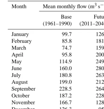
Qtend=0.3105x+143.38 (15) After defining the long period tendency (C1) for both series (base and future), the other components of the model were estimated based on the stationary series. The cyclic or sea-sonal component (C2m) was calculated as the mean of flows in each month (Table 1), in the base (1961–1990) and future periods (2011–2040).
[image:8.612.341.513.107.287.2]Then the time dependency component was modeled (C3), which represents the influence of the stream values of the
Table 1. Cyclic (seasonal) component in the base and future
peri-ods: mean monthly flow in the Ijuí River basin, Santo Ângelo sta-tion.
Month Mean monthly flow (m3s−1)
Base Future
(1961–1990) (2011–2040)
January 99.7 126.4
February 85.8 181.1
March 74.7 159.7
April 95.8 200.5
May 114.9 249.1
June 160.0 280.3
July 180.8 263.6
August 199.0 212.8
September 228.5 264.1
October 187.2 228.4
November 166.7 128.2
December 126.3 95.8
pmonths before the flow that occurs in the current time. At this stage, the correlation of flow in the current time (t) was analyzed in relation to the previous (t−1,t−2, . . . ,t−12), for each month, in the two stationary series (base and future) in which one can find, in general, a significant time depen-dency up to timet−3, characterizing a model of the third order.
In the multiplicative model, component C3 is a non-dimensional factor, with a mean equal to 1 along the hydro-logical series, obtained by the ratio between observed flow (stationary), in monthm, yeary, and mean flow in monthm
(C2m), as shown by Eq. (16). This equation can only be used when one has observed data. In the case of stochastic mod-eling, it is assumed that this non-dimensional factor depends only on the value of C3 in thepprevious months, thus al-lowing modeling component C3 at some time interval. The behavior of this component can be modeled by a multiple re-gression (Eq. 17) or even by a more complex structure, like an ANN with three input variables (Eq. 18).
C3=Qstm/y
C2m (16)
The random component (C4) is defined as the part that is not explained by the three other deterministic components, i.e., that represents the changes in hydrological behavior pro-voked by extreme events that occurred in the month. This part of the monthly flow is represented by the ratio between stationary flow (month,m, yeary) and the product of com-ponents C2 (monthm) and C3, as shown by Eq. (19). As in component C3, the values of C4 tend to a mean value close to 1.
C4= Qestm/y C2m·C3
(19) Next, aiming at the generation of synthetic series, first of all it was checked whether component C4 presented any pattern related to the deterministic portion of the model. Considering the stationary series of the base period (1961–1990), it was found that the value of C4 presented two slightly distinct pat-terns: (i) when the value of C3 is greater than 1, resulting in flow values higher than the monthly mean in the determinis-tic parcel of the model (high flow periods), the tendency of the random component C4 is to present less dispersed values, varying from 0.33 to 2.83, with a slightly lower mean (0.97); (ii) when the value of C3 is lower than 1, resulting in flows lower than the monthly mean in the deterministic portion of the model (low flow periods), the tendency of C4 is to present greater dispersion, varying from 0.21 to 7.24, with a slightly higher mean (1.03).
The most marked oscillations (inflections or impulses) in the monthly hydrogram, which depend on the random com-ponent C4, occur predominantly in dry periods, when the flow is below the mean observed for the month. This pat-tern observed in the historical series explains the smooth ten-dency found in the values of this component.
Also, considering the stationary series of the future pe-riod (2011–2040), when the value of C3 was higher than 1 (high flow periods), the random component C4 presented less dispersed values, ranging from 0.24 to 2.46, with a slightly lower mean (0.99). On the other hand, when the value of C3 was less than 1 (dry periods), component C4 oscillated be-tween 0.13 and 4.98, with a mean of 1.06.
Once the probability curves observed in both periods (base and future) had been observed, a few statistical distributions were adjusted (Gamma, log-normal, Weibull, among oth-ers) to the values of the random component C4. After the Kolmogorov–Smirnov adherence test was performed, it was found that the Gamma probability distribution with three parameters presented the best adjustment to the component modeled. The Gamma distribution with three parameters (ϑ,
η,β) is represented by the function given by Eq. (20).
fX(x)=
ζη−1e−ζ
ϑ 0(η) comζ= x−β
ϑ parax, ϑ eη >0, (20)
[image:9.612.310.546.71.232.2]whereϑ is a parameter of scale, with the dimensionx;β is a parameter of position, where β < x <∞, representing the
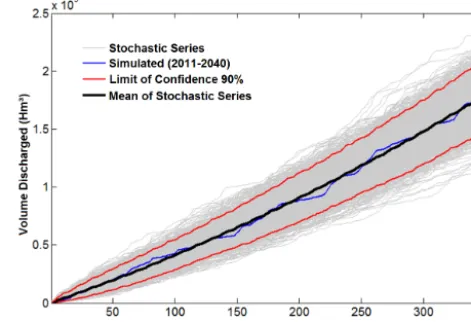
Figure 3. Curves of volume discharged in the future (2011–
2040) – difference between the original series (simulated) and the 1000 stochastic series generated – Ijuí River basin, Santo Ângelo gauge station.
smallest value ofx;ηis a shape parameter; and0(η)is the Gamma function, normally solved by numerical integration. After the adjustment of the four components, the stochas-tic series for both periods were generated, referenced to the parameters calculated based on the two monthly flow series (observed between 1961 and 1990, and simulated between 2011 and 2040). One-thousand series with an equal proba-bility of occurrence were generated for each period.
The stochastic modeling process was evaluated by com-paring the series generated and the series simulated in the future period, from the following aspects: (i) mean monthly flows; (ii) long period mean flow and volume discharged; (iii) standard deviation of monthly flows; and (iv) perma-nence curves.
The changes and uncertainties in water behavior were evaluated by comparing the stochastic series generated for the future period (2011–2040) and the series generated for the base period (1961–1990), considering central values and limits of confidence, looking at the following aspects: (i) mean monthly flows; (ii) standard deviation of monthly flows; (iii) long period mean flow and volume discharged; and (iv) permanence curves.
3 Results and discussions
This section will present the results and the discussions held concerning the analysis of stochastic modeling of monthly flows and the changes and uncertainties in water availability in the future period, between 2011 and 2040.
3.1 Stochastic modeling of monthly flows
be-Table 2. Difference between the original series (simulated) and the 1000 stochastic series generated – mean flow and monthly standard
deviation in the period between 2011 and 2040, Santo Ângelo gauge station.
Month Mean monthly flow (m3s−1) Monthly standard deviation (m3s−1)
Original Mean of Percentage Original Mean of Percentage
series series difference series series difference
generated generated
January 128.7 127.6 −0.83 % 118.0 102.5 −13.13 %
February 178.5 177.2 −0.74 % 179.3 142.2 −20.67 %
March 155.4 154.5 −0.62 % 143.7 124.0 −13.73 %
April 199.2 198.2 −0.48 % 163.2 158.8 −2.66 %
May 249.6 249.2 −0.16 % 168.0 211.2 25.70 %
June 276.5 276.5 0.01 % 195.0 224.0 14.87 %
July 262.5 262.9 0.16 % 183.5 213.4 16.29 %
August 217.7 218.3 0.27 % 149.4 175.5 17.44 %
September 268.1 269.5 0.52 % 205.2 216.6 5.54 %
October 228.9 230.6 0.72 % 183.9 188.0 2.24 %
November 126.9 128.0 0.86 % 83.8 104.2 24.43 %
December 97.0 97.9 0.93 % 87.8 78.9 −10.11 %
tween 2011 and 2040. Considering the mean of the 1000 se-ries generated for the future period, the long period mean flow (LPMF) was 200.3 m3s−1, only 1.1 m3s−1 (0.5 %) more than the simulated LPMF (original series). Figure 3 shows that this result was also reflected in the accumulated curve of the volume discharged. The mean difference be-tween the simulated curve (original series) and the central tendency of the 1000 curves generated (stochastic series) was only 4.8 %. Furthermore it can be seen that the smooth ten-dency of a long period was also preserved, and the values grew more markedly in the final half of the period.
Another characteristic maintained from the original series was the mean monthly flow. Table 2 shows that the mean absolute difference was only 0.52 %, considering the mean of the 1000 series generated for the period between 2011 and 2040. The greatest absolute difference between mean flows occurred in October, with an overestimation of 1.6 m3s−1.
Table 2 also shows that the monthly standard deviation was reasonably preserved, with a mean percentage absolute dif-ference of 13.9 % between the original series and the central tendency of the 1000 series generated. The smallest differ-ence was found in the month of October, and the greatest difference as to the monthly standard deviation was found in the month of May.
[image:10.612.125.472.95.291.2]Figure 4 illustrates the permanence curves of the mean monthly flow in the future period (2011–2040), in which the similarity between the original series and the central ten-dency observed in the stochastic series generated becomes clear. The greatest differences were observed in the ex-tremely high flows, with a permanence of less than 2 %. In the rest of the permanence intervals, the original curve was always located at the 90 % confidence interval defined by the red lines on the graph.
Figure 4. Permanence curves for the mean monthly flow between
2011 and 2040 – difference between the original series (simulated) and the 1000 stochastic series generated – Santo Ângelo gauge sta-tion.
3.2 Changes and uncertainties in water availability
In the Ijuí River basin, according to the climate scenario used, the annual accumulated rainfall will increase by 12.3 % between 2011 and 2040. This growth in volume of rainfall is mainly due to an increasing trend in rainfall between the months of January and June.
[image:10.612.312.545.319.466.2]Figure 5. Mean and 90 % confidence interval for the volume
dis-charged, based on the stochastic series generated, base period (1961–1990) and future period (2011–2040), Santo Ângelo gauge station.
confirmed by analyzing the changes related to the five cli-matic variables used to calculate evapotranspiration.
The first aspect analyzed as to changes and uncertain-ties regarding water availability in the future refers to the long period mean flow (LPMF) and to the volume dis-charged over the period of 30 years. On average, consider-ing the stochastic series in the base period (1961–1990), the LPMF was 41.6 m3s−1. The confidence interval of LPMF in the period, with a significance level of 0.1, was between 123.7 and 162.3 m3s−1 (range 38.6 m3s−1). On the other hand, in the future period (2011–2040), the projected LPMF was 200.3 m3s−1, considering the mean value found in the series. This value represents a mean increase of 41.4 % in the LPMF. The confidence interval of LPMF in the future, considering the same level of significance, will be between 165.1 and 233.6 m3s−1. Thus, the range of the interval will increase from 38.6 to 68.6 m3s−1.
The change of LPMF according to the projection for the future is also reflected by the mean of the total volume dis-charged over a 30-year period. Figure 5 shows that, between the years of 1961 and 1990, the mean of the total volume dis-charged was 132 566 Hm3. On the other hand, in the future period (2011–2040), the mean total volume discharged was 185 869 Hm3.
Considering the stochastic series in the future period, at a 0.1 level of significance, Fig. 5 shows that the total vol-ume discharged at the end of 30 years is at the interval be-tween 154 014 and 218 002 Hm3. This interval is broader and presents values much superior to those observed in the base period.
The second aspect analyzed refers to mean monthly flows. Figure 6 presents the mean and the 90 % confidence interval for the mean monthly flows, considering the 1000 stochastic series generated during the base and future periods.
The mean monthly flow will increase between the months of January and October, during the period between 2011 and 2040, compared to the base period, with percentages
Figure 6. Mean and 90 % confidence interval for the mean monthly
flows based on the stochastic series generated, during the base (1961–1990) and future periods (2011–2040), at Santo Ângelo gauge station.
that vary from 15 % (August) to 118 % (March). Besides the month of March, at least four other months will present a significant increase in mean flow: (i) February (113 %); (ii) May (110 %); (iii) April (101 %); and (iv) June (74 %). Considering a simple difference between the values obtained in the two periods, the months of May and June presented the greatest changes, with an increased mean monthly flow of 130 and 118 m3s−1, respectively. The reduction in mean monthly flow with percentages of 24 and 21 %, respectively, will only occur in the months of November and December.
Considering a statistical analysis of the 1000 stochastic se-ries generated for the two periods analyzed (base and future), at a 0.1 level of significance the confidence interval can be estimated that comprises the mean flow of each month. The greater the range of this interval, the greater also the uncer-tainty related to the mean monthly flow.
Figure 6 shows that the range of the 90 % confidence in-terval for the mean monthly flows will only be reduced in the months of November and December, thus following the tendency observed in the mean monthly values. In Novem-ber, for instance, the range of mean flow in the base period considering the series generated was 75 m3s−1. On the other hand, in the future period, the range of mean flows in this month was 64 m3s−1 (reduction of 16 % in the interval). In December, the range of the 90 % confidence interval for mean flow was reduced by 14 %, considering the two peri-ods.
[image:11.612.50.285.68.200.2]Table 3. Mean of standard deviation of monthly flows during the
base and future periods – Santo Ângelo gauge station.
Month Mean monthly standard deviation (m3s−1)
Base Future
(1961–1990) (2011–2040)
January 67.7 102.5
February 58.0 142.2
March 49.9 124.0
April 69.2 158.8
May 82.9 211.2
June 112.1 224.0
July 131.9 213.4
August 134.9 175.5
September 161.0 216.6
October 131.0 188.0
November 121.0 104.2
December 88.6 78.9
future period, the mean flow in May is inserted into the inter-val between 187 and 314 m3s−1(range of 127 m3s−1).
All the results of mean monthly flows presented indicate a significant change in the hydrological behavior of the Ijuí River basin, considering the climatic projection of the Eta model, between the months of February and June. Between the months of February and June, the confidence intervals do not present any overlap; i.e., the upper limit of the interval found in the base period is smaller than the lower limit of the interval found in the future.
The third aspect analyzed in the hydrological comparison between the base (1961–1990) and future (2011–2040) peri-ods was the standard deviation of mean monthly flows. As in the case of the averages of the flows in each month, con-sidering the central tendency of the 1000 series generated in the two periods, Table 3 illustrates that the standard deviation should increase between the months of January and October. The period of the year between the months of February and July is that one where the greatest change occurs in the dispersion of the flow values. Table 3 shows that in May, for instance, the standard deviation increases 155 % for the fu-ture. On the other hand, the month of November presents a smooth tendency to reduction in the flows, with a 121 m3s−1 reduction to 104 m3s−1(−14 %).
[image:12.612.85.251.96.289.2]When dividing the monthly standard deviation by the mean monthly flow, the coefficients of variation (CV) were obtained for both series, for each month. It can be seen that during the base period (1961–1990), the CV oscillated be-tween 0.7 (February) and 0.72 (November), while in the fu-ture period (2011–2040), the same index varied between 0.8 (April) and 0.85 (May). These results indicate a real increase in the monthly variability of flows, with greater fluctuations of monthly flows in the future.
Figure 7. Mean value of permanence curves of monthly flow
ac-cording to the stochastic series generated during the base (1961– 1990) and future periods (2011–2040), at Santo Ângelo gauge sta-tion.
Figure 8. 90 % confidence interval for the monthly flow
perma-nence curves, according to the stochastic series generated in the base (1961–1990) and future periods (2011–2040), at Santo Ângelo gauge station.
Another aspect analyzed as to changes in hydrological be-havior in the future refers to permanence curves of mean monthly flows. Figures 7 and 8, respectively, illustrate the mean value and confidence interval of 90 % for the perma-nence curves of monthly flow, considering the 1000 stochas-tic series generated in the base (1961–1990) and future peri-ods (2011–2040).
[image:12.612.312.541.289.445.2]The flow will be reduced in the future period only at per-manence intervals greater than 91 %, i.e., in the portion of lower flows that characterize dry periods. For flows with a permanence equal to or less than Q90 (intermediate and high flow), the tendency is toward increase in the flow val-ues (Fig. 7). As to the range of the 90 % confidence interval for the permanence curve of monthly flows (Fig. 8), the ten-dency is to increase in the future period, even the lower flow portion. This result illustrates an increase in the uncertainties associated with the estimate of the permanence curve in the future.
On average, considering all the series generated during the base and future periods, flow with a probability of ex-ceedance equal to or less than 99 % of the months (Q99) was 18 and 15 m3s−1, respectively. This indicates a mean reduction of 16 % inQ99 for the future period. Considering a statistical analysis of the stochastic series, at a 0.1 level of significance, we can say that Q99, during the period 1961– 1990, is located at the interval between 13.7 and 22.3 m3s−1 (range of 8.6 m3s−1). On the other hand, in the future period this interval changes to values between 10.4 and 20.4 m3s−1 (range of 9.9 m3s−1).
On average, considering all the series generated during the base (1961–1990) and future (2011–2040) periods, flow with a probability of exceedance equal to or less than 95 % of the months (Q95) was 30 and 28.5 m3s−1, respectively. This in-dicates a mean reduction of 5 % inQ95for the future period. This percentage is lower than that observed inQ99, illustrat-ing the tendency to inversion in the permanence curves for larger flows. As for the confidence interval of 90 % ofQ95, during the base period, the range was 10.4 m3s−1. On the other hand, in the future period, the range was 13.4 m3s−1.
In the base and future periods, the mean flow with a proba-bility of exceedance equal to or less than 90 % of the months (Q90) was 39.6 and 40.5 m3s−1, respectively. This shows a mean increase of 2 % inQ90 for the future period. As to the confidence interval of 90 % of Q90 in the base period, the range was 12.4 m3s−1. On the other hand, in the future pe-riod, the range was 18.4 m3s−1.
[image:13.612.311.545.66.433.2]In the base period (1961–1990), on average, the flow with a probability of exceedance equal to or less than 50 % of the months (Q50) was 108 m3s−1. At a 0.1 significance level, it can be said that Q50 in this period shows a range of 28 m3s−1. On the other hand, in the future period, on aver-age, the Q50 was much higher, with a values of 145 m3s−1, indicating a mean increase of 34 % for the future. As to the confidence interval, it can be said that the Q50, in the fu-ture period, will be between 116 and 178 m3s−1 (range of 62 m3s−1). Thus, the differences between the confidence in-tervals of Q50 in the two periods indicate a significant in-crease in the uncertainties associated with the permanence of flows in future. These results also illustrate a tendency to an increase in the differences between the flows of the base period and the future period inversely proportional to perma-nence.
Figure 9. Mean and 90 % confidence interval for the monthly flow
permanence curves at Santo Ângelo gauge station, according to the stochastic series generated in the base period (1961–1990) and fu-ture period (2011–2040): January, February, March and April.
In the portion of flows with permanence between 5 % (Q5) and 30 % (Q30), the confidence intervals (0.1 significance) of the two periods do not overlap; i.e., the upper limit of the in-terval during the base period is smaller than the lower limit of the interval in a future period. In the other portions of flows, even if significant differences have been found between the confidence intervals estimated in the base and future periods, they present an overlapping area.
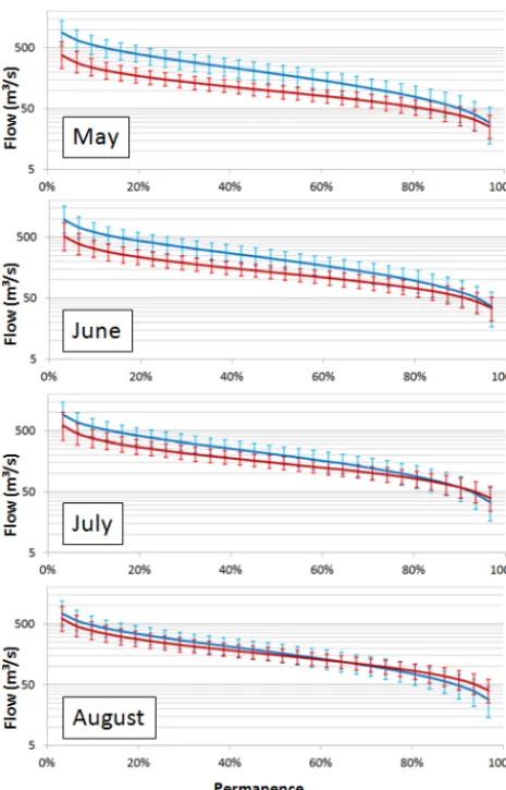
differ-Figure 10. Mean and 90 % confidence interval for the monthly flow
permanence curves at Santo Ângelo gauge station, according to the stochastic series generated in the base period (1961–1990) and fu-ture period (2011–2040): May, June, July and August.
ence of 130 m3s−1 between the permanence curves. Other months that call attention due to the great change in the per-manence curves for the future are June (118 m3s−1), April (99 m3s−1), February (94 m3s−1), March (84 m3s−1) and July (79 m3s−1).
Figures 9–11 illustrate the mean behavior and the 90 % confidence interval for the permanence curves of the monthly flows from January to December, for both periods (base and future). In general, it can be said, based on the results ob-tained, that between the months of January and October there is a tendency for the value of the flows with low permanence to increase – the high flow portion. Regarding this aspect, the main outstanding month is May, in which the mean flow with permanence equal to or less than 10 % (Q10) was 240 m3s−1 (base period) for 573 m3s−1 (future), which means an in-crease of 333 m3s−1(138 %) inQ10. Next, the other months between February and July are also outstanding, with an
in-Figure 11. Mean and 90 % confidence interval for the monthly flow
permanence curves at Santo Ângelo gauge station, according to the stochastic series generated in the base period (1961–1990) and fu-ture period (2011–2040): September, October, November and De-cember.
crease in the value ofQ10close to or higher than 200 m3s−1, as shown in Table 4.
Table 4 shows that between the months of February and June, the flows with a high permanence (portion of the lower flows) also presented higher values in the future period com-pared to the base period, indicating a tendency to a more gen-eralized increase in the flows for these months. In this case, in percentage terms, the month of March is outstanding, in which the mean flow with a probability of exceedance equal to or inferior to 90 % (Q90) was 22.8 m3s−1 (base period) to 34.5 m3s−1(future), representing an increase of 52 % in
Q90.
[image:14.612.311.546.64.427.2] [image:14.612.51.284.65.428.2]Table 4. Mean flows (m−3s−1) with 10 % (Q10) and 90 % (Q90) permanence during the base period (1961–1990) and future period (2011–2040), Santo Ângelo gauge station.
Month Base Future Changes Changes
(1961–1990) (2011–2040)
Q10 Q90 Q10 Q90 Q10 Q90
January 195.2 30.5 286.0 28.1 90.8 −2.4 February 168.6 26.8 393.5 39.2 224.9 12.4
March 145.3 22.8 343.0 34.5 197.7 11.7
April 201.4 31.7 438.1 44.4 236.7 12.7
May 240.4 38.7 573.0 50.2 332.6 11.5
June 324.0 51.5 610.5 61.6 286.5 10.1
July 376.5 58.9 582.9 58.2 206.4 −0.7
August 390.2 61.0 486.4 48.5 96.3 −12.5 September 463.6 72.6 594.5 60.9 130.9 −11.7 October 376.4 59.4 517.2 50.6 140.8 −8.8 November 345.7 54.1 284.6 28.1 −61.1 −26.0 December 252.2 39.8 217.1 21.6 −35.1 −18.2
[image:15.612.309.547.116.278.2]period (2011–2040) than those observed in the base period (1961–1990). In January, for instance, the results indicate a mean increase of 47 % inQ10 and an 8 % reduction inQ90 (Table 4).
In the months of November and December, the tendency observed is for a reduction in the flow values in general, both in the high flow portion and in the low flow portion. As shown in Table 4, in November the results indicate a mean re-duction of 18 % (−61 m3s−1) inQ10and 48 % (−26 m3s−1) inQ90. On the other hand, in December for the future period, the mean reduction inQ10andQ90was 14 % (−35 m3s−1) and 46 % (−18 m3s−1), respectively.
Tables 5 and 6 show the limits and ranges of the confi-dence interval of flows during the base and future periods, with a permanence of 10 % (Q10) and 90 % (Q90), respec-tively. In the case of the ranges of the confidence interval, each month, considering the 1000 stochastic series generated in both periods, there is a clear significant increase in the un-certainties related to the estimate of Q10 andQ90 between the months of January and October. The interval will only be reduced in the months of November and December.
In May, for instance, considering a level of significance of 0.1, the Q10 in the period between 2011 and 2040 is between 388.9 and 804 m3s−1, while during the period be-tween 1961 and 1990 the limits were 172.2 and 335.8 m3s−1. This considerable change in hydrological behavior can be ob-served also in the other months, especially between February and July, with growth rates greater than 100 % in the range of the 90 % confidence interval forQ10.
In general, the uncertainties regarding the hydrological be-havior in the future (2011–2040), taking a single climate sce-nario as reference, were greater than during the base period (1961–1990). This increase was reflected mainly between the months of January and October, as shown by the results of the
Table 5. Limits and ranges of the confidence interval of flows
(m3s−1) with a permanence of 10 % (Q10) during the base period (1961–1990) and future period (2011–2040), Santo Ângelo gauge station.
Month Base (1961–1990) Future (2011–2040)
Lower Upper Range Lower Upper Range
limit limit limit limit
January 136.3 275.3 139.0 196.3 395.4 199.0 February 117.6 232.6 115.0 272.3 548.0 275.7 March 102.5 201.3 98.9 236.7 474.6 238.0 April 141.3 285.0 143.8 305.4 620.1 314.7 May 172.2 335.8 163.6 388.9 804.0 415.1 June 229.6 451.4 221.8 420.1 855.8 435.7 July 261.9 526.2 264.3 403.8 790.2 386.4 August 274.1 541.5 267.4 333.8 679.1 345.3 September 325.1 648.0 323.0 400.7 828.7 428.0 October 269.3 515.8 246.5 352.6 723.1 370.5 November 245.4 485.3 239.9 197.1 400.5 203.3 December 174.3 352.6 178.3 151.6 297.3 145.7
Table 6. Limits and ranges of the confidence interval of flows
(m3s−1) with 90 % permanence (Q90) in the base period (1961– 1990) and future period (2011–2040), Santo Ângelo gauge station.
Month Base (1961–1990) Future (2011–2040)
Lower Upper Range Lower Upper Range
limit limit limit limit
January 20.4 42.9 22.5 16.6 43.3 26.7
February 17.9 38.0 20.1 23.8 60.0 36.2
March 15.2 32.0 16.8 20.5 53.6 33.0
April 21.5 43.7 22.2 26.1 68.9 42.8
May 25.9 53.3 27.4 29.8 80.1 50.3
June 34.6 71.3 36.7 35.7 95.3 59.6
July 38.9 83.4 44.4 34.4 87.7 53.3
August 41.4 85.3 43.9 28.7 72.9 44.2
September 48.9 100.1 51.2 37.0 93.9 56.9
October 39.6 82.5 42.8 30.9 77.4 46.6
November 35.8 76.3 40.4 16.6 43.6 27.1
December 26.5 55.9 29.4 12.9 32.5 19.6
comparative analysis between the permanence curves and the mean month flows and their confidence intervals.
The primary source of uncertainties is in the original hy-drological series itself, used in the stochastic modeling pro-cess. By formulating the stochastic model it is expected that the greater the mean monthly flow (seasonal component, C2), the greater also will be the possibility of obtaining extremely high flows. This occurs because the seasonal component is multiplied by the random component (C4) and the time de-pendence on (C3), which, although they have mean volumes close to 1, may possibly present extreme values.
[image:15.612.308.546.340.503.2]Figure 12. Relationship between the mean of the monthly flow and
the range of the confidence interval for the periods between 1961 and 1990 (base) and between 2011 and 2040 (future).
as the mean monthly flow increases. However, a clear dif-ference is also observed between the two straight lines that characterize the base and future periods. For the same mean monthly flow, the confidence interval range is higher in the future period series.
After a sensitivity analysis in the models based on ANN to determine the C3 component (time dependency) in both periods, it was found that in the future (2011–2040) the flow in time t is more sensitive because of the antecedent flows (t−1,t−2 andt−3). To illustrate this result, Fig. 13 shows the variation of the value of C3(t) because of the value of C3(t−1), and the variables C3(t−2) and C3(t−3) are maintained equal to 1, for both periods.
In the base period, between 1961 and 1990, even when an extremely low flow occurs in the previous month result-ing in a value close to 0 for variable C3(t−1), the calculated value of C3(t) is almost never less than 0.5, i.e., half the mean monthly flow. On the other hand, in the period between 2011 and 2040, due to the time sequence of the series and its char-acteristics, the value of C3(t) can be less than 0.3, giving rise to a value well below the mean of that month (Fig. 13).
The same pattern was observed for the portion of the ex-tremely high flows. During the period between 1961 and 1990, when there is a high flow in the previous months, re-sulting in a value of C3(t−1), for instance, 5 times higher than the monthly mean, the calculated value of C3(t) does not reach 2.2. In turn, during the future period, the value of C3(t) may be higher than 3.1, giving rise to a flow that is much higher than the monthly mean (Fig. 13).
In this way the component C3 presents greater fluctuations in the series between 2011 and 2040. This result helps ex-plain the greater variability found between the stochastic se-ries of the future period in relation to the base period.
Figures 14 and 15 illustrate the adjustment in the distribu-tion of Gamma probabilities for modeling the random com-ponent (C4) in situations of low flow (C3, in time t, less
[image:16.612.52.283.68.205.2]Figure 13. Variation of the value of C3(t), based on the value of C3(t−1), in modeling the time dependence component using ANN, keeping the other variables, C3(t−2) and C3(t−3), equal to 1 for the periods between 1961 and 1990 (base) and between 2011 and 2040 (future).
Figure 14. Adjustment of the Gamma distribution for the modeling
of the random component in a low flow situation, C3(t) less than 1, for the base and future periods.
than 1) and high flow (C3, in timet, higher than 1), respec-tively.
In general, it is possible to observe that the behavior found in the base series (1961–1990) of the random component C4 was maintained in the series of the future period (2011– 2040), especially as regards the months in which the value of C3 was less than 1 (Fig. 14), resulting in a flow lower than the monthly mean. In this case, considering the base and future periods, the chance of the value drawn for C4 being greater than 1 was 42 and 43.5 %, respectively.
On the other hand, in the months when the time depen-dence component (C3) surpassed the value of 1, the differ-ence between the series was slightly higher (Fig. 15). The probability of a value higher than 1 being drawn for com-ponent C4 was 38 and 43 %, respectively, for the base and future series.
[image:16.612.310.546.286.411.2]Figure 15. Adjustment of the Gamma distribution for the
model-ing of the random component in a high flow situation, C3(t) higher than 1, for the base and future periods.
besides the mean and the dispersion of the data being greater than in the base period, provoking more abrupt fluctuations in the flow values, the correlation coefficient between the flows at timest andt−1 was quite high (mean 0.66), with values between 0.5 (November) and 0.78 (March). Already in the period between 1961 and 1990, the correlation coefficient values were between 0.26 (June) and 0.75 (February), with a mean equal to 0.54.
Considering the methodology adopted to model flows in future and to generate the stochastic series, it can therefore be said that there is a certain tendency to an increased hydro-logical variability during the period between 2011 and 2040, with a greater dispersion of values in relation to the monthly mean. This finding implies greater uncertainty regarding the availability of water in the future, with the possible occur-rence of time series that are very different from each other.
4 Conclusions
This study analyzed the possible changes and uncertainties related to water availability in the future using a stochastic approach, based on the climate change scenario originating in the LOW member of the Eta CPTEC/HadCM3 climate model, for the period between 2011 and 2040. The study was applied to the Ijuí River basin, in the south of Brazil. The methodology involved the correction of the climate vari-ables projected for the future, the hydrological simulation to define a series of monthly flows, and stochastic modeling to generate 1000 hydrological series with an equal probability of occurrence.
As to the stochastic model to generate monthly flow series, several characteristics of the original series were preserved, simulated for the period between 2011 and 2040. Outstand-ing among them are LPMF and the mean monthly flows, both with differences of only 0.5 %. The monthly standard devi-ation was reasonably preserved, with a mean percentage ab-solute difference of 13.9 % between the original series and the central tendency of the 1000 series generated. The
simi-larities between the permanence curves of the monthly flows of the original series and the central tendency observed in the stochastic series generated also became clear. Based on all these results it can be concluded that the stochastic model proposed is adequate to generate monthly flow series.
Various results showed a tendency to increased flows in a general context. The LPMF, for instance, presented an alteration from 141.6 m3s−1 (1961–1990) to 200.3 m3s−1 (2011–2040), which is a mean increase of 41.4 % in LPMF. Comparing the two periods, the difference between the to-tal volume discharged in 30 years was 53 303 Hm3. It could also be seen that the mean flow and the monthly standard deviation increased between the months of January and Oc-tober in the period between 2011 and 2040. Between the months of February and June, the percentage increase in the mean monthly flow was greater than 100%. It was also found that, in the base period (1961–1990), the coefficient of vari-ation (CV) oscillated between 0.698 (February) and 0.716 (November), while for the future period (2011–2040), the same index varied from 0.801 (April) to 0.848 (May), in-dicating a real increment in the monthly variability of flows, with greater fluctuations in future flows.
Based on the comparison of the permanence curves of monthly flow between the base and future periods, it is con-cluded that the flow presented lower values (−5.1 %) only at permanence intervals greater than 90 % in the dry months. For flows with a permanence equal to or less thanQ90 (inter-mediate and high flow), there is a tendency for the flow val-ues to increase. For instance, in the base period (1961–1990), on average, the flow with permanence equal to or less than 50 % of the months (Q50) was 108.2 m3s−1. On the other hand, in the future periodQ50was much higher, with a value of 145.1 m3s−1(34.2 % increase).
It can also be observed that the smaller changes in flow permanence occurred between the months of August and Jan-uary. On the other hand, in the other months, the changes were drastic. In May, for instance, an absolute mean dif-ference was found of 130.5 m3s−1between the permanence curves.
In general it is concluded, based on the results obtained, that between the months of January and October there is a tendency for the flood flows to increase. Between the months of February and June, the flows with high permanence (min-imum flows) also presented higher values in the future com-pared to the base period. On the other hand, in the months of January, July, August, September and October, even lower minimum flow values were observed, indicating that in these months there is a tendency to amplify the extreme values. Finally, in the months of November and December, the ten-dency observed is for the reduction of flow values, in general, both in the high flow and in the low flow portions.