www.hydrol-earth-syst-sci.net/21/1063/2017/ doi:10.5194/hess-21-1063-2017
© Author(s) 2017. CC Attribution 3.0 License.
On the consistency of scale among experiments,
theory, and simulation
James E. McClure1, Amanda L. Dye2, Cass T. Miller2, and William G. Gray3
1Advanced Research Computing, Virginia Tech, Blacksburg, Virginia 24601-0123, USA
2Department of Environmental Sciences and Engineering, University of North Carolina, Chapel Hill,
North Carolina 27599-7431, USA
3Curriculum for the Environment and Ecology, University of North Carolina, Chapel Hill, North Carolina 27599-3135, USA
Correspondence to:William G. Gray ([email protected])
Received: 31 August 2016 – Discussion started: 15 September 2016
Revised: 17 January 2017 – Accepted: 20 January 2017 – Published: 20 February 2017
Abstract.As a tool for addressing problems of scale, we con-sider an evolving approach known as the thermodynamically constrained averaging theory (TCAT), which has broad ap-plicability to hydrology. We consider the case of modeling of two-fluid-phase flow in porous media, and we focus on issues of scale as they relate to various measures of pres-sure, capillary prespres-sure, and state equations needed to pro-duce solvable models. We apply TCAT to perform physics-based data assimilation to understand how the internal be-havior influences the macroscale state of two-fluid porous medium systems. A microfluidic experimental method and a lattice Boltzmann simulation method are used to examine a key deficiency associated with standard approaches. In a hy-drologic process such as evaporation, the water content will ultimately be reduced below the irreducible wetting-phase saturation determined from experiments. This is problematic since the derived closure relationships cannot predict the as-sociated capillary pressures for these states. We demonstrate that the irreducible wetting-phase saturation is an artifact of the experimental design, caused by the fact that the bound-ary pressure difference does not approximate the true capil-lary pressure. Using averaging methods, we compute the true capillary pressure for fluid configurations at and below the irreducible wetting-phase saturation. Results of our analysis include a state function for the capillary pressure expressed as a function of fluid saturation and interfacial area.
1 Introduction
Complementing the advancing ability of experimental study is the development of simulation tools for various as-pects of hydrologic systems that make use of advanced com-puter technology (e.g., Miller et al., 1998, 2013; Flint et al., 2013; Kauffeldt et al., 2016; Paiva et al., 2011; Dietrich et al., 2013; Zhou and Li, 2011; Bauer et al., 2015; Dudhia, 2014). These models of watersheds, rivers and estuaries, and subsur-face regions usually make use of traditional equations with the advances occurring through the ability of modern com-puter architecture to handle larger problems using parallel computing and more elegant, efficient graphical user inter-faces.
A third element of advancing modeling of water resources systems is the development of theory that accounts for phys-ical processes. On one hand, forming theoretphys-ical advances for mechanistic models based upon conservation equations can be viewed as the standard challenges of accounting more completely for conserved quantities and of developing clo-sure relations for dissipative processes. However, the need to pose closure relations at scales that are consistent with those at which the problems have been formulated creates a need for a variety of constitutive proposals. Furthermore, consistency of models requires that equation formulations be consistent across scales such that variables developed at a smaller scale can inform the equations employed at a larger scale. Overall, these considerations lead to identifying scale and scaling behavior in both time and space as important challenges in posing models (Wood, 1995; Wang et al., 2006; Skøien et al., 2003; Pechlivanidis et al., 2011; Gleeson and Paszkowski, 2014; Gentine et al., 2012; Blöschl, 2001).
In an era of unprecedented data generation, opportunities to use multiscale averaging theory to develop physics-based data assimilation strategies have never been more evident. The challenge of performing meaningful theoretical, exper-imental, and computational analyses is constrained by the need to ensure that the length and timescales of quantities arising in each approach can be related. The scales of experi-mental data, variables appearing in equations, and computed quantities must be the same if they are to be compared in any meaningful way. As a prerequisite for this to happen, data generated by any of the methods must be consistent across the range of scales considered (Ly et al., 2013; Kauffeldt et al., 2013).
While the desire for consistencies across scales and ap-proaches is conceptually simple to understand, it has proven to be a difficult practical objective to meet. The change in scale of conservation and balance equations can be accom-plished rather easily. The problem with applying these equa-tions lies in the aforementioned need to average some in-tensive variables, the requirement that closure conditions be proposed at the larger scale, and the need to account for the dynamics of new quantities that arise in the change of scale. Without accounting for all of these items properly, models are doomed to fail. An essential element in ensuring success is the averaging of thermodynamic relations to the
larger scale (Gray and Miller, 2013). This provides linkage of variables across scales and also ensures that all physical processes are properly accounted for. For modeling rainfall– runoff processes, Wood et al. (1988) proposed the use of a representative elementary area as a portion of a watershed over which averaging can occur to develop a model. This idea was extended and applied by Blöschl et al. (1995). Sub-sequently, Reggiani et al. (1998) proposed treating a hydro-logic system as a collection of interconnected lumped ele-ments. The lumping was accomplished by integration over individual portions of the system with distinct properties, e.g., aquifers, streams, channels. This effort did not include integration of thermodynamic relations, and as a result did not properly account for the impact of gravitational potential in driving flow between system elements. An effort to ad-dress this shortcoming by a somewhat ad hoc introduction of gravitational forces (Reggiani et al., 1999) was only partially successful. Averaging of thermodynamic relations to lumped elements has since been presented (Gray and Miller, 2009).
Challenges in assuring consistency across scales have also been confronted in the modeling of porous medium sys-tems. Special challenges have been encountered for two-fluid-phase flow, where upscaling leads to the introduction of quantities such as specific interfacial area, which is the area where two phases meet normalized by the volume of the region, and specific common curve length, which is length of a curve where three phases meet normalized by the volume of the region. Modeling of multiscale porous medium sys-tems must also employ thermodynamics that is scale consis-tent and included naturally as a part of the process. Because of the inability to overcome these challenges, most efforts to model multiscale, multiphase porous medium systems do not have thermodynamic constraints and full-scale consistency that would be expected in mature models. The thermody-namically constrained averaging theory (TCAT) approach is relatively refined and provides means to model systems that are inherently multiscale in nature and also to link disparate length scales, while representing the essential physics natu-rally and hierarchically with varying levels of sophistication. However, realizing these scale-consistent attributes requires new approaches, new equations of state, novel parameteriza-tions, and, as with any new model, evaluation and validation.
2 Objectives
ex-ploited to understand and characterize how phase connectiv-ity influences key macroscale quantities. In other words, we ensure consistency between information at small and large scales by using precise mathematics to change the scale of variables; and we also ensure that variables denoted as per-taining to theory, experiment, or simulation are defined such that they refer to quantities defined at the same scale and are directly comparable. The specific objectives of this work are – to formulate explicitly related microscale and macroscale descriptions of state variables impor-tant for traditional and evolving descriptions of capillary pressure
– to determine state variables for capillary pressure us-ing complementary experimental and computational ap-proaches
– to compare a traditional state equation approximation approach with a carefully formulated approach based in multiscale TCAT theory
– to demonstrate the limitations of traditional state equa-tion approaches for macroscale capillary pressure and – to examine the uniqueness of alternative state equation
formulations for capillary pressure.
The objectives of this work are focused on a specific as-pect of approaches commonly used to represent the behav-ior of porous medium systems. The physical size of the systems considered experimentally and computationally are small and idealized compared to field-scale hydrologic sys-tems that motivate this work and which hydrologists collec-tively endeavor to better understand and describe quantita-tively with higher fidelity than current approaches. Our hope in examining these fundamental issues is to advance basic understanding of hydrologic systems and to stimulate future work that might allow such advancements to be reduced to improved tools for practice in due course.
3 Background
Two spatial scales are of primary interest for the porous medium problems of focus herein: the microscale, which is often referred to as the pore scale; and the macroscale, which is often referred to as the porous medium continuum scale. At the microscale, the geometry of all phase distributions are fully resolved in space and in time, which makes it possi-ble to locate interfaces where two phases meet and common curves where three phases meet. The equations governing the conservation of mass, momentum, and energy, the bal-ance of entropy, and equilibrium thermodynamic relations are well established at the microscale. Microscale experi-mental work and modeling are active areas of research be-cause of their relevance to understanding operative processes
in complex porous medium systems that were previously im-possible to observe. The macroscale is a scale for which a point is associated with some averaged properties of an av-eraging region comprising all phases, interfaces, and com-mon curves present in the system. Notions such as volume fraction and specific interfacial area arise when a system is represented at the macroscale in terms of averaged measures of the state of the system. These additional measures are quantities that must be determined in the model solution pro-cess. Because of historical limitations on both computational and observational data, the macroscale has been the tradi-tional scale at which models of natural porous media systems have been formulated and solved. Closure relations at this scale are needed to yield well-posed models. Traditionally, these closure relations have been posited empirically and pa-rameter estimation has been accomplished based upon rela-tively simple laboratory experiments. In general, traditional macroscale models, while the dominant class of model, suf-fer from several limitations related to the way in which such models are formulated and closed (Gray and Miller, 2014). A precise coupling between these disparate length scales has usually been ignored.
As efforts to model and link hydrologic elements in mod-els advance, the ability to address scales effectively will become essential. For porous media, methods such as av-eraging, mixture theory, percolation theory, and homoge-nization have been employed to transform governing sys-tem equations from smaller to larger length scales (Hornung, 1997; Panfilov, 2000; Cushman, 1997). The goal of such ap-proaches is to transform small-scale data to a larger scale such that it can be used to inform models that have been ob-tained by consistent transformation of conservation and bal-ance equations across scales.
Averaging procedures have been used for analysis of porous media for approximately 50 years (e.g., Bear, 1972; Anderson and Jackson, 1967; Whitaker, 1986, 1999; Marle, 1967). The methods of averaging can be applied to single-fluid-phase systems as well as to multiphase systems. Suc-cess in the development of averaging equations for single-fluid-phase porous media to obtain equations such as Darcy’s law has been achieved (e.g., Bachmat and Bear, 1964; Whitaker, 1967; Gray and O’Neill, 1976). These instances did not so much derive a flow equation as show that a com-monly used flow equation could be obtained using averag-ing theorems and appropriate assumptions. Thus, these early efforts did not contribute significantly to objective develop-ment of flow equations that seek to capture important physi-cal processes. They do serve to provide a systematic frame-work for developing larger-scale equations. Work for two or more fluid phases in porous media has proven to be more difficult and has not been as illuminating.
to account for system kinematics, and (4) challenges repre-senting other important physical phenomena explicitly, such as contact angles and common curve behavior. These four difficulties sometimes impact the system description in com-bination.
Multiple-fluid-phase porous media differ from a single-fluid-phase porous medium system by the presence of the interface between the fluids. This interface is different from a fluid–solid interface because of its dynamics. The total amount of solid surface is roughly constant, or is slowly vary-ing, for most natural solid materials. The fluid–fluid-specific interfacial area changes in response to flow in the system and redistribution of phases. The timescale of this change is between that of the pore diameter divided by flow veloc-ity and that of pore diameter divided by solid phase move-ment. These specific interfacial areas are important for their extent, surface tension, and curvature. They are the location where capillary forces are present. Thus, a physically con-sistent model must account for mass, momentum, and en-ergy conservation at the interfaces; a model concerned only with phase behavior cannot represent capillary pressure in a mechanistically high-fidelity fashion (Gray et al., 2015). This shortcoming is evidenced, in part, by multi-valuedness when capillary pressure is proposed to be a function only of satu-ration (Albers, 2014).
Intensive variables that are introduced at the macroscale without consideration of microscale precursor values are also poorly defined. For example, a range of procedures for aver-aging microscale temperature can be employed that will lead to different macroscale values unless the microscale tem-perature is constant over the averaging region. Thus, mere speculation that a macroscale value exists fails to identify how or if this value is related to unique microscale variables and most certainly does not relate the macroscale variable to microscale quantities. The absence of a theoretical rela-tion makes it impossible to reliably relate microscale mea-surements to larger-scale representations (Essex et al., 2007; Maugin, 1999). Further confusion arises when pressure is proposed directly at the macroscale. Microscale capillary pressure is related to the curvature of the interface between fluid phases and does not depend on the pressures in the two phases themselves. At equilibrium, microscale capillary pressure becomes equal to the difference between phase pres-sures at the interface. Proposed representations of macroscale capillary pressure often specify that the capillary pressure is equal to the difference in some directly presumed quantities known as macroscale pressures of phases. These representa-tions ignore both interface curvature and the fact that only when evaluated at the interface is the phase pressure use-ful for describing equilibrium capillary pressure. This is es-pecially problematic when boundary pressures in an experi-mental cell are used to compute a “capillary pressure”. Note that under these common experimental conditions, regions of entrapped wetting phase are not in contact with the non-wetting fluid that is observed on the boundary of the system.
The importance of kinematics is recognized, at least im-plicitly, in modeling many systems at reduced dimensionality or when averaging over a region the system occupies. For ex-ample, in the derivation of vertically integrated shallow wa-ter flow equations, a kinematic condition on the top surface is imposed based on the condition that no fluid crosses that sur-face (Vreugdenhil, 1995). Macroscale kinematic equations for interfaces between fluids in the absence of porous me-dia have been proposed in the context of boiling (Koca-mustafaogullari and Ishii, 1995; Ishii et al., 2005). Despite the fact that interface reconfiguration has an important role in determining the properties and behavior of a multi-fluid porous medium system, attention to this feature is extremely limited (Gray and Miller, 2013; Gray et al., 2015). In some cases, models of two-fluid-phase flow in porous media have been proposed that do not account for either system kine-matics or for interfacial stress (e.g., Niessner et al., 2011). Both are necessary components of physically realistic, high-fidelity models.
The mixed success in posing appropriate theoretical mod-els, making use of relevant data, and harnessing effective computer power to advance understanding of hydrologic sys-tems is attributable to the inherent difficulty of each of these scientific activities. For progress to be made in enhancing un-derstanding, a significant hurdle must be overcome that re-quires consistency among these three approaches and within each approach individually. We have found that by perform-ing complementary microscale experimental and computa-tional studies, we have formed a basis for being able to up-scale data spatially with insights into the operative timeup-scales for the system (Gray et al., 2015). The small-scale data sup-port our quest for larger-scale closure relations and elimi-nates confusion about concepts such as capillary pressure as a state function and dynamic processes that cause changes in the value of capillary pressure. Key to being able to develop faithful models are consistent scale change of thermody-namic relations and implementation of appropriate kinematic relations. The approach of combining sound theory, modern experimental techniques, and advanced computational tech-niques to the study of environmental systems has applicabil-ity not only for the porous media systems emphasized here but also for large-scale systems with interacting atmospheric, surface, and subsurface elements.
4 Theory
using microtensiometers cannot resolve the issues of concern identified in this work. The differences among approaches are important, and commonly used approaches are flawed. In the formulation that follows, we show how microscale pres-sures can be averaged in a variety of ways as well as the relationship of these averaged pressures to the true capillary pressure. We note that averaging of pressures is inherent in the formulation of macroscale models; and indeed measure-ment devices themselves provide averages over a length scale depending upon the device. The issues related to averaging cannot be avoided.
Averaging of any intensive variable (e.g., pressure, tem-perature, chemical potential) is problematic because there is no unique averaging procedure that can be employed. This is in contrast to obtaining an upscaled value of mass per volume by integrating the microscale density over a volume to ob-tain the total mass and then dividing by the volume to get the upscaled density. Pressure, for example, is a force per area or, alternatively, an energy per volume. Averaging pressure over some area in a region as opposed to averaging over the volume of the region can give different values. Thus, it is im-perative to identify pressure averages in ways that they arise in equations and in data collection. Correct identification of an averaged pressure and association of that average with a particular process or element of an equation is essential if the physics of a system are going to be described well at the macroscale. For this reason, we carefully define the larger-scale variables that will be used in analyzing the simulated system and describing system physics in this section. We also highlight the importance of identifying capillary pressure as an intrinsic property of an interface rather than as having an identity that is based on properties of juxtaposed phases.
Direct upscaling can be performed based on microscale information, providing an opportunity to explore aspects of macroscale system behavior that have previously been overlooked. Underpinning this exploration is the precise definition of macroscale quantities. TCAT models are de-rived from first principles starting from the microscale. At the macroscale, important quantities such as phase pres-sures, specific interfacial areas, curvatures, and other aver-aged quantities are defined unambiguously based on the mi-croscale state (e.g., Gray and Miller, 2014). For the two-fluid-phase flow, we consider the wetting phase (w), the non-wetting phase (n), and the solid phase (s) within a domain. Each phase occupies part of the domain,α, whereα= {w,
n,s}. The intersection between any two phases is an inter-face. The three interfaces are denoted bywnws, andns.
Finally, the common curve wns is defined by the juncture
of all three phases. The TCAT two-phase model is developed based on averaging with the complete set of entities, with the index setJ= {w,n,s,wn,ws,ns,wns} =JP∪JI∪JC
cho-sen to include all three phasesJP= {w,n,s}, the interfaces JI= {wn,ws,ns}, and the common curveJC= {wns}. Based
on this, the pore space is defined as the union of the domains for the two fluidsDf=w∪n.
Macroscale quantities can be determined explicitly from microscale information based on averages. In this work, the form for averages is
hPiα,β=
R
α Pdr
R
β
dr , (1)
whereP is the microscale quantity being averaged. The do-mains for integration can be the full domain, the entity domainsα for α∈J, or their boundary 0α. The bound-ary of an entity can be further sub-divided into an internal component 0αi and an external component 0αe, which
to-gether yields0α=0αi∪0αe. The external boundary is
sim-ply0αe=α∩0.
The volume fractions, specific interfacial areas, and spe-cific common curve length are each extent measures that can be formulated as
α= h1iα,. (2)
The volume fractions correspond toα∈JP; specific
interfa-cial areas correspond to averaging over a two-dimensional interface forα∈JI; and the specific common curve length
corresponds to averaging over a one-dimensional common curve forα=wns. The system porosity,, is directly related to the solid-phase volume fraction by
=1−s. (3)
The wetting-phase saturation,sw, can also be expressed in terms of the extent measures,
sw=
w
1−s =
w
. (4)
At the macroscale, various averages arise for the fluid pres-sures. For flow processes, the relevant quantity is an intrinsic average of the microscale fluid pressure,pα, expressed as
pα= hpαiα,α (5)
for α∈Jf, which is the index set of fluid phases. In most
laboratory experiments phase pressures are measured at the boundary. Pressure transducers can be placed within a do-main at pre-selected locations, which still does not provide a dense, non-intrusive measure of fluid pressure at all lo-cations, including along interfaces. The associated average pressure for the intersection of the boundary of the phase with the exterior of the domain is
p0α = hpαi0αe,0αe (6)
forα∈Jf.
The curvature of the boundary of phase β is defined at the microscale as
Jβ= ∇0·nβ, (7)
where∇0=(I−nβnβ)· ∇ is the microscale divergence op-erator restricted to a surface,Iis the identity tensor, andnβis the outward normal vector from theβ phase. Since the inter-nal boundary is an interface, the curvature of a phase bound-ary is also the curvature of the interface between phases for locations within the domain. At the microscale, the capillary pressure is defined at the interface between fluid phases as
pwn= −γwnJw, (8)
where γwn is the interfacial tension of the wn interface.
Laplace’s law is a microscale balance of forces acting on an interface that relates the capillary pressure to the difference between the microscale-phase pressures evaluated at the in-terface with
pn−pw= −γwnJw. (9)
It is important to understand that Laplace’s law applies at points on thewninterface only at equilibrium; the definition of capillary pressure given by Eq. (8) applies even when the system is not at equilibrium. Additionally, if the mass per area of the interface is non-zero, Laplace’s law must be mod-ified to account for gravitational effects (Gray and Miller, 2014). Care must be taken when extending this relationship to the macroscale, as is shown below.
Since the capillary pressure is defined for the interface be-tween the two fluids, wn, we consider an average of the
microscale curvature based on this entity
Jwwn= hJwiwn,wn= −hJniwn,wn. (10)
Similarly, the macroscale capillary pressure is
pwn= −hγwnJwiwn,wn. (11)
The case of a constant interfacial tension at the microscale allows for
pwn= −γwnJwwn. (12)
In the context of Eq. (9), a third pressure of interest for the two-fluid-phase systems is the interface-averaged pressure
pwnα = hpαiwn,wn (13)
for α∈Jf. A macroscale version of Laplace’s law can then
be written as
pwnn −pwnw = −γwnJwwn. (14) At equilibrium, Laplace’s microscale law will hold every-where on wn. This implies that Eq. (14) must also be
sat-isfied at equilibrium for the case of a constant interfacial
tension. However, measurements of pwnw andpnwn must be performed at the interface wn. This is not practical, and
perhaps not even useful since neither quantity appears in macroscale models. At the macroscale, it is most convenient to work in terms of averaged phase pressurespw andpn. Becausepα andpwnα are not equivalent, the way in which Eq. (14) can be used is in question. In this work, we explore this dilemma, giving special consideration to the connectivity of the wetting phase.
In previously published work, we have considered the im-pact of non-wetting-phase connectivity in detail (McClure et al., 2016b). The connectivity-based analysis presented in that work can be used to re-cast Eq. (14) in terms of the connected wetting-phase regions. These regions are identi-fied by sub-dividingwintoNw sub-regions that do not
in-tersect. The sub-regions cannot touch each other, meaning thatwi∩wj=Ø for alli6=j withi,j∈ {1, 2, . . . Nw}
where the overbar on denotes a closed domain that in-cludes explicitly the boundary. Interfacial sub-regions are formed from the intersectionwin=wn∩wi. When the
non-wetting phase is fully connected, an approximate ver-sion of Laplace’s law can be derived as
pn−pwi= −γwnJwin
w , (15)
fori∈ {1, 2, . . . ,Nw}. This expression relates the
average-phase pressures within each region of wetting average-phase to the curvature of the adjoining interface. The average-phase pres-sures are defined as
pwi= hp
wiwi,wi, (16)
and the average curvature as
Jwin
w = hJwiwin,wi n. (17)
The quantitiespwiandJwin
w are averaged quantities, but they
are not macroscale quantities. The macroscale pressure of the wetting phase can be determined as
pw= 1
w
Nw
X
i=1
wipwi, (18)
and the macroscale capillary pressure is
pwn= −γ
wn
wn
Nw
X
i=1
winJwin
w . (19)
For the case where multiple disconnected sub-regions are present for either phase, the relationship betweenpn−pw
The definitions of pressures provided demonstrate that several different pressures are of interest for two-fluid sys-tems. In general these pressures will not be equivalent. Thus, care is needed in analyzing the system state and in proposing relations among pressures. Typically only the pressure de-fined by Eq. (6) is measured in traditional laboratory exper-iments, and this is often true even with state-of-the-science experiments that include high-resolution imaging. On the other hand, computational approaches provide a means to compute all of the defined pressures, yielding a basis to de-duce a more complete understanding of the macroscale be-havior of the system than would be accessible using ap-proaches that are only able to control and observe fluid pres-sures on the boundaries of the domain. Further, the formula-tion detailed above applies for dynamic condiformula-tions as well as equilibrium or steady-state conditions except where specifi-cally noted. For dynamic conditions, the averaged quantities are computed at some instant in time.
5 Materials and methods 5.1 Experimental design
An experimental approach was sought to investigate the dis-tribution of capillary pressure in a porous medium system. To meet the objectives of this work, we needed directly to observe capillary pressure at high resolution, which requires computation of the average curvature of the fluid–fluid in-terface as a function of the averaging region. Because we wished to observe systems at true equilibrium and knew from recent experience that extended periods of time are neces-sary to obtain such a state (Gray et al., 2015), we elected to rely upon a microfluidic approach for which we could verify true equilibrium states were achieved. Microfluidic devices are physically small but can be made sufficiently large to sat-isfy the conditions for being a valid macroscale representa-tive elementary volume (REV). This is so because the sys-tems are well above the microscale continuum limit and then only need to satisfy the conditions for the size being a rep-resentative sampling of the pore morphology and topology of the media. The size needed for an REV has been investi-gated previously for two-fluid-phase flow. Typically in three-dimensions, a few thousand spheres is needed to produce es-sentially invariant information for quantities such as satura-tions, interfacial areas, and capillary pressure. This translates to slightly over 10 mean grain diameters in each dimension. Microfluidic cells can be fashioned to meet this requirement. Even though hydrologic problems motivate this work, the fundamental nature of the capillary pressure state function can be investigated with any pair of immiscible fluids. Mini-mizing the mutual solubilities of each fluid in the companion fluid is an important design characteristic that can simplify the experimental work without loss of generality. Thus, phys-ically small microfluidic systems that did not include water
Non-wetting-fluid-phase reservoir
Wetting-fluid-phase reservoir
Porous medium cecll
500 µm
[image:7.612.309.542.65.173.2]525 µm
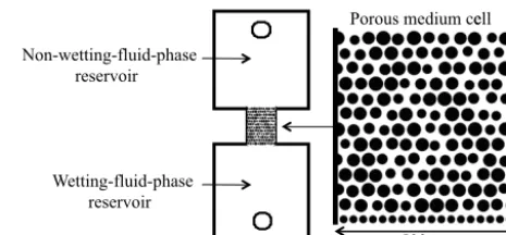
Figure 1.A depiction of the two-dimensional micromodel that was
used in the displacement experiment. The solid phase consists of pore-space-free solid cylinders of varying radii distributed in the horizontal plane represented by black and the regions accessible to fluid flow by white within the porous medium cell.
were used in this work, which might on the surface appear to be far removed from the motivating hydrologic systems of concern.
in-cremental change in pressure step was applied. The drainage process was terminated prior to nitrogen breakthrough into the decane reservoir.
The solid geometry used in our microfluidic experiments was designed to allow for high capillary pressure at the end of primary drainage. At the wetting-fluid-phase reservoir, a layer of evenly spaced homogeneous cylinders was placed such that the gap between cylinders was uniformly small. This allowed for a large pressure difference between the fluid reservoirs, since the non-wetting fluid phase did not penetrate the wetting-fluid-phase reservoir over a wide range of pres-sure differences.
5.2 Computational approach
The experimental microfluidics setup described in the previ-ous section provides a way to perform traditional two-fluid-flow experiments and observe the internal dynamics of in-terface kinematics and equilibrium distributions. Microscale-phase configurations can be observed directly, and averaged geometric measures can be obtained from this data. While boundary pressure values are known, the experiment does not provide a way to measure the microscale pressure field. Accurate computer simulation of the experiment can pro-vide this information and can also be used to generate addi-tional fluid configurations that may not be accessible exper-imentally. In particular, configurations below the irreducible wetting-phase saturation will be considered. The common identification of a saturation as “irreducible” is a misnomer because wetting-phase saturations beneath this value can be achieved through, for example, evaporation or by initializ-ing a saturation below this value in an experimental setup. In this work, simulation is applied in two contexts: (1) to sim-ulate the microscale pressure field based on experimentally observed fluid configurations, and (2) to simulate two-fluid equilibrium configurations based on random initial condi-tions. Success with the first set of simulations in matching the experiments provides confidence that the results of the second set of computations represent physically reasonable configurations. Here we summarize each of the approaches.
Simulations are performed using a “color” lattice Boltz-mann method (LBM). Our implementation has been de-scribed in detail in the literature (see McClure et al., 2014a, b). The approach relies on a multi-relaxation time scheme to model the momentum transport. In the limit of low Mach number, the implementation recovers the Navier–Stokes equations with additional contributions to the stress tensor in the vicinity of the interfaces. The interfacial stresses between fluids result from capillary forces, which play a dominant role in many two-fluid porous medium systems. The formu-lation relies on separate lattice Boltzmann equations (LBEs) to recover the mass transport for each fluid. This decouples the density from the pressure to allow for the simulation of incompressible fluids. Our implementation has been ap-plied to simulate two-fluid-phase flows in a variety of porous
medium geometries, recovering the correct scaling for com-mon curve dynamics (McClure et al., 2016a), and it has also been used to closely predict experimental fluid configura-tions (Dye et al., 2015; Gray et al., 2015). The effect of grav-ity was ignored in the simulation of the experimental systems due to the very small length scale in the vertical dimension.
The implementation allows us to initialize fluid configu-rations directly from experimental images. Segmented ages are generated from gray scale camera data. These im-ages were used to specify the initial position of the phases in the simulations with high resolution. The micromodel cell was computationally resolved within a domain that is 20×500×500. The lattice spacing for the simulation was
δx=1 µm. Note that the depth of the micromodel was re-solved in the simulation. The physical depth of the simulation cell (20 µm) was larger than the depth of the micromodel cell (4.4 µm). This was done so that the curvature in the depth of the cell could be resolved accurately. Due to geometric con-straints, the curvature associated with the micromodel depth cannot vary. The curvature of the interface between the two fluids can be written as
Jw= −
1
R1
+ 1
R2
, (20)
whereR1is the radius of curvature in the horizontal plane
andR2is associated with the micomodel depth. OnlyR1can
vary independently. In the simulation, the fixed value ofR2
was 10 µm. In the experiment, the fixed value of R2 was
2.2 µm. WithR2known in both cases, the simulated
curva-tures were mapped to the experimental system. In the exper-imental system, pressure transducers were used to measure the phase pressures in the boundary reservoirs. These mea-surements were used to inform pressure boundary conditions within the simulation. Since boundary conditions were en-forced explicitly within the simulation, the boundary pres-sures match the experimentally measured values exactly. The fluid configurations can vary independently based on these conditions. Simulations were performed until the interfacial curvature stabilized, since prior work has demonstrated the important fact that the curvature equilibrates more slowly than other macroscale quantities, such as fluid saturation (Gray et al., 2015).
● ● ● ● ● ● ● ● ● ● ● ● ● ● ● ● ● ● ● ● ● ● ● ●
●
●
●
●
●
● ● ● ●
● ●
● ● ●
● ● ●● ●
● ● ● ● ● ● ● ● ● ● ● ● ● ● ●
●● ● ● ●
● ●●
● ● ● ● ● ● ● ● ● ● ● ● ● ● ● ●
●●● ●
● ● ● ● ● ● ● ● ● ● ● ●
● ● ●●
● ●
● ●
● ●● ● ● ● ● ● ● ●●● ●● ●● ● ● ● ●
● ●
● ● ● ●
● ● ● ● ● ● ●
0 10 20 30 40
0.00 0.25 0.50 0.75 1.00
sw
Indicated quantity (kP
a)
Source
● ● ●
● ● ●
pnΓ − pwΓ
pwn (experimental initial state)
[image:9.612.49.285.66.211.2]pwn (random initial state)
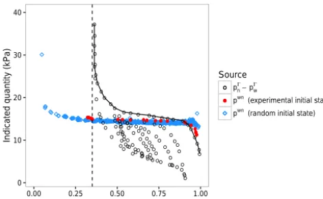
Figure 2. Comparison between the experimentally measured
boundary pressure difference p0n−pw0 and the capillary
pres-sure pwn for the micromodel geometry. The solid line represents
the boundary pressure along primary drainage.
fluids. Based on the final fluid configurations, connectivity-based analysis was performed to infer macroscale capillary pressure, saturation, and interfacial area for a dense set of equilibrium states.
5.3 Results and discussion
Phase connectivity presents a critical challenge for the theory and simulation of two-fluid-phase flow. When all or part of a phase forms a fully connected pathway through a porous medium, flow can occur without the movement of inter-faces. However, the case where phase sub-regions are not connected is a source of history-dependent behavior in tra-ditional models. Tratra-ditional models make use of the capil-lary pressure proposed as a function of the fluid saturation only, pc(sw). However, this relationship is not unique. Fur-thermore, key features of the relationship are an artifact of the experimental design. For example, the irreducible wetting-phase saturation,sIw, can play an important role.
To calculate pw as it is defined from Eq. (5), the mi-croscale pressure field must be known throughout the do-main. Simulation provides a means to study how the pres-sure varies within the system and to obtain averages within all phase sub-regions. Based on Eq. (16), values ofpwi,Jwin
w ,
andwi can be determined for each connected region of the
wetting phasewifori∈ {1, 2, . . . ,Nw}. Two sets of
simula-tions were performed, including (1) a set of 24 configurasimula-tions initialized directly from experimentally observed tions along primary drainage, and (2) a set of 48 configura-tions with random initial condiconfigura-tions as discussed in Sect. 5.2. The equilibrium fluid arrangements were analyzed to deter-mine the true capillary pressure, pwn, by analyzing the cur-vature of the fluid–fluid interface, fluid saturation, sw, and specific interfacial area, wn. The data were aggregated to produce a dense set of equilibrium configurations.
Pressure transducers located in each of the two-fluid reser-voirs were used to measure experimental boundary pressures for each fluid. The resulting values ofpn0−p0w are plotted in Fig. 2. Average capillary pressure values calculated from the simulations are presented along with this experimental data. The solid line represents the boundary pressure differ-ence during primary drainage. The boundary pressures for simulations initialized from experimental data matched the experimentally measured values ofpn0−pw0exactly. Bound-ary measurements taken during simulation are also presented for imbibition and scanning curve sequences. The values of
p0n−p0wplotted in Fig. 2 represent a comprehensive set of experimental measurements that would typically be identi-fied as capillary pressure values. This provides a basis for comparison with measurements of the true capillary pres-sure based on the configuration of the interfaces. In gen-eral, agreement betweenp0n−p0wandpwnshould not be ex-pected. Only when both the w andn fluids are fully con-nected and when the system is at equilibrium will the bound-ary pressure difference balance the internal average capillbound-ary pressure. The difference between the boundary measurement and the internal average capillary pressure due to the phases being disconnected is evident by comparing the experimen-tal data from primary drainage and the simulation points initialized from the associated fluid configurations. Pressure boundary conditions for the simulations were set to match the measured values ofp0n andp0w. Assw decreases, there is an increasing gap betweenpn0−pw0and the average capil-lary pressurepwn. This gap is attributed to the formation of disconnected wetting-phase regions during drainage, an ef-fect that is most significant as the irreducible wetting-phase saturation is approached.
In the experimental system, an irreducible wetting-phase saturation was clearly observed assIw=0.35. This value is marked with a vertical dashed line in Fig. 2. This irreducible wetting-phase saturation corresponds to the lowest experi-mentally accessible wetting-phase saturation, since fluid con-figurations withsw< sIwcannot be obtained from the exper-imental setup and operating conditions. The underlying rea-son for this is related to the connectivity of the wetting phase. This can be understood from Fig. 3, which shows the phase configuration observed experimentally at the end of primary drainage. Within a connected region of wetting phase, the mi-croscale pressure,pw, will tend to be nearly constant.
How-ever, the wetting-phase pressure can vary from one region to another. The connected components of the wetting phase are shown in Fig. 3b. At equilibrium, the measured differ-ence in boundary pressuresp0n−p0wmust balance with the capillary pressure of the interface sub-region between the two-phase components. Note that the non-wetting phase is fully connected in Fig. 3a. The implication is thatpn0=pn
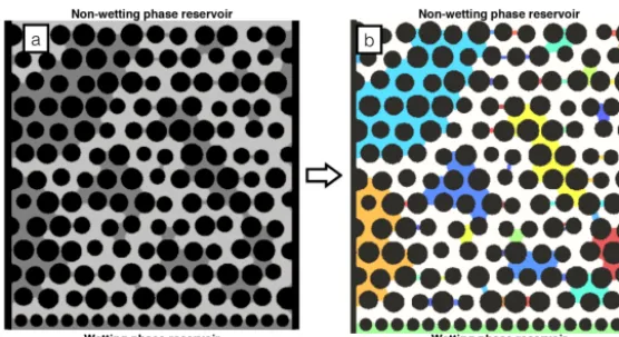
Figure 3.Phase connectivity has a direct impact on the meaning of the macroscale experimental measurements:(a)experimentally observed
phase configuration corresponding to irreducible wetting-phase saturation, and(b)connected components analysis shows all wetting phase
that remains in the system is disconnected from the wetting-phase reservoir. The black denotes the solid phase, the gray and various colors denote the wetting phase, and the white denotes the non-wetting phase.
in Fig. 3b. The part ofw that is connected to the
wetting-phase reservoir is shown in light green in Fig. 3b. When the irreducible wetting-phase saturation is reached the portion ofwthat connects to the reservoir no longer fills any of the
pore space within the micromodel. The irreducible wetting-phase saturation is associated with the trapped wetting-wetting-phase regions only. Changing the pressure difference between the fluid reservoirs to increase p0n−pw0 does not change the capillary pressure in these regions. This leads to arbitrar-ily high measurements, claimed to be “capillary pressure” measurements, which are actually a difference in reservoir pressures rather than a measure of interface curvature. This also misconstrues the reduction in wetting-phase saturation that occurs. The true average capillary pressure, as defined in Eq. (12), is much lower. Furthermore, the wetting-phase saturation can be further reduced as a consequence of other processes, such as evaporation. It is irreducible only within the context of the experimental design.
In light of this result, it is useful to consider alternative means to generate two-fluid configurations in porous me-dia. For example, suppose a fluid configuration was encoun-tered withsw=0.2, a value lower than the irreducible satu-ration. How can we determine the macroscale capillary pres-sure? From a traditional macroscale parameterization ap-proach, the experimentally proposed relationpwn(sw)is of absolutely no use, since capillary pressure is undefined for
sw< swI. From the microscale perspective, it is clearly pos-sible to produce fluid configurations for whichsw< sIw (for any system), and to measure the associated capillary pressure based on Eq. (12). For randomly initialized phase configu-rations, many such systems are produced. Simulations per-formed based on these initial geometries lead to equilibrium capillary pressure measurements shown in Fig. 2. While the classic “J curve” shape is still present, the experimentally determined valuesIwoffers no guidance regarding this form.
Comparing capillary pressures measured from random ini-tial conditions with those measured from experimental iniini-tial conditions provides additional insight. First, the true capil-lary pressure measurements based on Eq. (8) are remarkably consistent, particularly when considering the values ofpwn
obtained assw→swI. Compared to randomly initialized data, configurations from primary drainage have a higher aver-age capillary pressure. This is expected, since along primary drainagepwn is determined by the pore-throat sizes. These represent the highest capillary pressures that are typically ob-served. We note that primary drainage does not specify the maximum possible capillary pressure, since bubbles of non-wetting phase may form that have a smaller radius of curva-ture than the minimum throat width.
Figure 4.Contour plot showing the relationshippwn(sw,wn), with contours showing the capillary pressurepwn(kPa). Data points used to construct the surface are also shown, including randomly initial-ized fluid configurations and experimentally initialinitial-ized configura-tions from primary drainage.
random and experimentally observed initial conditions. The black lines in Fig. 4 show the iso-contours of the capillary pressure surface. It is clear that primary drainage leads to states with lower interfacial area as compared to randomly initialized configurations. Both sets of points lie along a con-sistent surface. The extent to which the relationshipspwn(sw)
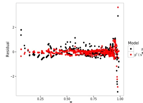
and pwn(sw, wn) describe the data points measured from microscale configurations is quantitatively assessed by eval-uating the residuals for the GAM approximation. The resid-uals are shown in Fig. 5. The traditionally used relationship
pwn(sw)is able to explain only 60.6 % of the variance in the data. When the effect of interfacial area is included,pwn(sw,
wn), 77.1 % of the variance is explained. Based on previous work for three-dimensional porous media, it is anticipated that higher fidelity approximations can be produced by in-cluding the effects of other topological invariants, such as the average Gaussian curvature or the Euler characteristic (Mc-Clure et al., 2016b).
6 Conclusions
In this work, we show that the ability to quantitatively ana-lyze the internal structure of two-fluid porous medium sys-tems has a profound impact on macroscale understanding. We considered the behavior of the capillary pressure based on traditional laboratory boundary measurements and com-pare this to the true average capillary pressure, a state func-tion, determined by directly averaging the curvature of the interface between fluids. We demonstrate that the difference between the phase pressures as measured from the boundary cannot be used to deduce the capillary pressure of the sys-tem. In particular, the high capillary pressure measured for
● ● ● ● ● ● ● ● ● ● ● ● ● ● ● ● ● ● ● ● ● ● ● ● ● ● ● ● ● ● ● ● ● ● ● ● ● ● ● ● ● ● ● ● ● ● ● ● ● ● ● ● ● ● ● ● ● ● ● ● ● ● ● ● ● ● ● ● ● ● ● ● ● ● ● ● ● ● ● ● ● ● ● ● ● ● ● ● ● ● ● ● ● ● ● ● ● ● ● ● ● ● ● ● ● ● ● ● ● ● ● ● ● ● ● ● ● ● ● ● ● ● ● ● ● ● ● ● ● ● ● ● ● ● ● ● ● ● ● ● ● ● ● ● ● ● ● ● ● ● ● ● ● ● ● ● ● ● ● ● ● ● ● ● ● ● ● ● ● ● ● ● ● ● ● ● ● ● ● ● ● ● ● ● ● ● ● ● ● ● ● ● ● ● ● ● ● ● ● ● ● ● ● ● ● ● ● ● ● ● ● ● ● ● ● ● ● ● ● ● ● ● ● ● ● ● ● ● ● ● ● ● ● ● ● ● ● ● ● ● ● ● ● ● ● ● ● ● ● ● ● ● ● ● ● ● ● ● ● ● ● ● ● ● ● ● ● ● ● ● ● ● ● ● ● ● ● ● ● ● ● ● ● ● ● ● ● ● ● ● ● ● ● ● ● ● ● ● ● ● ● ● ● ● ● ● ● ● ● ● ● ● ● ● ● ● ● ● ● ● ● ● ● ● ● ● ● ● ● ● ● ● ● ● ● ● ● ● ● ● ● ● ● ● ● ● ● ● ● ● ● ● ● ● ● ● ● ● ● ● ● ● ● ● ● ● ● ● ● ● ● ● ● ● ● ● ● ● ● ● ● ● ● ● ● ● ● ● ● ● ● ● ● ● ● ● ● ● ● ● ● ● ● ● ● ● ● ● ● ● ● ● ● ● ● ● ● ● ● ● ● ● ● ● ● ● ● ● ● ● ● ● ● ● ●●●●●●●●●●●●● ● ● ● ● ● ● ● ● ● ● ●●●●●●●●●●●● ● ● ● ● ● ● ● ● ● ● ● ● ●●●●●●●●●●●● ●●●●●●●● ● ● ● ● ● ● ● ●●●●●●●●●●● ●● ● ● ● ● ● ● ● ● ● ● ● ● ● ● ● ● ● ● ● ● ● ● ● ● ● ● ● ● ● ● ● ● ● ● ● ● ●● ● ● ● ● ● ● ● ● ● ● ● ● ● ● ● ● ● ● ● ● ● ● ● ● ● ● ● ● ● ● ● ● ● ● ● ● ● ● ● ● ● ● ● ● ● ● ● ● ● ● ● ● ● ● ● ● ● ● ● ● ● ● ● ● ● ● ● ● ● ● ● ● ● ● ● ● ● ● ● ● ● ● ● ● ● ● ● ● ● ● ● ● ● ● ● ● ● ● ● ● ● ● ● ● ● ● ● ● ● ● ● ● ● ● ● ● ● ● ● ● ● ● ● ● ● ● ● ● ● ● ● ● ● ● ● ● ● ● ● ● ● ● ● ● ● ● ● ● ● ● ● ● ● ● ● ● ● ● ● ● ● ● ● ● ● ● ● ● ● ● ● ● ● ● ● ● ● ● ● ● ● ● ● ● ● ● ● ● ● ● ● ● ● ● ● ● ● ● ● ● ● ● ● ● ● ● ● ● ● ● ● ● ● ● ● ● ● ● ● ● ● ● ● ● ● ● ● ● ● ● ● ● ● ● ● ● ● ● ● ● ● ● ● ● ● ● ● ● ● ● ● ● ● ● ● ● ● ● ● ● ● ● ● ● ● ● ● ● ● ● ● ● ● ● ● ● ● ● ● ● ● ● ● ● ● ● ● ● ● ● ● ● ● ● ● ● ● ● ● ● ● ● ● ● ● ● ● ● ● ● ● ● ● ● ● ● ● ● ● ● ● ● ● ● ● ● ● ● ● ● ● ● ● ● ● ● ● ● ● ● ● ● ● ● ● ● ● ● ● ● ● ● ● ● ● ● ● ● ● ● ● ● ● ● ● ● ● ● ● ● ● ● ● ●●●● ● ● ● ● ● ● ● ● ● ● ● ● ● ● ● ● ● ● ● ● ● ● ● ● ● ● ● ● ● ● ● ● ● ● ● ● ● ● ● ● ● ● ● ● ● ● ● ● ● ● ● ● ● ● ● ● ● ● ● ● ● ● ● ● ● ● ● ● ● ● ● ● ● ● ● ● ● ● ● ● ● ● ● ● ●●●●●●●●●●●●●●●●●●●●●●● ● ● ● ● ● ● ● ● ● ● ● ● ● ● ● ● ● ● ● ● ● ● ● ● ● ● ● ● ● ● ● ● ● ● ● ● ● ● ● ● ● ● ● ● ● ● ● ● ● ● ● ●●●●●●●●●●● ●● ● ● ● ● ● ● ● ● ● ● ● ● ● ● ● ● ● ● ● ● ● ● ● ● ● ● ●●● ● ● ● ● ● ● ● ● ● ● ● ● ● ● ● ● ● ● ● ● ● ● ● ● ● ● ● ● ● ● ● ● ● ● ● ● −2 0 2
0.25 0.50 0.75 1.00
sw Residual Model ● ● ● ●
pc(sw)
[image:11.612.47.283.66.228.2]pc(sw, εwn)
Figure 5.Comparison of the residual errors for the GAM fits that
approximatepwn(sw)andpwn(sw,wn).
irreducible wetting-phase saturation is an artifact of the ex-perimental design. Three important conclusions result.
First, the true capillary pressure measured at tradition-ally identified irreducible wetting-phase saturation is signif-icantly lower than predicted from boundary pressure mea-surements. This can be understood based on the underlying phase connectivity. At irreducible wetting-phase saturation, the wetting-phase reservoir pressure no longer reflects the internal pressure of the system since the reservoir does not connect to the remaining wetting phase inside the system.
Second, randomly generated fluid configurations provide a way to access states where the wetting-phase saturation is be-low the irreducible wetting-phase saturation. By carrying out direct averaging based on these states, the capillary pressure state function can be computed over the full range of possi-ble saturation values, including configurations that are inac-cessible from traditional experiments. We note that modified experimental designs could be used to accomplish the same studies.
7 Data availability
Data associated with this publication have been made pub-licly available on the Digital Rock Portal (https://www. digitalrocksportal.org/projects/84/). This data set includes the experimentally observed fluid configurations within the micromodel systems as well as a complete log of the compu-tationally generated equilibrium configurations. The DOI for the data set is doi:10.17612/P74S31.
Author contributions. All authors participated in the writing of this manuscript. William G. Gray and Cass T. Miller contributed to the introduction, background, and theory, Amanda L. Dye contributed to the microfluidics, and James E. McClure contributed to lattice Boltzmann modeling. All authors contributed to the discussion and conclusions from this work.
Competing interests. The authors declare that they have no conflict of interest.
Acknowledgements. This work was supported by Army
Re-search Office grant W911NF-14-1-02877, Department of
Energy grant DE-SC0002163, and National Science Foundation grant 1619767. An award of computer time was provided by the Department of Energy INCITE program. This research also used resources of the Oak Ridge Leadership Computing Facility, which is a DOE Office of Science User Facility supported under contract DE-AC05-00OR22725.
Edited by: R. Uijlenhoet
Reviewed by: two anonymous referees
References
Albers, B.: Modeling the hysteretic behavior of the capillary pres-sure in partially saturated porous media: a review, Acta Mechan-ica, 225, 2163–2189, 2014.
Alizadeh, A. H. and Piri, M.: The effect of saturation history on three-phase relative permeability: An experimental study, Water Resour. Res., 50, 1636–1664, 2014.
Anderson, T. B. and Jackson, R.: A fluid mechanical description of fluidized beds, Indust. Eng. Chem. Fundament., 6, 527–539, 1967.
Bachmat, Y. and Bear, J.: The General Equations of Hydrodynamic Dispersion in Homogeneous, Isotropic, Porous Mediums, J. Geo-phys. Res., 69, 2561–2567, 1964.
Bauer, P., Thorpe, A., and Brunet, G.: The quiet revolution of nu-merical weather prediction, Nature, 525, 47–55, 2015.
Bear, J.: Dynamics of Fluids in Porous Media, Elsevier, New York, 1972.
Bernard, P. S. and Wallace, J. M.: Turbulent Flow, John Wi-ley & Sons, Hoboken, New Jersey, USA, 2002.
Blöschl, G.: Scaling in Hydrology, Hydrol. Process., 15, 709–711, 2001.
Blöschl, G., Grayson, R. B., and Sivapalan, M.: On the representa-tive elementary area (rea) concept and its utility for distributed rainfall-runoff modelling, Hydrol. Process., 9, 313–330, 1995. Bradshaw, P.: An Introduction to Turbulence and its Measurement,
Pergamon Press, Elmsford, New York, USA, 1971.
Chanson, H.: Current knowledge in hydraulic jumps and related phenomena. A survey of experimental results, Eur. J. Mech. B Fluids, 28, 191–210, 2009.
Collins, R., Triplett, C., Barjatya, A., Lehmacher, G., and Fritts, D.: Using lidar and rockets to explore turbulence in the atmosphere, SPIE Newsroom, doi:10.1117/2.1201505.005922, 2015. Cushman, J. H.: The Physics of Fluids in Hierarchical Porous
Me-dia: Angstroms to Miles, Kluwer Academic Publishers, Dor-drecht, the Netherlands, 1997.
D’Asaro, E. A.: Turbulence in the Upper-Ocean Mixed Layer, Ann. Rev. Mar. Sci., 6, 101–115, 2014.
Deems, J. S., Painter, T. H., and Finnegan, D. C.: Lidar measure-ment of snow depth: a review, J. Glaciol., 59, 467–479, 2013. Dietrich, J. C., Dawson, C. N., Proft, J. M., Howard, M. T., Wells,
G., Fleming, J. G., Luettich Jr., R. A., Westerink, J. J., Cobell, Z., Vitse, M., Lander, H., Blanton, B. O., Szpilka, C. M., and Atkin-son, J. H.: Real-time forecasting and visualization of hurricane
waves and storm surges using SWAN+ADCIRC and FigureGen,
in: Computational Challenges in the Geosciences, vol. 156 of The IMA Volumes in Mathematics and Its Applications, edited by: Dawson, C. and Gerritsen, M., Springer Science & Business Media, New York, 2013.
Dudhia, J.: A history of mesoscale model development, Asia-Pacific J. Atmos. Sci., 50, 121–131, 2014.
Dye, A. L., McClure, J. E., Gray, W. G., and Miller, C. T.: Multi-scale modeling of porous medium systems, in: chap. 1, 3rd Edn., Handbook of Porous Media, edited by: Vafai, K., CRC Press, Boca Raton, Florida, USA, 3–45, 2015.
Essex, C., McKitrick, R., and Andresen, B.: Does a Global Temper-ature Exist?, J. Non-Equilib. Thermodyn., 32, 1–27, 2007. Flint, L. E., Flint, A. L., Thorne, J. H., and Boynton, R.:
Fine-scale hydrologic modeling for regional landscape application: the California Basin characterization model development and perfor-mance, Ecol. Process., 2, doi:10.1186/2192-1709-2-25, 2013. Fuentes, F. C., Iungo, G. V., and Porté-Agel, F.: 3D turbulence
measurements using three synchronous wind lidars: Validation against sonic anemometry, J. Atmos. Ocean. Tech., 31, 1549– 1556, 2014.
Gentine, P., Troy, T. J., Lintner, B. R., and Findell, K. L.: Scaling in Surface Hydrology: Progress and Challenges, J. Contemp. Water Res. Educ., 147, 28–40, 2012.
Gleeson, T. and Paszkowski, D.: Perceptions of scale in hydrology: What do you mean by regional scale?, Hydrolog. Sci. J., 59, 99– 107, doi:10.1080/02626667.2013.797581, 2014.
Gray, W. G. and Miller, C. T.: Thermodynamically constrained averaging theory approach for modeling flow and trans-port phenomena in porous medium systems: 7. Single-phase megascale flow models, Adv. Water Resour., 32, 1121–1142, doi:10.1016/j.advwatres.2009.05.010, 2009.
Gray, W. G. and Miller, C. T.: Introduction to the Thermodynami-cally Constrained Averaging Theory for Porous Media Systems, Springer-Verlag, New York, USA, 2014.
Gray, W. G. and O’Neill, K.: On the development of Darcy’s law for the general equations for flow in porous media, Water Resour. Res., 12, 148–154, 1976.
Gray, W. G., Dye, A. L., McClure, J. E., Pyrak-Nolte, L. J., and Miller, C. T.: On the dynamics and kinematics of two-fluid-phase flow in porous media, Water Resour. Res., 51, 5365–5381, 2015. Hermann, S. M. and Sop, T. K.: The map is not the territory: How satellite remote sensing and ground evidence have re-shaped the image of Sahelian desertification, in: The End of Desertifica-tion? Disputing Enviornmental Change in the Drylands, Springer Earth System Sciences, edited by: Behnke, R. and Mortimore, M., Springer, New York, USA, 117–145, 2016.
Hornung, U.: Homogenization and Porous Media, in: no. 6 in In-terdisciplinary Applied Mathematics, Springer, New York, USA, 1997.
Ishii, M., Kim, S., and Kelly, J.: Development of Interfacial Area Transport Equation, Nucl. Eng. Technol., 37, 525–536, 2005. Kauffeldt, A., Halldin, S., Rodhe, A., Xu, C.-Y., and Westerberg,
I. K.: Disinformative data in large-scale hydrological modelling, Hydrol. Earth Syst. Sci., 17, 2845–2857, doi:10.5194/hess-17-2845-2013, 2013.
Kauffeldt, A., Wetterhall, F., Pappenberger, F., Salamon, P., and Thielen, J.: Technical review of large-scale hydrological mod-els for implementation in operational flood forecasting schemes on continental level, Environ. Model. Softw., 75, 68–76, 2016. Knödel, K., Lange, G., and Voigt, H.-J.: Environmental Geology:
Handbook of Field Methods and Case Studies, Springer, Berlin, Heidelberg, New York, 2007.
Kocamustafaogullari, G. and Ishii, M.: Foundation of the interfacial area transport equation and its closure relations, Int. J. Heat Mass Trans., 38, 481–493, 1995.
Lillesand, T. M., Kiefer, R. W., and Chipman, J. W.: Remote Sens-ing and Image Interpretation, 7th Edn., Wiley, Hoboken, New Jersey, USA, 2015.
Ly, S., Charles, C., and Degré, A.: Different methods for spatial interpolation of rainfall data for operational hydrology and hy-drological modeling at watershed scale. A review, Biotechnol. Agron. Soc. Environ., 17, 392–406, 2013.
Marle, C.: Ècoulements monophasiques en milieu poreux, Revue de L’Institut Français du Pétrole, 22, 1471–1509, 1967.
Maugin, G. A.: The Thermomechanics of Nonlinear Irreversible Behaviors: An Introduction, World Scientific Press, Singapore, 1999.
McClure, J. E., Prins, J. F., and Miller, C. T.: A Novel Heteroge-neous Algorithm to Simulate Multiphase Flow in Porous Me-dia on Multicore CPU-GPU Systems, Comput. Phys. Commun., 185, 1865–1874, doi:10.1016/j.cpc.2014.03.012, 2014a. McClure, J. E., Wang, H., Prins, J. F., Miller, C. T., and Feng, W.:
Petascale Application of a Coupled CPU-GPU Algorithm for Simulation and Analysis of Multiphase Flow Solutions in Porous Medium Systems, in: 28th IEEE International Parallel & Dis-tributed Processing Symposium, Phoenix, Arizona, 2014b. McClure, J. E., Berrill, M. A., Gray, W. G. and Miller, C. T.:
Track-ing Interface and Common Curve Dynamics for Two-Fluid Flow in Porous Media, J. Fluid Mech., 796, 211–232, 2016a.
McClure, J. E., Berrill, M. A., Gray, W. G. and Miller, C. T.: In-fluence of phase connectivity on the relationship among cap-illary pressure, fluid saturation, and interfacial area in two-fluid-phase porous medium systems, Phys. Rev. E, 94, 033102, doi:10.1103/PhysRevE.94.033102, 2016b.
Miller, C. T., Christakos, G., Imhoff, P. T., McBride, J. F., Pedit, J. A., and Trangenstein, J. A.: Multiphase flow and transport modeling in heterogeneous porous media: Challenges and ap-proaches, Adv. Water Resour., 21, 77–120, 1998.
Miller, C. T., Dawson, C. N., Farthing, M. W., Hou, T. Y., Huang, J. F., Kees, C. E., Kelley, C. T., and Langtangen, H. P.: Numerical simulation of water resources problems: Mod-els, methods, and trends, Adv. Water Resour., 51, 405–437, doi:10.1016/j.advwatres.2012.05.008, 2013.
Nickerson, C., Ebel, R., Borchers, A., and Carriazo, F.: Major Uses of Land in the United States, 2007, EIB-89, US Department of Agriculture, Economic Research Service, December 2011. Niessner, J., Berg, S., and Hassanizadeh, S. M.:
Compari-son of Two-Phase Darcy’s Law with a Thermodynamically Consistent Approach, Transport Porous Media, 88, 133–148, doi:10.1007/s11242-011-9730-0, 2011.
Paiva, R. C. D., Collischonn, W., and Tucci, C. E. M.: Large scale hydrologic and hydrodynamic modeling using limited data and a GIS based approach, J. Hydrol., 406, 170–181, 2011.
Panfilov, M.: Macroscale Models of Flow Through Highly Het-erogeneous Porous Media, Springer, Dordrecht, the Netherlands, 2000.
Pechlivanidis, I. G., Jackson, B. M., McIntyre, N. R., and Wheater, H. S.: Catchment scale hydrological modelling: A review of model types, calibration approaches and uncertainty analysis methods in the context of recent developments in technology and applications, Global NEST J., 13, 193–214, 2011.
Reggiani, P., Sivapalan, M., and Hassanizadeh, S. M.: A Unifying Framework for Watershed Thermodynamics: Balance Equations for Mass, Momentum, Energy and Entropy, and the Second Law of Thermodynamics, Adv. Water Resour., 22, 367–398, 1998. Reggiani, P., Hassanizadeh, S. M., Sivapalan, M., and Gray, W. G.:
A Unifying Framework for Watershed Thermodynamics: Consti-tutive Relationships, Adv. Water Resour., 23, 15–39, 1999. Sathe, A. and Mann, J.: A review of turbulence measurements using
ground-based wind lidars, Atmos. Meas. Tech., 6, 3147–3167, doi:10.5194/amt-6-3147-2013, 2013.
Skøien, J. O., Blöschl, G., and Western, A. W.: Characteristic space scales and timescales in hydrology, Water Resour. Res., 39, 11-1–11-19, 2003.
Vreugdenhil, C. B.: Numerical Methods for Shallow-Water Flow, in: no. 13 in Water Science and Technology Library, Springer, Dordrecht, the Netherlands, 1995.
Wang, A., Zeng, X., Shen, S. S. P., Zeng, Q.-C., and Dickinson, R. E.: Time Scales of Land Surface Hydrology, J. Hydrometeorol., 7, 868–879, 2006.
Whitaker, S.: Diffusion and Dispersion in Porous Media, Am. Inst. Chem. Eng. J., 13, 420–427, 1967.
Whitaker, S.: Flow in Porous Media I: A Theoretical Derivation of Darcy’s Law, Transport Porous Media, 1, 3–25, 1986.
Whitaker, S.: The Method of Volume Averaging, Kluwer Academic Publishers, Dordrecht, 1999.
in subsurface porous medium systems, Adv. Water Resour., 51, 217–246, 2013.
Wood, E. F.: Scaling behaviour of hydrological fluxes and variables: Empirical studies using a hydrological model and remote sensing data, Hydrol. Process., 9, 331–346, 1995.
Wood, E. F., Sivapalan, M., Beven, K., and Band, L.: Effects of spa-tial variability and scale with implications to hydrologic model-ing, J. Hydrol., 102, 29–47, 1988.
Wood, S. N.: Fast stable direct fitting and smoothness selection for generalized additive models, J. Roy. Stat. Soc. Ser. B, 70, 495– 518, 2008.