Examining the validity and reliability of the Activities Specific Balance Confidence Scale 6 (ABC 6) in a diverse group of older adults

ScholarWorks @ Georgia State University

ScholarWorks @ Georgia State University

Risk Management and Insurance Dissertations Department of Risk Management and Insurance

8-7-2012

Essays on Lifetime Uncertainty: Models, Applications, and

Essays on Lifetime Uncertainty: Models, Applications, and

Economic Implications

Economic Implications

Nan Zhu

Georgia State University

Follow this and additional works at: https://scholarworks.gsu.edu/rmi_diss

Recommended Citation Recommended Citation

Zhu, Nan, "Essays on Lifetime Uncertainty: Models, Applications, and Economic Implications." Dissertation, Georgia State University, 2012.

https://scholarworks.gsu.edu/rmi_diss/30

PERMISSION TO BORROW

In presenting this dissertation as a partial fulfillment of the requirements for an advanced

degree from Georgia State University, I agree that the Library of the University shall make it

available for inspection and circulation in accordance with its regulations governing materials

of this type. I agree that permission to quote from, to copy from, or publish this dissertation

may be granted by the author or, in his/her absence, the professor under whose direction

it was written or, in his absence, by the Dean of the Robinson College of Business. Such

quoting, copying, or publishing must be solely for the scholarly purposes and does not

involve potential financial gain. It is understood that any copying from or publication of

this dissertation which involves potential gain will not be allowed without written permission

of the author.

All dissertations deposited in the Georgia State University Library must be used only in

accordance with the stipulations prescribed by the author in the preceding statement.

The author of this dissertation is:

Nan Zhu

35 Broad Street NW, 11th Floor, Atlanta, GA 30303

The director of this dissertation is:

Daniel Bauer

Department of Risk Management and Insurance

Essays on Lifetime Uncertainty: Models, Applications, and Economic Implications

BY

Nan Zhu

A Dissertation Submitted in Partial Fulfillment of the Requirements for the Degree

Of

Doctor of Philosophy

In the Robinson College of Business

Of

Georgia State University

GEORGIA STATE UNIVERSITY

ROBINSON COLLEGE OF BUSINESS

Nan Zhu

ACCEPTANCE

This dissertation was prepared under the direction of the Nan Zhu Dissertation

Commit-tee. It has been approved and accepted by all members of that committee, and it has been

accepted in partial fulfillment of the requirements for the degree of Doctoral of Philosophy

in Business Administration in the J. Mack Robinson College of Business of Georgia State

University.

H. Fenwick Huss, Dean

DISSERTATION COMMITTEE

Daniel Bauer

Conrad S. Ciccotello

Shiferaw Gurmu

Richard D. Phillips

Essays on Lifetime Uncertainty: Models, Applications, and Economic Implications

BY

Nan Zhu

July 11, 2012

Committee Chair: Daniel Bauer

Major Academic Unit: Department of Risk Management and Insurance

My doctoral thesis “Essays on Lifetime Uncertainty: Models, Applications, and Eco-nomic Implications” addresses economic and mathematical aspects pertaining to uncertain-ties in human lifetimes. More precisely, I commence my research related to life insurance markets in a methodological direction by considering the question of how to forecast aggre-gate human mortality when risks in the resulting projections is important. I then rely on the developed method to study relevant applied actuarial problems. In a second strand of research, I consider the uncertainty in individual lifetimes and its influence on secondary life insurance market transactions.

My first essay “Coherent Modeling of the Risk in Mortality Projections: A Semi-Parametric Approach” deals with stochastically forecasting mortality. In contrast to previous approaches, I present the first data-driven method that focuses attention on uncertainties in mortality projections rather than uncertainties in realized mortality rates. Specifically, I analyze time series of mortality forecasts generated from arbitrary but fixed forecasting methodologies and historic mortality data sets. Building on the financial literature on term structure mod-eling, I adopt a semi-parametric representation that encompasses all models with transitions parameterized by a Normal distributed random vector to identify and estimate suitable spec-ifications. I find that one to two random factors appear sufficient to capture most of the variation within all of our data sets. Moreover, I observe similar systematic shapes for their volatility components, despite stemming from different forecasting methods and/or different mortality data sets. I further propose and estimate a model variant that guarantees a non-negative process of the spot force of mortality. Hence, the resultingforward mortality factor modelspresent parsimonious and tractable alternatives to the popular methods in situations where the appraisal of risks within medium or long-term mortality projections plays a dom-inant role.

Relying on a simple version of the derived forward mortality factor models, I take a closer look at their applications in the actuarial context in the second essay “Applications of Forward Mortality Factor Models in Life Insurance Practice.”1 In the first application, I derive the Economic Capital for a stylized UK life insurance company offering traditional product lines. My numerical results illustrate that (systematic) mortality risk plays an important role for a life insurer’s solvency. In the second application, I discuss the valuation of different common mortality-contingent embedded options within life insurance contracts. Specifically, I present a closed-form valuation formula forGuaranteed Annuity Optionswithin traditional endowment policies, and I demonstrate how to derive the fair option fee for a

Guaranteed Minimum Income Benefit within a Variable Annuity Contract based on Monte Carlo simulations. Overall my results exhibit the advantages of forward mortality factor models in terms of their simplicity and compatibility with classical life contingencies theory.

The second major part of my doctoral thesis concerns the so-calledlife settlement mar-ket, i.e. the secondary market for life insurance policies. Evolving from so-called “viatical settlements” popular in the late 1980s that targeted severely ill life insurance policyholders, life settlements generally involve senior insureds with below average life expectancies. Within such a transaction, both the liability of future contingent premiums and the benefits of a life insurance contract are transferred from the policyholder to a life settlement company, which may further securitize a bundle of these contracts in the capital market.

One interesting and puzzling observation is that although life settlements are advertised as a high-return investment with a low “Beta”, the actual market systematically underper-formed relative to expectations. While the common explanation in the literature for this gap between anticipated and realized returns falls on the allegedly meager quality of the underlying life expectancy estimates, my third essay “Coherent Pricing of Life Settlements

cyholders’ health states is asymmetric, my model shows that a discrepancy naturally arises in a competitive market when the decision to settle is taken into account for pricing the life settlement transaction, since the life settlement company needs to shift its pricing schedule in order to balance expected profits. I derive practically applicable pricing formulas that account for the policyholder’s decision to settle, and my numerical results reconfirm that— depending on the parameter choices—the impact of asymmetric information on pricing may be considerable. Hence, my results reveal a new angle on the financial analysis of life settle-ments due to asymmetric information.

ix

DEDICATION

ACKNOWLEDGEMENTS

I owe my advisor, Professor Daniel Bauer greatly, for his most patient, insightful, and encouraging guidance throughout my Ph.D. study. Without him I could never have finished this work. I would also like to thank my committee members, Professors Conrad Ciccotello, Shiferaw Gurmu, Richard Phillips, and Ajay Subramanian for their instructive suggestions. In particular, my gratitude goes to Professor Richard Phillips and Professor Ajay Subra-manian for their continuous encouragements for my research and generous funding for my conference presentations.

Best wishes to my Ph.D. fellows, Jin Gao, Hae Won Jung, Fan Liu, Jimmy Martinez, Thorsten Moenig, and Xue Qi for all the laughters and tears we shared over the years. With-out you folks I could not recognize the Department of Risk Management and Insurance at Georgia State University as my second home.

xi

TABLE OF CONTENTS

DEDICATION . . . ix

ACKNOWLEDGEMENTS . . . x

LIST OF FIGURES . . . xiv

LIST OF TABLES . . . xv

Chapter 1 COHERENT MODELING OF THE RISK IN MORTALITY PROJECTIONS: A SEMI-PARAMETRIC APPROACH xvii 1.1 Introduction . . . xvii

1.2 A Factor Model of Mortality Forecasts . . . xxv

1.2.1 Mortality Forecasts . . . xxv

1.2.2 Data . . . xxix

1.2.3 Factor Analysis . . . xxxii

1.2.4 Simple Factor Models . . . xl

1.3 Forward Mortality Factor Models . . . xlv

1.3.1 Theory . . . xlv

1.3.2 Econometrical Approach . . . xlvii

1.3.3 Maximum Likelihood Estimation . . . liv

1.4 A Non-negative Model Variant . . . lxiv

1.5 Application . . . lxvii

1.6 Conclusion . . . lxx

1.7 Appendix: Proofs . . . lxxii

Chapter 2 APPLICATIONS OF FORWARD MORTALITY FACTOR

MODELS IN LIFE INSURANCE PRACTICE . . . . lxxiv

2.1 Introduction . . . lxxiv

2.2 Forward Mortality Factor Models . . . lxxvii

2.3 Application I: Economic Capital in Internal Models . . . lxxxiii

2.3.1 Model Framework . . . lxxxiii

2.3.2 A Stylized Life Insurance Company . . . lxxxvi

2.3.3 Implementation . . . lxxxviii

2.3.4 Results . . . xciii

2.4 Application II: Valuation of Annuitization Options . . . xcvii

2.4.1 Valuation of Guaranteed Annuity Options . . . xcvii

2.4.2 Valuation of Guaranteed Minimum Income Benefits . . . cii

2.4.3 Implementation and Results . . . ciii

2.5 Conclusion . . . cvii

2.6 Appendix: Principle Component Analysis . . . cviii

xiii

3.1 Introduction . . . cxi

3.2 One-Period Model for Life Settlements . . . cxiv

3.2.1 Symmetric Information . . . cxv

3.2.2 Asymmetric Information . . . cxvi

3.3 The Extended Framework . . . cxxi

3.3.1 Heterogenous Generation Life Tables . . . cxxi

3.3.2 Evaluation of the Policyholder’s Decision . . . cxxiii

3.3.3 Coherent Pricing Formulas . . . cxxiv

3.3.4 Generalization . . . cxxv

3.4 Application . . . cxxvii

3.4.1 Projections of Population/Individual Generation Life Tables . . . cxxvii

3.4.2 Settlement Decision and Derivation of Offer Prices . . . cxxx

3.5 Conclusion . . . cxxxv

LIST OF FIGURES

Figure 1.1 Examples of P-spline Projections, female US data . . . xxxi

Figure 1.2 Eigenvectors for the ENW data, Lee-Carter model . . . xxxv

Figure 1.3 Eigenvectors for the ENW data, CBD-Perks Model . . . xxxviii

Figure 1.4 Eigenvectors for the ENW data, P-spline method . . . xlii

Figure 1.5 Fitting C1(x) with Logistic-Gompertz function, USA data . . . . lii

Figure 1.6 Fitting C2(x) with Logistic-Gompertz function, male population,

Lee-Carter method . . . liv

Figure 1.7 Simulated Life Expectancy After One Year . . . lxix

Figure 2.1 Principal Component Analysis, Estimation, and Projection . . . . lxxxii

Figure 2.2 Empirical CDF of Economic Capital . . . xciv

Figure 3.1 Population Survival Probabilities Projected from the Lee-Carter Method cxxviii

Figure 3.2 Empirical CDFs of Individual Survival Probabilities . . . cxxix

Figure 3.3 Equilibriums under Symmetric Information . . . cxxxi

Figure 3.4 Asymmetric Behavior of Policyholders . . . cxxxii

xv

LIST OF TABLES

Table 1.1 The Six Largest Eigenvalues: Lee-Carter Model . . . xxxvi

Table 1.2 The Six Largest Eigenvalues: CBD-Perks Model . . . xxxix

Table 1.3 The Six Largest Eigenvalues: P-spline Method . . . xli

Table 1.4 Tests for i.i.d. and Normality . . . xliv

Table 1.5 Sample Means and Standard Variances . . . xliv

Table 1.6 The MLE results for female population – Lee-Carter Model . . . . lvii

Table 1.7 The MLE results for male population – Lee-Carter Model . . . lviii

Table 1.8 The MLE results for female population – CBD-Perks Model . . . lviii

Table 1.9 The MLE results for male population – CBD-Perks Model . . . . lix

Table 1.10 The MLE results for female population – P-spline Model . . . lix

Table 1.11 The MLE results for male population –P-spline Model . . . lix

Table 1.12 MLE without Self-Consistency Condition . . . lxiii

Table 1.13 Comparison of Mean and Standard Variance . . . lxiii

Table 1.14 Non-negative estimation: U.S. female & Lee-Carter . . . lxvii

Table 2.2 Estimated capital market parameters . . . lxxxix

Table 2.3 Portfolio for the company, E = 2,000,000 . . . xciv

Table 2.4 Economic capital for the stylized company based on different risk

mea-sures . . . xcv

Table 2.5 Calculations of VaR99% . . . xcvi

Table 2.6 Valuation of GAOs . . . cv

xvii

Chapter 1

COHERENT MODELING OF THE RISK IN MORTALITY PROJECTIONS: A SEMI-PARAMETRIC APPROACH

1.1 Introduction

Having appropriate estimates for the risk in mortality projections is important in many

respects. For instance, a retiree’s personal financial planning decisions will be affected by

his longevity prospects as well as associated uncertainties. For life insurers, pension plans,

and other similar institutions, the risk in mortality projections directly translates into risk

in their liabilities. And even for governments, the extent and the organization of

inter-generational risk sharing depend on the riskiness of aggregate mortality trends. However,

while there exist a growing number of scientific papers on forecasting human mortality, these

contributions have bestowed little attention upon the uncertainty associated with the

result-ing projections. More specifically, the ubiquitous approach relies on past mortality data to furnish a projection of the mortality experience for subsequent periods—possibly involving error terms—that matches the past observations in some optimal sense. In this paper, we

take a different approach by directly focusing on the risk in projections: Given a forecasting methodology, we assess the inherent risks by analyzing time series of forecasts generated

based on a rolling window of annual mortality data, and—in doing so—develop suitable

Clearly, the two approaches are theoretically equivalent since a stochastic model for

mortality experience in every period implies a stochastic mortality forecast and vice versa.

However, the distinction is relevant for the econometrical approach and, therefore, is

impor-tant for the specification and estimation process. This is widely recognized for interest rate

models: There, specifying the short rate is equivalent to specifying models for the entire term

structure of interest rates; yet any meaningful empirical approach requires the consideration

of the entire yield curve data and not only observations on the short end. In particular,

the cross-sectional view is important to identify the persistence and transiency of different

random sources.

Hence, in brief the goal of this paper is to carry over conventional approaches and

techniques for specifying and estimating term structure models to the mortality context and

to apply the resulting models. However, there are some profound differences to interest rate

modeling. First, in addition to the “term”-dimension, there is an “age”-dimension to be taken

into account, and the two enter the relevant equations dissimilarly. Moreover, insurance

prices—from which risk-adjusted mortality projections could potentially be stripped—are

obfuscated by insurance expenses, idiosyncrasies of the particular insured population, and/or

credit risk. Generational life tables, which serve as the actuarial basis for pricing the policies,

on the other hand, are compiled infrequently and come with potential inconsistencies in the

data or the compilation process over time.

As a resolution to the latter point, we base our considerations on mortality forecasts

that are generated from different windows of past mortality experience for ten different

xix

yet very different—forecasting approaches that underlie the compilation of most existing

generational life tables: (1) The Lee-Carter approach (Lee and Carter (1992)), (2) the

CBD-Perks model (Cairns et al. (2006b)), and (3) theP-spline method (Currie et al. (2004)). It is

important to note, however, that we do not adopt the assumptions on the forecasting errors

associated with the approaches but view them as methodologies to generate (deterministic)

forecasts. Therefore, our approach may be interpreted as an attempt to devise a “stochastic

wrap” around existing mortality forecasting approaches that captures the risk in the resulting

projections in a coherent manner.

We are thus given a time series of mortality forecasts in the form of expected survival

probabilities as objects on some space of functions in two variables, namely (current) age

and (forecasting) time horizon. Dynamic stochastic models can then be formulated via a

stochastic (differential) equation in this function space. By initially restricting ourselves to

time-homogeneous models with Gaussian innovations and by adequately transforming the

observations, we can conduct a factor analysis to determine the number of drivers of the

mortality projections and their shapes. We find that one factor explains the majority—

and in many cases the vast majority—of the variation in the data. Moreover, the shape

of the associated eigenvector as a function of term and age is highly systematic and very

similar across different populations and forecasting methodologies. As may be expected, it is

increasing in the age, but is also increasing in the term if we hold the age constant. Thus, in

analogy to the common connotation in interest rate modeling, we refer to the first factor as

short and the long end of the term structure in most cases, so that we refer to it as thetwist factor. By regressing the transformed data on the leading principal components, we obtain simply forecasting models for mortality projections that can be estimated by OLS.1

However, the resulting factor models do not necessarily account for cross-sectional re-strictions that originate from their interpretation as forecasts. This is again in analogy to interest rate modeling, where cross-sectional restrictions enter in the form of no-arbitrage restrictions (see e.g. Piazzesi (2010)). This feature can be captured by so-called forward mortality models, which impose the self-consistency condition that expected values of fu-ture forecasts should align with the current forecasts. By relying on results from the

fi-nancial mathematics literature on the question when these types of models can be

finite-dimensionally realized with Gaussian transitions, i.e. when transitions from one to the next

forecast can be parameterized by a finite-dimensional Normal random vector, we arrive at a

semi-parametric representation that encompasses all such models. This allows us to identify

suitable models by expressing the principal component(s) from the factor analysis in terms

of this semi-parametric representation. In particular, we find that the observed shapes can

be represented by few parameters. To account for the cross-sectional relationship resulting

from the self-consistency condition, we devise a maximum likelihood approach, where the

underlying Gaussian distribution yields a particularly simple formulation.

In this context, it is necessary to point out that within the interest rate literature, there

is a debate on whether cross-sectional shall be imposed when forecasting yields (see, among

others, Duffee (2002), Ang and Piazzesi (2003), Diebold and Li (2006), and Christensen et

1_{Devising factor models by relying on the leading principal components is also popular in interest rate}

xxi

al. (2011)). Recent contributions by Joslin et al. (2011) and Duffee (2011) add key insights to

this discussion. More specifically, Joslin et al. (2011) show that for Gaussian term structure

models without any restrictions on risk premium dynamics, no-arbitrage restrictions are

irrelevant to estimating factor dynamics, whereas Duffee (2011) even asserts that no-arbitrage

restrictions are unnecessary to estimate the cross-sectional mapping. It is important to note

that the former argument does not apply in our context since there is no embedded change

of measure, i.e. a local expectation hypothesis holds due to the interpretation of the data as forecasts. Hence, the common intuition that cross-sectional restrictions generally improve

the efficiency of estimates—unlike in interest rate modeling as shown by Joslin et al. (2011)—

actually pertains in our case (see e.g. Piazzesi (2010)). However, the argument from Duffee

(2011) that the restrictions only bite for the cross-sectional estimation if they are inconsistent

with the true cross-sectional patterns in the data prevails. Putting together these two lines

of reasoning allows us to conclude that in the mortality setting, imposing the cross-sectional

restrictions will improve efficiency but should not invalidate the estimates without imposing

them if the cross-sectional restrictions hold in the data, i.e. if the forecasts areself-consistent. In particular, we can test the self-consistency of each forecasting approach. We find that for

U.S. female data, only the Lee-Carter approach produces self-consistent forecasts whereas

for the other two approaches self-consistency is rejected. Thus, our approach endorses the

Lee-Carter method for devising (deterministic) mortality projections, and—in conjunction—

the two approaches yield coherent, parsimonious, and tractable models for stochastically

Despite the advantages in tractability, the confinement to Gaussian distribution

en-tails the theoretical shortcoming that realizations of survival probabilities—with a small

probability—will exceed unity. To rectify this shortcoming, we present a non-negative

vari-ation of the proposed Gaussian model. More precisely, by relying on a square-root affine

process,2 we propose a non-negative spot force model that has similar characteristics to the spot force model associated with the Gaussian model. We estimate the resulting model via

an unscented Kalman filter approach.

We apply the resulting models to derive confidence intervals for future life expectancies,

and compare them to corresponding quantities based on the underlying mortality forecasting

approaches. We find that for U.S. female data and Lee-Carter as the underlying forecasting

approach, the confidence intervals do not differ much among the simple factor, the

self-consistent forward mortality model, and the non-negative spot force model. However, these

confidence intervals are considerably wider than those produced by the basic Lee-Carter

approach with error terms, especially for younger ages where mortality estimates in the far

future are important. This underscores the primary motivation of our approach, namely that

conventional mortality forecasting approaches fail to accurately capture the risk in mortality

forecasts.

In the companion paper Zhu and Bauer (2011a), we take a closer look at applications of

the resulting models in the life insurance context, where the advantages of our formulation

are particularly apparent. More specifically, we analyze the calculation of Economic Capital

xxiii

and the valuation of mortality-contingent embedded options in insurance contracts. Our

results illustrate the economic significance of the risk in mortality forecasts.

Related Literature

Clearly our paper is related to stochastically forecasting mortality, where the ubiquitous

approach is to rely on the error estimates related to single-period projections. For instance,

by simulating the mortality evolution over a specified time horizon, it is possible to derive

confidence intervals for multi-period survival probabilities, (cohort) life expectancies, and

similar quantities. However, it is important to realize that the underlying error estimates—

and particularly their shapes—were derived to as accurately as possible forecast the next

period’s mortality experience; this does not necessarily imply that these error terms are

suitable to appraise the risk within medium- to long-term projections. For specific mortality

forecasting models, this issue has been pointed out before in the statistical and demographic

literature in the context of trend or parameter uncertainty (see e.g. Currie (2010) or Dowd

et al. (2010)). Also, this observation is related to the concept of recalibration risk that was recently raised in the context of hedging longevity risk (see Cairns (2012) for details).

The most widely used mortality forecasting methodology in academic research, within

the life insurance industry, and also by official entities such as the US Census Bureau or

the United Nations is the Lee-Carter model (Lee and Carter (1992)). As indicated above,

in the paper we also rely on the Lee-Carter method for generating (deterministic) mortality

forecasts. In addition, we make use of a simple version of the CBD-Perks model proposed

(2004). For an overview on stochastic mortality models, we refer to Booth (2006) and Cairns

et al. (2008). The models considered in the paper generally are so-called forward mortality

models (cf. Cairns et al. (2006a), Bauer et al. (2008a, 2010b, 2012)), while the resulting

models—or more specifically the associated spot mortality models for each cohort—in turn

fall into the general class of affine processes (Duffie et al. (2000, 2003)). In the mortality

context, affine models have been previously considered by, among others, Biffis (2005).

Furthermore, as emphasized in several places throughout this introduction, this paper

is closely related to the literature on modeling the term structure of interest rates. More

precisely, our factor analysis for mortality rates resembles—and was inspired by—the

anal-ogous approach for yields from Litterman and Scheinkman (1991); the models for mortality

forecasts, i.e. forward mortality models, are structurally similar as the forward interest rate

models in Heath et al. (1992); and our specific finite-dimensional realizations rely on

exam-ples given in Bj¨ork and Gombani (1999). Also, our estimation and specification techniques in

many places are inspired by corresponding results from interest rate modeling. Specifically,

we rely on ideas from Diebold and Li (2006), Duffee (2002, 2011), Joslin et al. (2011), and

Piazzesi (2010).

A number of papers have studied the impact of mortality risk in the economic literature.

Lee and Tuljapurkar (1998) construct stochastic forecasts of the population, productivity

growth, and interest rates to assess the long-run finances of Social Security (OASDI).

Auer-bach and Lee (2005) analyze and compare how different public pension structures spread

the demographic and economic risks across generations. In a recent contribution, Cocco and

xxv

and the benefits of mortality-linked financial assets such as longevity bonds by solving the

associated life-cycle model with mortality risk. However, all these papers use conventional

approaches such as the Lee-Carter model to generate stochasticity in mortality, and thus

may not be able to fully comprehend the economic impact of mortality risk. It is thus to our

interest to apply our mortality models in the same circumstances and compare our results

with the previous findings. We leave this as an imperious future research.

Outline of the Paper

The remainder of this paper is organized as follows: Section 1.2 defines mortality

fore-casts, introduces the data, and conducts the factor analysis. Section 1.3 introduces our

forward mortality factor models under the Gaussian assumption, and derives appropriate

function specifications as well as parameter estimations. Section 1.4 discusses the

non-negative extension of the model, while applications are presented in Section 1.5. Finally,

Section 1.6 concludes.

1.2 A Factor Model of Mortality Forecasts

1.2.1 Mortality Forecasts

Similar to other papers on demographic modeling, we start our considerations from the

data. However, here, instead of relying on realized “annual age-specific death rates” (cf. p. 659 in Lee and Carter (1992)) leading to models for mortality experience, we assume that we are given a time series of age-specific—or rather cohort-specific—mortality-forecasts as

time t, we are given {τpx(t)|(τ, x)∈ C}, where τpx(t) denotes the probability for an x-year

old to survive for τ periods until timet+τ based on the information at—or, more precisely,

up to—timet, and C denotes a (large) collection of term/age combinations.3 _{Our goal is to} propose dynamic stochastic models for mortality forecasts ({τpx(t)|(τ, x)∈ C})t≥0.

Understanding the risk in mortality forecasts is important in many regards. For instance,

the expected future lifetime for an x-year old at time t, which is an important metric for

financial decisions at the individual and the societal level, is a functional of the mortality

forecasts:

◦

ex(t) =

Z ∞

0

τpx(t)dτ.

For insurance companies and pension plans, on the other hand, the expected present value of

their liabilities is given via mortality forecasts. For example, the expected discounted payoff

of a life annuity on an x-year old at time t is

¨

ax(t) = ∞

X

k=0

p(t, k)kpx(t),

where p(t, τ) is the time t price of a zero coupon bond maturing at time t+τ. Similarly,

other actuarial present values can be expressed in terms of {τpx(t)}.

A (continuous-time) model for ({τpx(t)|(τ, x)∈ C})t≥0 can be formulated via a stochas-tic (differential) equation on a suitable function space. However, since the specific

mono-tonicity and boundedness requirements of the forecasted probabilities lead to complications

xxvii

in their modeling, it is easier to work with the transformed objects

µt(τ, x) = −

∂

∂τ log{τpx(t)},

the so-called forward force of mortality, which we interpret as an element of some Hilbert space H of continuous functions (we refer to Bauer et al. (2012) for details on these mod-els and examples of suitable function spaces). We start by considering time-homogeneous, Gaussian models of the type

dµt = (A µt+ Λ) dt+ ΣdWt, (1.1)

where (Wt) is a d-dimensional Brownian motion, (Λ) ∈ H, (Σ) ∈ L(Rd,H), and A is the

infinitesimal generator of a strongly continuous semigroup (St) that coincides with the

trans-lation semigroup of left shifts in the first and right shifts in the second variable forx≥t≥0, i.e.

(Stf) (τ, x) = f(τ +t, x−t), 0≤t ≤x.

In particular, we obtain A= ∂ ∂τ −

∂

∂x on the domain of A, dom(A) (cf. Lemma 3.1 in Bauer

et al. (2012)). While the focus on Gaussian models limits generally and is associated with

the possibility of survival probabilities exceeding unity, these shortcomings are countervailed

by econometrical tractability. Generalizations that rectify the theoretical deficiencies are

Assume generational mortality data τpx(tj) is given for different evaluation dates tj,

j = 1, . . . , N. In addition, letldenote a lag time, and choose a sub-collection ˜C ⊂ C,|C|˜ =K, such that for (τ, x)∈C˜, (τ+l, x), (τ+tj+1−tj, x−tj+1+tj), (τ+l+tj+1−tj, x−tj+1+tj)∈

C,∀j ∈ {1,2, . . . , N −1}. For each (τ, x)∈C˜, j ∈ {1,2, . . . , N −1}, define

Fl(tj, tj+1,(τ, x)) = −log

  

τ+lpx(tj+1) τ+l+_tj+1−_tjpx−_tj+1+tj(tj)

τpx(tj+1) τ+_tj+1−_tjpx−_tj+1+tj(tj)

  

= −log

τ+lpx(tj+1)

τpx(tj+1)

τ+l+tj+1−tjpx−tj+1+tj(tj)

τ+tj+1−tjpx−tj+1+tj(tj)

.

Conceptually, Fl(tj, tj+1,(τ, x)) measures the log change of the one-year marginal survival

probability for the period [tj+1+τ, tj+1+τ+l) from projection at timetj+1 relative to time

tj, for an—at timetj+1—x-year old individual. The motivation for this definition is provided

by the following proposition:

Proposition 1 The vectors

¯

Fl(tj, tj+1) =

ω(τ, x)× Fl(t√j, tj+1,(τ, x)) tj+1−tj

(τ,x)∈C˜

=

ω(τ1, x1)×

Fl(tj, tj+1,(τ1, x1))

√

tj+1−tj

, . . . , ω(τK, xK)×

Fl(tj, tj+1,(τK, xK))

√

tj+1−tj

,

j = 1,2, . . . , N −1 are independent and Gaussian distributed.4 _{If the data is equidistant}

with tj+1−tj = ∆, they are identically distributed.

4_{By scaling the datapoints by √} 1 tj+1−tj

xxix

A proof is provided in Section 1.7. Here, ω(·,·) is an evaluation weighting function for each (τ, x)∈C˜, which is introduced for the general consideration that different weights may be assigned to different term/age combinations. For example, we may choose ω(τ, x) such

that ∂ω(τ, x)/∂τ < 0 reflecting a preference of the near future over the far future. In one

extreme case, if we assume ω(τ, x) = 0, ∀τ ≥ 2, then our approach resembles a model for mortality experience.

The i.i.d. structure of ¯Fl(tj, tj + ∆), j = 1,2, . . . , N − 1, can now be exploited, for

instance via a factor analysis.

1.2.2 Data

We utilize historical mortality data sets from five representative developed countries/regions:

England & Wales (ENW), France (FRA), Japan (JPN), United States (USA), and West

Ger-many (FRG) as available from theHuman Mortality Database for both male and female pop-ulations.5 _{For each set of the data, we apply the three aforementioned forecasting methods}

to generate generational mortality tables: the Lee-Carter approach, the CBD-Perks model,

and the P-spline method. More specifically, within each dataset, we will have generational

mortality tables compiled for twenty-two consecutive years (1986-2007) each using historical

mortality data of the past thirty years (that is, for the table of 1986, data from 1956-1985

is employed; for the table of 1987, data from 1957-1986 is employed; etc.) from year 1956

to 2006.6 _{The lag time l is chosen at 1}7 _{and for each set of the data, ˜C is chosen as large as}

5_{Human Mortality Database. University of California, Berkeley (USA), and Max Planck Institute for} Demographic Research (Germany). Available at www.mortality.org or www.humanmortality.de.

possible. While we introduce the weighting function ω(τ, x) for a possible distinguishment

of different term/age combinations, in the following analysis we assume ω(τ, x) = 1, ∀τ, x, since no prior information is available on which weighting function is more appropriate.

Due to the distinct underlying assumptions, for different forecasting methodologies,

different age ranges are used in the generation of generational mortality tables. For the

Lee-Carter approach, we use ages ranging from 0 to 95 in the analysis,8 _{which yieldsK = 4560.}

In the estimation, instead of the original approach we use the modified weighted-least-squares

algorithm from Wilmoth (1993) and further adjust κt by fitting a Poisson regression model

to the annual number of deaths at each age (cf. Booth et al. (2002)).

The CBD-Perks model was originally proposed to evaluate the evolution of the mortality

curve past a certain age (60, for example) by observing an approximately linear relationship

between the logit of mortality rates and ages. However, this pattern is generally invalid for

very young ages. Therefore, for the CBD-Perks generations, we use a reduced age range

from 25-95, which leads a smaller K = 2485.

While the P-spline method is proposed as an alternative forecasting method that does

not make strong assumptions on the functional form of the mortality surface, its direct

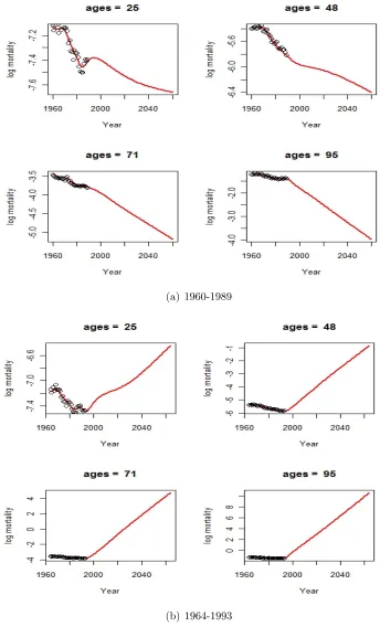
ap-plication sometimes leads to bizarre results. For example, Figure 1.1(a) and 1.1(b) display

the projected log mortality rates at different ages from the P-spline method by minimizing

the Bayesian information criterion (BIC), based on female USA mortality data from year

1960-1989 and 1964-1993, respectively. From the figure, we observe that although the

pro-jections in the former case are all well behaved, in the latter case the log mortality rates

xxxi

(a) 1960-1989

(b) 1964-1993

for all sample ages (unrealistically) increase, and even exceed 0 for ages 71 and 95, which is

obviously undesirable. One way to avoid this problem is to target a fixed value of the degree

of freedom (df) instead of minimizing the BIC.9 _{More specifically, by fixing df at 20, we} observe reasonable shapes from all generations. Similarly as in the CBD-Perks model, we

use a reduced age range from 25 to 95 with K = 2485.

1.2.3 Factor Analysis

With ∆ = tj+1 −tj = 1, Proposition 1 implies that ¯Fl(tj, tj+1) are i.i.d. Gaussian so that we can write

¯

Fl(tj, tj+1) =a+bZj +j, (1.2)

with coefficients a ∈ _RK_{, b ∈}

RK×d, factors Zj ∈ Rd with E(Zj) = 0 and Cov(Zj) = Id×d,

and an error termj ∈RK with E(j) = 0 and Cov(j) = diag(ψ1, . . . , ψK).

Estimates of a, b, and the number of factors, d, can be obtained from a principal

component analysis on the time series of ¯Fl(tj, tj+1), j = 1,2, . . . , N −1. This is akin to the fixed income literature (see e.g. Litterman and Scheinkman (1991) or Rebonato (1998)),

and several authors have taken a similar approach to the analysis of period mortality data

(see e.g. Lee and Carter (1992) or Njenga and Sherris (2009)). However, thus far, there has

been no attempt to analyze generational mortality data in order to identify the drivers of

the entire age/term structure of mortality. The procedure is standard: We first compute the

xxxiii

empirical covariance matrix of ¯Fl(tj, tj+1), ˆΣ, then decompose it as

ˆ

Σ = U ×

           

λ1 0 · · · 0

0 λ2 0

..

. . .. ...

0 0 · · · λK

           

×U0 =

K

X

ν=1

λνuνu0ν,

where U = (u1, u2,· · · , uK) is an (orthogonal) matrix consisting of the eigenvectors of ˆΣ,

and λν, ν = 1,2, . . . , K, are the corresponding eigenvalues in decreasing order. We then

pick thedgreatest eigenvalues that explain the majority of the variation in the data, e.g. we

choose d such that

Pd

ν=1λν

PK

ν=1λν

≥ξ,

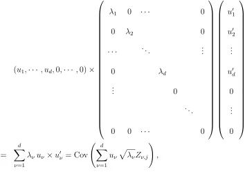
Notice that the resulting approximative covariance matrix is

(u1,· · · , ud,0,· · ·,0)×

                       

λ1 0 · · · 0

0 λ2 0

· · · . .. ...

0 λd

..

. 0

. ..

0 0 · · · 0

                                               

u0₁

u0₂

.. .

u0_d

0 .. . 0                         = d X ν=1

λνuν ×u0ν = Cov d

X

ν=1 uν

p

λνZν,j

!

,

whereZν,jare i.i.d. (scalar) standard Normal random variables,ν, j ∈ {1, . . . , d}×{1, . . . , N−

1}. Hence, isolating the firstd eigenvalues suggests the representation

¯

Fl(tj, tj+1) =E

_¯

Fl(tj, tj+1)

+ d X ν=1 uν p

λνZν,j+j, (1.3)

i.e. a = _EF¯l(tj, tj+1)

and b = u1

√

λ1, . . . , ud

√ λd

in Equation (1.2). In what follows,

we conduct the factor analysis on each data set with generations from all three forecasting

methodologies, respectively.

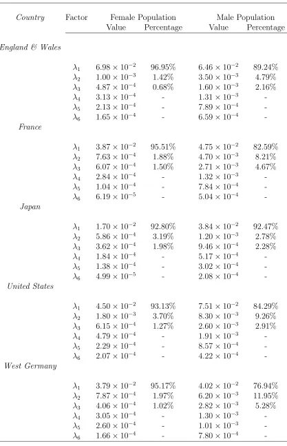
The Lee-Carter Approach Table 1.1 shows the six greatest eigenvalues (λν, ν =

1, . . . ,6) for different populations under the Lee-Carter approach. From the table, we observe

xxxv

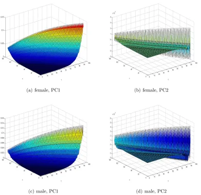
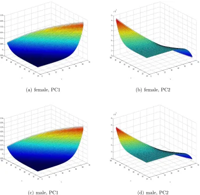
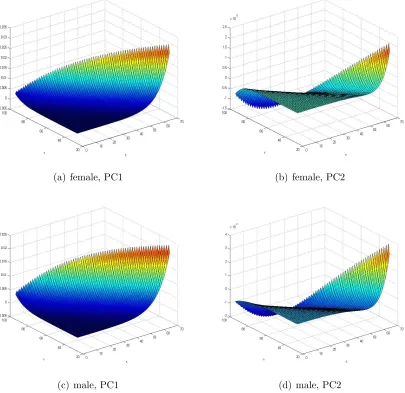
(a) female, PC1 (b) female, PC2

(c) male, PC1 (d) male, PC2

Figure 1.2. Eigenvectors for the ENW data, Lee-Carter model

total variation. Moreover, by comparing data sets between genders, we find that higher

(ab-solute) variances emerge from the male population, whereas the first eigenvalue has greater

explanatory power (higher weight) for the female population in all sample sets.

The eigenvectors associated the two largest eigenvalues as functions of τ and x for

Country Factor Female Population Male Population Value Percentage Value Percentage

England & Wales

λ1 6.98×10−2 96.95% 6.46×10−2 89.24% λ2 1.00×10−3 1.42% 3.50×10−3 4.79% λ3 4.87×10−4 0.68% 1.60×10−3 2.16%

λ4 3.13×10−4 - 1.31×10−3

-λ5 2.13×10−4 - 7.89×10−4

-λ6 1.65×10−4 - 6.59×10−4

-France

λ1 3.87×10−2 95.51% 4.75×10−2 82.59% λ2 7.63×10−4 1.88% 4.70×10−3 8.21% λ3 6.07×10−4 1.50% 2.71×10−3 4.67%

λ4 2.84×10−4 - 1.32×10−3

-λ5 1.04×10−4 - 7.84×10−4

-λ6 6.19×10−5 - 5.04×10−4

-Japan

λ1 1.70×10−2 92.80% 3.84×10−2 92.47% λ2 5.86×10−4 3.19% 1.20×10−3 2.78% λ3 3.62×10−4 1.98% 9.46×10−4 2.28%

λ4 1.84×10−4 - 5.17×10−4

-λ5 1.38×10−4 - 3.02×10−4

-λ6 4.99×10−5 - 2.08×10−4

-United States

λ1 4.50×10−2 93.13% 7.51×10−2 84.29% λ2 1.80×10−3 3.70% 8.30×10−3 9.26% λ3 6.15×10−4 1.27% 2.60×10−3 2.91%

λ4 4.79×10−4 - 1.91×10−3

-λ5 2.29×10−4 - 8.57×10−4

-λ6 2.07×10−4 - 4.22×10−4

-West Germany

λ1 3.79×10−2 95.17% 4.02×10−2 76.94% λ2 7.87×10−4 1.97% 6.20×10−3 11.95% λ3 4.06×10−4 1.02% 2.82×10−3 5.28%

λ4 3.05×10−4 - 1.30×10−3

-λ5 2.60×10−4 - 1.01×10−3

-λ6 1.66×10−4 - 7.80×10−4

xxxvii

exhibited and are thus omitted to keep the presentation concise).10 _{We observe that the}

structure of the first principal component is primarily governed by an increasing age/term

effect, which may be the key reason for its dominant role in explaining the variation of the

generational mortality data. Moreover, we find that the forward forces of mortality for high

ages in the far future appear to be more volatile than those in the near future, a feature

that is not captured by most mortality forecasting approaches—particularly mean-reverting

ones. Therefore, we refer to the first factor as the slope factor.

As for the second principal component, for some data sets (e.g. female ENW) it looks

rather unsystematic, whereas for others (e.g. male JPN) we observe a consistently over time

decreasing influence that even generates an inverse relationship for higher ages in the near

and the far future (generally this factor is more clearly observed from male population data

sets). It is therefore referred to as thetwist factor.

Considering both the weights of eigenvalues and shapes of eigenvectors, in what follows

we choose the number of drivers,d, to be 1 for female populations, and 2 for male populations

in the Lee-Carter case.

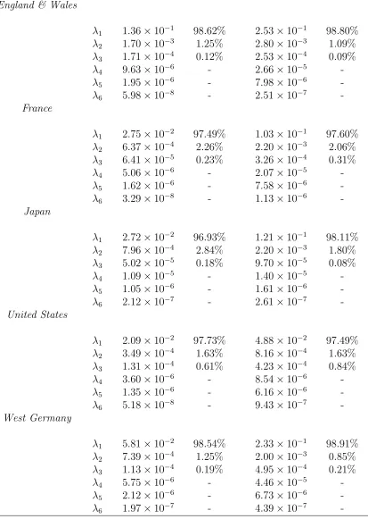
The CBD-Perks Model Table 1.2 shows the six greatest eigenvalues for different populations under the CBD-Perks model. From the table, we observe that the first eigenvalue

takes an even more dominant role in all data sets compared with the Lee-Carter approach,

and that there is no considerable difference between male and female populations in the

(a) female, PC1 (b) female, PC2

(c) male, PC1 (d) male, PC2

Figure 1.3. Eigenvectors for the ENW data, CBD-Perks Model

planation power of the first eigenvector. However, we still observe that the male populations

still possess higher absolute variations across all selected countries/regions.

The eigenvectors associated with the two largest eigenvalues as functions ofτ and xfor

England & Wales are displayed in Figure 1.3. We find that the first principal component

exhibits essentially the same shape as in the Lee-Carter case across all data sets, which implies

xxxix

Country Factor Female Population Male Population Value Percentage Value Percentage

England & Wales

λ1 1.36×10−1 98.62% 2.53×10−1 98.80% λ2 1.70×10−3 1.25% 2.80×10−3 1.09% λ3 1.71×10−4 0.12% 2.53×10−4 0.09%

λ4 9.63×10−6 - 2.66×10−5

-λ5 1.95×10−6 - 7.98×10−6

-λ6 5.98×10−8 - 2.51×10−7

-France

λ1 2.75×10−2 97.49% 1.03×10−1 97.60% λ2 6.37×10−4 2.26% 2.20×10−3 2.06% λ3 6.41×10−5 0.23% 3.26×10−4 0.31%

λ4 5.06×10−6 - 2.07×10−5

-λ5 1.62×10−6 - 7.58×10−6

-λ6 3.29×10−8 - 1.13×10−6

-Japan

λ1 2.72×10−2 96.93% 1.21×10−1 98.11% λ2 7.96×10−4 2.84% 2.20×10−3 1.80% λ3 5.02×10−5 0.18% 9.70×10−5 0.08%

λ4 1.09×10−5 - 1.40×10−5

-λ5 1.05×10−6 - 1.61×10−6

-λ6 2.12×10−7 - 2.61×10−7

-United States

λ1 2.09×10−2 97.73% 4.88×10−2 97.49% λ2 3.49×10−4 1.63% 8.16×10−4 1.63% λ3 1.31×10−4 0.61% 4.23×10−4 0.84%

λ4 3.60×10−6 - 8.54×10−6

-λ5 1.35×10−6 - 6.16×10−6

-λ6 5.18×10−8 - 9.43×10−7

-West Germany

λ1 5.81×10−2 98.54% 2.33×10−1 98.91% λ2 7.39×10−4 1.25% 2.00×10−3 0.85% λ3 1.13×10−4 0.19% 4.95×10−4 0.21%

λ4 5.75×10−6 - 4.46×10−5

-λ5 2.12×10−6 - 6.73×10−6

-λ6 1.97×10−7 - 4.39×10−7

methodology. For the second principal component, similarly, a twisted shape is observed

across all data sets. However, the explanation power for the twist factor is relatively small.

Considering both the weights of eigenvalues and shapes of eigenvectors, we assumedto

be 1 for both female and male populations in the CBD-Perks case.

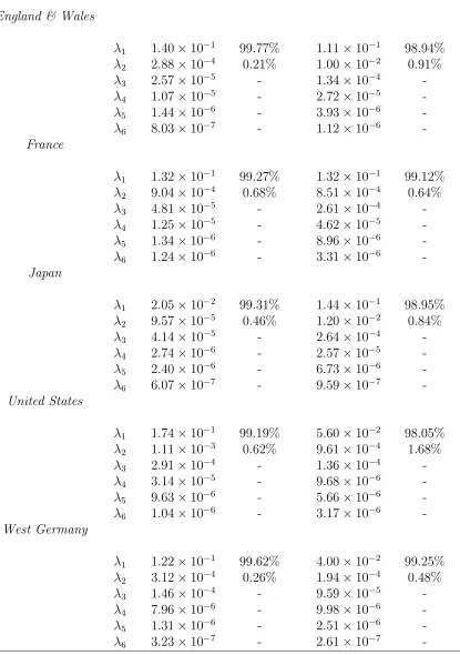
The P-spline Method Table 1.3 shows the six greatest eigenvalues for different populations under the P-spline method. From the table, we observe that similarly to the

CBD-Perks case, the first eigenvalue takes a highly dominant role in all cases, and that there

is no considerable difference between male and female population in the explanation power

of the first principal component.

Again, the eigenvectors for the two largest eigenvalues as functions of τ and x for

England & Wales are displayed in Figure 1.4, and we observe that again both the first and

the second principal components exhibit similar shapes (“slope” and “twist”). Since the

first eigenvalue takes an extremely dominant role, we choosed= 1 for both female and male

populations in the P-spline case.

1.2.4 Simple Factor Models

From the factor analysis, we can devise simple factor models that can be used as simple,

easy-to-estimate mortality forecasting methodologies. Specifically, notice that Equation (1.3)

is essentially a regression equation with unknownZν,j. By assuming that the firstdprinciple

components are portrayed by the model without error (see e.g. Diebold and Li (2006) or Joslin

xli

Country Factor Female Population Male Population Value Percentage Value Percentage

England & Wales

λ1 1.40×10−1 99.77% 1.11×10−1 98.94% λ2 2.88×10−4 0.21% 1.00×10−2 0.91%

λ3 2.57×10−5 - 1.34×10−4

-λ4 1.07×10−5 - 2.72×10−5

-λ5 1.44×10−6 - 3.93×10−6

-λ6 8.03×10−7 - 1.12×10−6

-France

λ1 1.32×10−1 99.27% 1.32×10−1 99.12% λ2 9.04×10−4 0.68% 8.51×10−4 0.64%

λ3 4.81×10−5 - 2.61×10−4

-λ4 1.25×10−5 - 4.62×10−5

-λ5 1.34×10−6 - 8.96×10−6

-λ6 1.24×10−6 - 3.31×10−6

-Japan

λ1 2.05×10−2 99.31% 1.44×10−1 98.95% λ2 9.57×10−5 0.46% 1.20×10−2 0.84%

λ3 4.14×10−5 - 2.64×10−4

-λ4 2.74×10−6 - 2.57×10−5

-λ5 2.40×10−6 - 6.73×10−6

-λ6 6.07×10−7 - 9.59×10−7

-United States

λ1 1.74×10−1 99.19% 5.60×10−2 98.05% λ2 1.11×10−3 0.62% 9.61×10−4 1.68%

λ3 2.91×10−4 - 1.36×10−4

-λ4 3.14×10−5 - 9.68×10−6

-λ5 9.63×10−6 - 5.66×10−6

-λ6 1.04×10−6 - 3.17×10−6

-West Germany

λ1 1.22×10−1 99.62% 4.00×10−2 99.25% λ2 3.12×10−4 0.26% 1.94×10−4 0.48%

λ3 1.46×10−4 - 9.59×10−5

-λ4 7.96×10−6 - 9.98×10−6

-λ5 1.31×10−6 - 2.51×10−6

-λ6 3.23×10−7 - 2.61×10−7

(a) female, PC1 (b) female, PC2

(c) male, PC1 (d) male, PC2

xliii

ν = 1, . . . , d, are orthogonal to each other, we have

Yν(j) 4

= (uν

p

λν)TF¯l(tj, tj+1)

= (uν

p

λν)TE[ ¯Fl] +λνZν,j, ν = 1, . . . , d. (1.4)

Therefore, Equation (1.3) can be modified as

¯

Fl(tj, tj+1) = E

_¯

Fl(tj, tj+1)

+ d X ν=1 uν √ λν

[Yν(j)−(uν

p

λν)TE[ ¯Fl(tj, tj+1)]] +j

4

= m˜ +

d

X

ν=1 ˜

sν×Yν(j) +j, (1.5)

which is a regression equation of ¯Fl(tj, tj+1) on the knownYν(j), and the constant and linear

coefficients ˜m, ˜sν, ν = 1, . . . , d can be easily obtained from OLS regression.

The above factor model can then be used to generate forecasts of mortality projections:

From the i.i.d. normality of Zν,j we know that Yν(j) are also i.i.d. Normal distributed, and

we denote the directly calculated sample mean and standard error of Yν(j) as (µsY,ν, σY,νs ).

Therefore, we can simulate Yν(N)∼N(µsY,ν, σY,νs ). A forecast is then given by

¯

Fl(tN, tN+1) = ˜m+

d

X

ν=1 ˜

sν ×Yν(N),

from which together with known τpx(tN), we can derive τpx(tN+1), i.e. we can simulate the

Methodology Test i.i.d. Normality

Lee-Carter √ √

CBD-Perks √ √

P-spline × √

Table 1.4. Tests for i.i.d. and Normality

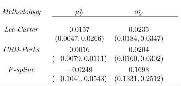
Methodology µs

Y σsY

Lee-Carter 0.0157 0.0235

(0.0047,0.0266) (0.0184,0.0347)

CBD-Perks 0.0016 0.0204

(−0.0079,0.0111) (0.0160,0.0302)

P-spline −0.0249 0.1698 (−0.1041,0.0543) (0.1331,0.2512)

Table 1.5. Sample Means and Standard Variances

We use the female USA data for an illustration, where we choose d = 1 as indicated

above. First, we test if the sample data is actually i.i.d. (Ljung-Box test) and Normal

distributed (Jarque-Bera test), where we use a confidence level of 95%. The test results are

displayed in Table 1.4 for all three underlying mortality projection methodologies. From the

table, we see that the i.i.d. assumption is rejected for the data set that are generated under

theP-spline method, which suggests possible serial correlation in{Y(j)}. We then calculate

{Y(j)} under each projection methodology, and regress ˜m and ˜sν. The associated (µsY, σ s Y)

xlv

1.3 Forward Mortality Factor Models

1.3.1 Theory

While the simple factor models proposed in the previous section present simply,

easy-to-estimate approaches to forecasting mortality projections, they do not account for the

inherent structure that arises from the interpretation of the data as forecasts. More precisely,

for the forecasts to be self-consistent, the expected value of forecasts should align with the projection engrained in the cross-section of the data. For instance, the expected value of next

year’s realized survival rates should coincide with the projection in this year’s generational

mortality table.

So-called forward mortality models adhere to this relationship. In what follows, we

briefly outline the relevant theory borrowing from Bauer et al. (2012). Subsequently, we

demonstrate how these results—in conjunction with the results from the previous section—

can be employed to develop simple parametric models for mortality forecasts.

Mathematically, self-consistency of a dynamic model for mortality forecasts takes the form of a martingale property. More specifically, expected realized mortality rates should

align with the given forecasts:11

Et

exp

−

Z T

0

µs(0, x0+s)ds

= exp

−

Z t

0

µs(0, x0 +s)ds

T−tpx0+t(t), (1.6)

i.e.expn−Rt

0 µs(0, x0+s)ds

o

T−tpx0+t(t)

t≥0

are martingales. This yields a self-consistency

condition akin to the well-known HJM (drift) condition for forward-interest rate models (cf.

11_{As usual in this context,}

Cor. 3.1 in Bauer et al. (2012)) which links the drift component and the volatility component

of µt(τ, x):

α(τ, x) = σ(τ, x)×

Z τ

0

σ0(s, x)ds. (1.7)

As before, we are interested in factor models

µt(τ, x) = G(τ, x;Zt),

where G is a known deterministic function and Zt is some convenient finite-dimensional

random variable (so that (Zt)t≥0 is some convenient stochastic process). Proposition 4.1 in Bauer et al. (2012) shows that for the time-homogeneous Gaussian models considered here,

the volatility structure must necessarily be of the form

σ(τ, x) =C(x+τ)×exp{M τ} ×N, (1.8)

where N ∈_Rm×d_{, M ∈}

Rm×m, and C0 ∈C1([0,∞),Rm) ; the factor model is then given by

µt(τ, x) =µ0(τ+t, x−t)+ Z t

0

α(τ+t−s, x−t+s)ds+C(x+τ) exp{M τ} Z t

0

exp{M(t−s)}N dWs

| {z }

=Zt

.

(1.9)

For a given number of drivers (d) from the factor analysis, the above semi-parametric

xlvii

1.3.2 Econometrical Approach

We starting by noting the following proposition which will prove to be convenient in

what follows.12

Proposition 2

Letσ(τ, x) = (σ1(τ, x), . . . , σd(τ, x)), where each function σi(τ, x)is of the form

σi(τ, x) =Ci(x+τ)×exp{Miτ} ×Ni, (1.10)

Ci(·) ∈ R1×mi, Mi ∈ Rmi×mi, Ni = Rmi×1, mi ∈ N, i = {1,2, . . . , d}. Then σ(τ, x) is also

of the form (2.3), i.e. the model implied by σ(τ, x) allows for a Gaussian realization, where

C(x) = [C1(x), . . . , Cd(x)], M =diag{M1, . . . , Md}, and N =diag{N1, . . . , Nd}.

A proof is provided in Section 1.7. Proposition 2 essentially allows us to treat each

independent factor separately.

With some basic manipulations, we obtain

Fl(tj, tj+1,(τ, x))

d

=

Z tj+1−tj 0

Z τ+l

τ

α(v+tj+1−tj −s, x−tj+1+tj+s)dv ds

+

Z tj+1−tj 0

Z τ+l

τ

C(x+v) exp{M(v+tj+1−tj −s)} N dv dWs d

=

Z tj+1−tj 0

Z τ+l

τ

α(v+tj+1−tj −s, x−tj+1+tj+s)dv ds

+

Z τ+l

τ

C(x+v) exp{M v} dv

| {z }

=O(τ,x)

×

Z tj+1−tj 0

exp{M(tj+1−tj −s)} N dWs

| {z }

=Z_tj+1−_tj

(1.11)

is Normal distributed.

Furthermore, from Proposition 2 and Equation (1.11), for the model with volatility

structure σ(τ, x) = (σ1(τ, x), . . . , σd(τ, x)) as in (1.10), we obtain in analogy to Equation

(1.3)

¯

Fl(tj, tj+1)

d

≈ _E¯

Fl(tj, tj+1)

+

d

X

ν=1

(ω(τi, xi)×Oν(τi, xi))1≤i≤K

×√ 1 tj+1−tj

Z tj+1−tj 0

exp{Mν(tj+1−tj −s)}NνdWs(ν), (1.12)

where Oν(τi, xi) =

Rτi+l

τi Cν(xi +s) exp{Mνs} ds and 1

√

tj+1−tj

Rtj+1−tj

0 exp{Mν(tj+1 −tj − s)}NνdW

(ν)

s is an mν-dimensional vector of Normal random variables, 1 ≤ ν ≤ d. While

this vector may not necessarily consist of perfectly correlated random variables, they are all

driven by the same (scalar) Brownian motion and will thus be strongly related. In particular,

for a short time step (tj+1−tj), the standard Euler scheme yields an approximation by a

perfectly correlated random vector

1

√

tj+1−tj

Z tj+1−tj 0

exp{Mν(tj+1−tj−s)}NνdWs(ν)

≈ √ 1

tj+1−tj

exp{Mν(tj+1−tj)}Nν(W

(ν)

tj+1−tj−W (ν) 0 )

| {z }

d

=√tj+1−tjZ˜ν,j

= exp{Mν(tj+1−tj)}Nν

| {z }

≡N˜ν,j∈Rmν

×Z˜ν,j, (1.13)

where ˜Zν,j again are standard Normal random variables and independent for different ν, j ∈

xlix

and setting ω(τ, x)≡1 as before, we obtain

(Oν(τi, xi))1≤i≤K×N˜ν ≈uν

p

λν, 1≤ν ≤d. (1.14)

Now Proposition 2 implies that we may examine each component σν(τ, x) and, hence,

each eigenvectoruν, separately,ν ∈ {1, . . . , d}. To simplify notation, we assume (tj+1−tj) =

∆, although similar relationships hold for non-equidistant data. From Equations (1.13) and

(1.14), we obtain for small l (here l=1)

uν

p

λν ≈ (Oν(τi, xi))1≤i≤K×N˜ν,j =

Z τi+l

τi

Cν(xi+s) exp{Mνs}ds

1≤i≤K

×N˜ν,j

≈ (Cν(xi+τi+l/2)×exp{Mν(τi+l/2)} ·l)1≤i≤K×exp{Mν∆} ×Nν

= (Cν(xi+τi+ 1/2)×exp{Mν(τi+ 1/2 + ∆)} ×Nν)1≤i≤K. (1.15)

Based on Equation (1.15), we are now able to estimate Cν(x), Mν, and Nν via regression.

Note, however, that in doing so, we are only utilizing the variance part of ¯Fl(tj, tj+1), with

all information on _EF¯l(tj, tj+1)

being neglected (cf. Equation (2.2)). Furthermore, the

underlying approximations may lead to a slight bias in our estimation of the parameters.

Therefore, we are not going to finalize the estimation of the parameter values here, but

rather rely on the gained insights to determine suitable functional assumptions for Cν(·) as

well as structures for Mν and Nν. The actual estimation of the parameter values based on

Moreover, a direct (unconstrained) regression brings about problems. More specifically,

choosing mi ≡ 1 heavily constrains possible shapes since the matrix exponential is

one-dimensional, whereas mi > 1 leads to identification problems. Thus, here we take a two

step identification procedure: In the first step, we investigate Mν andNν without specifying

any functional assumption on Cν(x) by relying on examples from interest rate modeling

(see, e.g. Bj¨ork and Gombani (1999)) that are able to capture the term shapes displayed by

the eigenvectors (cf. Figures 1.2, 1.3, and 1.4); in the second step, in order to reduce the

number of parameters to make the calibration procedure tractable, we determine appropriate

functional assumptions for Cν(x), which can then be employed in the maximum likelihood

estimation.

The Slope Factor Since the slope factor is observed across all sample populations, we impose the same assumption throughout all cases. We choose m1 = 2 and set

C1(x+τ) = f(x+τ)×

0 1

,

M1 =

   

−2b −b2

1 0

   

,and

N1 =

   

1−ab a

   

li

which is a slight modification of Example 6.2 in Bj¨ork and Gombani (1999), and obtain

σ1(τ, x) = f(x+τ)×

0 1 ×exp    

−2bτ −b2τ

τ 0     ×    

1−ab a

   

= f(x+τ)(a+τ) exp(−bτ).

This functional form is specifically chosen to capture the increasing, concave shape of the

“diagonal curves” observed in the surfaces.

With above specifications, from Equation (1.15) we can approximate

u1

p

λ1 =

Z τ+l

τ

σ1(s+ ∆, x−∆) ds≈σ1

τ + ∆ + l

2, x−∆

·l

= f

x+τ+ l

2 a+τ+ ∆ +

l 2 exp −b

τ+ ∆ + l 2

·l.

Notice that even withm1 = 2,f(x+τ) is one-dimensional, and there only exists one driving

Brownian motion. A non-parametric regression yields the function f(·) (see Figure 1.5). We find that in all cases, a logistic-Gompertz function,

f(x) = k× exp(cx+d)

(1 + exp(cx+d))

is an appropriate choice to fitf(·). To illustrate, in addition to the non-parametric regression function, Figure 1.5 displays the logistic-Gompertz functional fit from the nonlinear

least-squares estimation for USA data (similar figures are obtained for other countries and are

(a) female, Lee-Carter (b) male, Lee-Carter

(c) female, CBD-Perks (d) male, CBD-Perks

(e) female, P-spline (f) male,P-spline

liii

The Twist Factor Since the weight of the second eigenvalue is small relative to the first one, we assume m2 = 1 for the sake of parameter parsimony. That is,

σ2(τ, x) =C2(x+τ)×exp(M2τ)×N2,

M2 ∈R, N2 ∈R, therefore, N2 can be further integrated into C2(x+τ). Similarly as in the analysis of the first factor, we can approximate

u2

p

λ2 =

Z τ+l

τ

σ2(s+ ∆, x−∆) ds ≈σ2

τ+ ∆ + l

2, x−∆

·l

= C2

x+τ+ l 2

exp

M2

τ+ ∆ + l 2

·l.

Furthermore, from a corresponding non-parametric regression (cf. Figure 1.6), we

ob-serve that the decreasing-then-increasing shape ofσ2(τ, x) can be well captured by choosing

C2(·) as the difference between two logistic-Gompertz functions

C2(x) = k1

exp(c1x+d1) 1 + exp(c1x+d1)

−k2

exp(c2x+d2) 1 + exp(c2x+d2)

.

To further reduce the number of parameters, we require c1 =c2, andk1−k2 = 1. The latter requirement is also useful in setting a possible upper bound of the volatility, which is implied

by the natural boundedness of mortality rates. In addition to the non-parametric regression,

(a) ENW (b) USA

Figure 1.6. Fitting C2(x) with Logistic-Gompertz function, male population, Lee-Carter method

1.3.3 Maximum Likelihood Estimation

Similarly as in the factor analysis, we rely on the quantitiesFl(tj, tj+1,(τ, x)), (τ, x)∈C˜ as the basis for our estimation. In particular, we can express Equation (1.11) as:

Fl(tj, tj+1,(τ, x)) = −log

τ+lpx(tj+1, tj+1+τ+l)

τpx(tj+1, tj+1+τ)

τ+l+tj+1−tjpx−tj+1+tj(tj, tj+1+τ +l)

τ+tj+1−tjpx−tj+1+tj(tj, tj+1+τ)

=

Z tj+1

tj

Z l

0

α(v+τ+tj+1−s, x−tj+1+s)dv ds

+

Z tj+1

tj

Z l

0

σ(v +τ +tj+1−s, x−tj+1+s)dv dWs.

Therefore, with Equation (2.2),Fl(tj, tj+1,(τ, x)) is Normal distributed with expected value

E[Fl(tj, tj+1,(τ, x))] =

Z tj+1

tj

Z l

0

σ(v+τ+tj+1−s, x−tj+1−s)

Z v+τ+tj+1−s

0

lv

and covariance structure

Cov [Fl(tj, tj+1,(τ1, x1)), Fl(tk, tk+1,(τ2, x2))] =

δjk× Z tj+1

tj

Z l

0

σ(v+τ1+tj+1−s, x1−tj+1+s)dv

Z l

0

σ0(v+τ2+tj+1−s, x2−tj+1+s)dv ds

by a simple application of It¯o’s product formula, in whichδjkequals 1 ifj =kand 0 otherwise.

In particular, fortj+1−tj = ∆,13the vectors ¯Fl(tj, tj+1) = (ω(τ, x)×FL(tj, tj+1,(τ, x)i))₁≤i≤K

are i.i.d. Normal with expected values

¯

µ =

ω(τ, x)

Z ∆

0

1 2

Z l+τ+∆−s

τ+∆−s

σ(u, x−∆ +s)du

Z l+τ+∆−s

τ+∆−s

σ0(u, x−∆ +s)du

+

Z l+τ+∆−s

τ+∆−s

σ(u, x−∆ +s)du

Z τ+∆−s

0

σ0(u, x−∆ +s)du

ds

(τ,x)∈C˜

and covariance matrix Σ = (Σij)1≤i,j≤K, where

Σij =ω(τi, xi)ω(τj, xj)×

Z ∆ 0

Z l

0

σ(v+τi+∆−s, xi−∆+s)dv

Z l

0

σ0(v+τj+∆−s, xj−∆+s)dv ds.

Similar ideas were applied in Bauer et al. (2008a) and Bauer (2009) for their

maximum-likelihood calibration algorithms. However, as pointed out in their contributions, such an

approach only allows for the consideration of a (very) small number of term/age combinations

(τi, xi) (i.e. a small value ofK) since (non-systematic) deviations are not admissible. In order

to overcome this problem, we allow for non-systematic deviations in the “observed” vectors

13_{Similarly as above, we consider this special case for notational convenience, while analogous results also}

¯

Fobs_(t

j, tj+1) from our model-endogenous vectors ¯Fmod(tj, tj+1). More specifically, we assume

¯

Fobs(tj, tj+1) = ¯Fmod(tj, tj+1) +j, (1.16)

where_j are mutually independent and independent of ¯Fmod_(t

j, tj+1),j ∼N(0, α·diag{Σ}),

j = 1, . . . , N −1, in which α is the sum of the weights of all other eigenvalues that are not considered within our model specification. Intuitively, the _j pick up the variation not

accounted for by the considered first d factors. Thus, we obtain

¯

Fobs(tj, tj+1)∼N(¯µ,Σ)˜ , (1.17)

where ˜Σ = Σ +α·diag{Σ} and the log-likelihood function is of the form

L( ¯Fobs(t1, t2), . . . ,F¯obs(tN−1, tN);C, M, N, σe)

= log    N Y j=2 1 q

(2π)K_{det( ˜Σ)}

exp

−1

2( ¯F

obs_(t

j−1, tj)−µ¯) ˜Σ−1( ¯Fobs(tj−1, tj)−µ¯)0

   = 1 2 " _N X j=2

−logndet( ˜Σ)o−( ¯Fobs(tj−1, tj)−µ¯) ˜Σ−1( ¯Fobs(tj−1, tj)−µ¯)0

#

| {z }

≡_L˜

+const.(1.18)

To determine maximum likelihood estimates for our model parameters, it now suffices to

determine the maximum values for ˜L, which can be carried out numerically for each case.

lvii

Country Parameters L˜

k c d a b

England & Wales 0.0026 0.0718 −9.9728 40.8339 0.0025 −5.2796×104

France 0.0015 0.0711 −10.3398 37.4549 0.0074 7.8626×104

Japan 0.0012 0.0696 −10.1860 41.2554 0.0114 7.4379×104

United States 0.2145 0.0652 −13.6249 14.7317 0.0048 −5.9389×104

West Germany 0.0002 0.0712 −8.1509 20.5784 0.0071 9.0568×104

Table 1.6. The MLE results for female population – Lee-Carter Model

The Lee-Carter Approach Recall that d = 1 for female populations and d= 2 for male populations under the Lee-Carter forecasts. Table 1.6 and 1.7 display the estimated

parameter values together with values of ˜L for female populations and male populations,

respectively.

The CBD-Perks Model For the CBD-Perks model, recall that d = 1 for both female and male populations. The estimated parameter values together with values of ˜L are

displayed in Table 1.8 and 1.9 for female and male populations, respectively.

The P-spline Method For theP-spline method, similarly,d= 1 for both female and male populations. The estimated parameter values together with values of ˜L are displayed