Assessment of shallow subsurface characterisation with non invasive geophysical methods at the intermediate hill slope scale

(1)

Hydrol. Earth Syst. Sci., 17, 1297–1307, 2013 www.hydrol-earth-syst-sci.net/17/1297/2013/ doi:10.5194/hess-17-1297-2013

EGU Journal Logos (RGB)

Advances in

Geosciences

Open Access

Natural Hazards

and Earth System

Sciences

Open Access

Annales

Geophysicae

Open Access

Nonlinear Processes

in Geophysics

Open Access

Atmospheric

Chemistry

and Physics

Open Access

Atmospheric

Chemistry

and Physics

Open Access Discussions

Atmospheric

Measurement

Techniques

Open Access

Atmospheric

Measurement

Techniques

Biogeosciences

Open Access Open Access

Biogeosciences

Discussions

Climate

of the Past

Climate

of the Past

Discussions

Earth System

Dynamics

Earth System

Dynamics

Discussions

Geoscientific

Instrumentation

Methods and

Data Systems

Open Access

_{Geoscientific}

Instrumentation

Methods and

Data Systems

Geoscientific

Model Development

Geoscientific

Model Development

Discussions

Hydrology and

Earth System

Sciences

Open Access

Hydrology and

Earth System

Sciences

Ocean Science

Discussions

Solid Earth

Discussions

The Cryosphere

Discussions

Natural Hazards

and Earth System

Sciences

Open Access

Discussions

Assessment of shallow subsurface characterisation with non-invasive

geophysical methods at the intermediate hill-slope scale

S. Popp, D. Altdorff, and P. Dietrich

UFZ, Helmholtz Centre for Environmental Research, Department Monitoring and Exploration Technologies, Leipzig, Germany

Correspondence to: S. Popp ([email protected]) and P. Dietrich ([email protected])

Received: 26 January 2012 – Published in Hydrol. Earth Syst. Sci. Discuss.: 24 February 2012 Revised: 2 February 2013 – Accepted: 9 March 2013 – Published: 2 April 2013

Abstract. Hill-slopes of several hectares in size represent a difficult scale for subsurface characterisation, as these land-scape units are well beyond the scope of traditional point-scale techniques. By means of electromagnetic induction (EMI) and gamma-ray spectroscopy, spatially distributed soil proxy data were collected from a heterogeneous hill-slope site. Results of EMI mapping using the EM38DD showed that soil electrical conductivity (ECa) is highly variable at both temporal and spatial scales. Calibration of the integral ECa signal to a specific target like soil moisture is hampered by the ambiguous response of EMI to the clay-rich hill-slope underground. Gamma-ray results were obtained during a sin-gle survey, along with EMI measurements and selected soil sampling. In contrast to ECa, a noticeable correlation be-tween Total Count and K emission data and soil-water con-tent seemed to be present. Relevant proxy variables from both methods were used fork means clustering in order to distinguish between hill-slope areas with different soil con-ditions. As a result, we obtained a suitable partition of hill-slope that was comparable with a previously obtained zona-tion model based on ecological factors.

1 Introduction

Exploration of near-surface ground on hill-slopes still poses a significant challenge in hydrological or natural-hazard sci-ences due to subsurface heterogeneity at intermediate land-scape scales (commonly less than one square kilometre). Point measurements, e.g., in situ soil-moisture determina-tion by specific probes or sediment sampling for laboratory analyses provide quantitative data, however, only from a very

limited area or volume of the subsurface. As point measures are relatively costly and time consuming, sampling is often limited to a few selected points. Scaling up point data in order to infer information for the entire hill-slope area is problem-atic, with respect to the heterogeneous underground.

(2)

prediction, the relationship between ECa and the target quan-tity has to be analysed, which is commonly realised by point measures. EMI-based soil-moisture determination, for ex-ample, was successfully achieved at flat, relatively homoge-neous and rather small sites with a significant effort for nu-merous point measures (see cited studies).

Generally, one has to face uncertainties due to different sample volumes of EMI method with regard to the target in the subsurface, which is commonly a soil sample from a specific depth. These uncertainties become more pronounced with increasing heterogeneity and complexity of the study site. Callegary et al. (2012), therefore, suggest a detailed analysis of depth sensitivity of EMI in order to avoid overes-timations of ECa values at a certain point of measurement that is caused by spatially variable sensitivities within the sample volume of the EMI sensor. While this study pro-vides theoretical consideration of the problem based on nu-merical simulations, experimental results from hill slopes show the difficulties of EMI application in an environment, where spatial heterogeneity exceeds those of the senor’s sam-ple volume. For examsam-ple, Tromp-van Meerveld and McDon-nell (2009) gave a nice example of the effort and remain-ing uncertainties for predictremain-ing soil water contents at a rather small hill slope of less than 0.001 km2. The authors achieved a reliable correlation for predicting soil moisture with ECa values, however, only by using individual relationships de-termined at each of the sixty-four measuring points. The use of one (master) relationship for the calculation of water con-tents resulted in a smoothed soil-moisture pattern that did not represent the observed soil-moisture pattern very well. At larger hill-slope scales, Robinson et al. (2012) used a qualita-tive time-lapse approach for revealing relaqualita-tive changes in soil moisture that avoided the problem of calibrating ECa values to individual soil-moisture samples. On the other hand, if the subsurface target is relatively large compared to the sample volume, e.g., soil depth (depth to bedrock), EMI provided suitable results in soil-quality investigations at a large agri-cultural site of nearly 0.2 km2(Zhu et al., 2010a). Generally, the effort required for ground truthing and reliable calibration of EMI results to a relatively small target (soil samples) in-creases significantly in proportion to the size and complexity of the study site for both theoretical and experimental con-siderations. Thus, if adequate soil sampling is not possible or not suitable due to the site conditions or time and cost constraints, other approaches for extracting subsurface infor-mation should be adopted.

In the present study, we have focused on the primary char-acterisation of a large and very heterogeneous hill slope by statistical analysis of geophysical results. For investigation of the hill-slope area, we included a second geophysical method for investigation because of specific site conditions. Under the proposition of a rapid and non-invasive technique we had chosen gamma spectroscopy, because the electrically con-ductive clay-rich subsurface hampered the use of e.g., ground penetrating radar (GPR). Gamma-ray spectroscopy measures

gamma-ray radiation emitted from the natural decay of ra-dioactive elements that are present in rocks and soils (e.g., Minty, 1997; Dickson and Scott, 1997; Wilford et al., 1997). Both the concentration and the ratio of specific radioactive elements can give information on soil properties such as sur-face texture (e.g., Taylor et al., 2002), clay content (e.g., Pracilio et al., 2006), or soil-moisture patterns (e.g., Carroll, 1981; Grasty, 1997).

The goal of this study is the reasonable exploration and characterisation of the hill-slope subsurface based on map-ping of soil proxy values with geophysics. Thereby, we try to minimise the need for invasive measures because soil sam-pling and soil testing are commonly critical points due to time and cost constraints. The number of soil samples is, therefore, restricted to a manageable quantity of less than 20 samples, which are used for a basic evaluation of both methods under site-specific condition. Following the statis-tical approach, we target at a spatially meaningful partition-ing of the heterogeneous subsurface as basis for further de-tailed investigations, and compare the geophysical-based re-sults with a previously obtained hill-slope zonation from hy-drological and soil-survey studies.

2 Material and methods

2.1 Study site

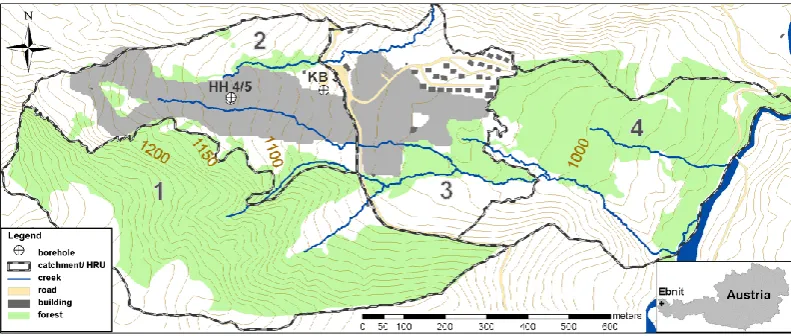
The study area Heumöser (Fig. 1) is located near the Rhine River valley in the western Vorarlberg Alps, Austria, around 10 km south of city of Dornbirn and 0.5 km south of the vil-lage of Ebnit (47◦₂₁0_0.000_{N, 9}◦₄₄0_46.600_{E). The Heumöser} belongs to the head of a steep mountainous catchment and covers 0.95 km2with an extension of 1800 and 500 m in east-west and north-south directions, respectively. The bedrocks that underlie and surround the Heumöser slope are sedimen-tary marlstones from the Upper Cretaceous, belonging to the Alpine Helvetic zone (Lindenmaier et al., 2005). Unweath-ered marlstones are a mixture of calcite, quartz and clay min-erals. The cover sediments, which reach a thickness of up to 40 m, are described as loamy scree and glacial till with vari-able proportions of calcite (up to 40 %), quartz (25–40 %), and clay (up to 30 %) (Schneider, 1999). The water content of these sediments ranges from 20 to 30 %. In soil profiles, water content and proportions of clay can vary and, in partic-ular, the water content can be significantly increased.

(3)

[image:3.595.99.495.62.230.2]

Fig. 1. Topography of the Heum¨oser catchment near Ebnit (Vorarlberg, Austria). The grey-shaded region indicate the open meadow area, on which geophysical mapping was focused. Numbers 1 to 4 denote the major hydrologic units (HRU). HH 4/5 and KB3 indicate the location of boreholes used for inclinometer measurements that specify the surface movement of the slope (see text).

7.5 and 8.5 m depths in KB3 (Schneider, 1999), and between 10.5 and 12.0 m depths in HH4 (Wienh¨ofer et al., 2011).

The geophysical surveys for shallow subsurface explo-ration focus on the accessible meadow areas in the middle and north-western parts of the Heumöser (Fig. 1) between 1039 and 1233 m altitude. This area covers approximately 13 ha with maximum extension of 1030 and 300 m in east-west and north-south directions, respectively. The topogra-phy is highly variable, with relatively steep and hummocky terrain in the west with an average slope angle of 19.5◦, and a rather plane surface in the east. The Heumöser is subdi-vided into four so-called hydrotopes or hydrologic response units (HRU), according to long-term average soil moisture patterns found in detailed botanic and hydropedologic map-ping (Lindenmaier et al., 2005; Wienhöfer et al., 2011). The investigated slope area belongs to HRU 2 and 3, which are generally characterised by very moist to very wet topsoil con-ditions in plane areas, and dryer concon-ditions in bulging areas (Fig. 1). In combination with the significant proportion of clay, the soil surface is electrically high conductive, which hinders the application of GPR and time domain reflectom-etry (TDR). Outcrops of bedrocks additionally prevent inva-sive measures in some places of the hill slope.

2.2 Electromagnetic measurements

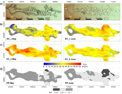
We conducted two electromagnetic mapping surveys at the beginning of May and in the middle of June 2011. The first field survey aimed at a general and rapid characterisation of hill-slope subsurface by “on-the-go” ECa measurements, with an average line spacing of 15 m (Fig. 2a). In June 2011, ECa proximal sensing was conducted as point measurements in conjunction with gamma-ray spectroscopy at 327 loca-tions. Additional soil samples were taken at 18 localoca-tions. The May survey was performed under highly water-saturated soil

conditions, shortly after all snow had fully melted. The sec-ond field measurement in June was assumed to be carried out under changed subsurface conditions (in terms of less water saturated). In all surveys, spatial reference of sampling points was determined by an external D-GPS system (Leica 1200) connected to the EMI recording unit.

We used the EM38DD electromagnetic induction sensor (Geonics Ltd., ON, Canada) for mapping soil electrical con-ductivity. The sensor operates in the frequency domain at fixed coil spacing of 1 m. An alternating current at a spe-cific frequency in the transmitter coil induces a primary electromagnetic field that propagates through the subsurface and generates a secondary magnetic field. The receiver coil detects the primary and secondary magnetic fields at the surface. The ratio of these two readings gives the depth-weighted apparent electrical conductivity (ECa in mS m−1). The EM38DD consist of two EM38 units fixed perpendic-ularly to each other with operating frequencies of 14.6 and 17.0 kHz, respectively. This construction results in two si-multaneous conductivity readings with different depth sponse profiles. The sensor in vertical orientation (EC v) re-ceives its major influence from the shallow subsoil with a common exploration depth of up to 1.5 m (McNeil, 1980b). The horizontally orientated sensor (EC h) is most sensitive to the uppermost topsoil and reaches depths of 0.75 m. Be-fore surveying, the EM38DD sensor was calibrated at the same point on the site according to the user manual at the beginning of each field site measurement day. Additionally, we recorded a reference profile repeatedly both before and in between the measurements in order to check data quality and serviceability of the instrument.

(4)

[image:4.595.99.500.60.370.2]

Fig. 2. EMI measurements from May (left column) and June (right column) with different survey designs and location of reading points (a). White dots in the map on the right show soil sampling locations. The detail views show maps obtained by block ordinary kriging of ECa (mS m−1) using (b) the vertical (EC v) and (c) the horizontal dipole orientation (EC h), as well as (d) the profile ratio (PR). Coordinates on x- and y-axis are in metric BMN M28 Austrian coordinate system.

were removed, while data analysis was performed by ap-plying a filter that only allows for data within the triple of the root-mean-square deviation to be considered. Since soil electrical conductivity can vary due to changes in soil tem-perature, we standardised the field apparent conductivity val-ues to an equivalent conductivity at a reference temperature (25◦_{C) using soil temperatures measured at two locations} on the slope and a conversion function given by Sheets and Hendrickx (1995) and Reedy and Scanlon (2003):

EC25 =ECa

0.4779+1.3801e

−T

25.654

(1) where EC25 is the temperature corrected apparent conduc-tivity, ECais the measured apparent conductivity (mS m−1), andT is the soil temperature (◦C). Soil temperature mea-sured at 10-cm soil depth was in average 8.5 and 15◦C in May and June, respectively. When discussing apparent con-ductivity in the following sections, we always refer to the temperature corrected values. Maps of shallow subsurface apparent conductivity were obtained by variogram analysis and ordinary kriging interpolation, using a 20 m grid.

2.3 Gamma ray spectroscopy

For proximal gamma-ray sensing, we used the portable Ex-ploranium GR256 gamma-ray spectrometer with a 0.35 L thallium activated NaI crystal detector (Exploranium, On-tario, Canada). The gamma sensor detects the gamma radi-ation of variable energies that is emitted by the natural decay of radioactive elements present in rocks and soils. Thereby, about 90 % of the gamma radiation measured at the surface emanates from the upper 30 cm, and about 50 % comes from the top 10 cm (e.g., Cook et al., 1996).

(5)

[image:5.595.139.458.97.185.2]

Table 1. Descriptive statistics of EMI measurements (in mS m−1) in horizontal (EC h) and vertical (EC v) dipole configuration and gamma-ray spectroscopy (in counts per 60 s). SD: standard deviation, CV: coefficient of variation [(SD/Mean)×100].

EC h EC v EC h EC v Gamma Gamma Gamma Total

May May June June K U Th count

Mean 37.1 26.7 31.3 30.4 226 60 36 1230

Min 17.0 1.0 11.8 10.4 44 13 11 393

Max 57.3 52.2 56.5 60.1 583 125 83 2537

SD 6.4 8.0 7.0 8.2 85 17 12 346

CV[%] 17.3 30.0 22.4 27.0 37.6 28.3 33.3 28.1

for kriging interpolation on a 20 m grid analogue to the ECa values.

3 Results and discussion

3.1 Apparent electromagnetic conductivity measurements

Soil electrical conductivity is highly variable on the hill-slope. The overall range of ECa is between 1 and 60 mS m−1, with coefficients of variation (CV) in the range of 17 to 30 % for individual EC h and EC v measurements (Table 1). Dif-ferences data ranges and CV between EC h and EC v dur-ing one survey originate from different sample volumes or exploration depths of the respective dipole orientations. Re-sults of kriging interpolation reveal defined spatial pattern of ECa (Fig. 2b and c) that can be explained in a site-specific context.

In May, soil apparent conductivity shows a significant vertical gradient from a very conductive top soil (EC h sponse) towards less conductive deeper layers (EC v re-sponse) in most parts of the hill-slope. While zones of low EC v readings (<20 mS m−1) in the steeper eastern hill-slope area can be partly attributed to near-surface bed rock (<1 m deep), the high EC h readings are very likely linked to clay-rich soils and/ or high water contents of the top soil after snowmelt. In June, vertical graduation of ECa was less pro-nounced due to decreased conductivity of the top soil. Both the EC h and EC v readings can be used for the calculation of a profile ratio (PR), as an indication for the heterogeneity of the soil column, defined as: PR = EC h/EC v (Corwin et al., 2003; Cockx et al., 2007). A PR close to 1 points to a uniform profile of soil electrical conditions. A PR<1 indi-cates a more conductive subsoil relative to the topsoil, and a PR>1 indicates a conductive topsoil and decreasing conduc-tivity with depth. Figure 2d shows the areas of the hill-slope with different vertical graduations. In May, the majority of the hill-slope subsurface is dominated by conductive top-soil conditions (PR1). The situation had changed in June, where relatively uniform soil conditions (PR∼1) with inter-mediate electrical conductivities prevailed over nearly half of the hill-slope area.

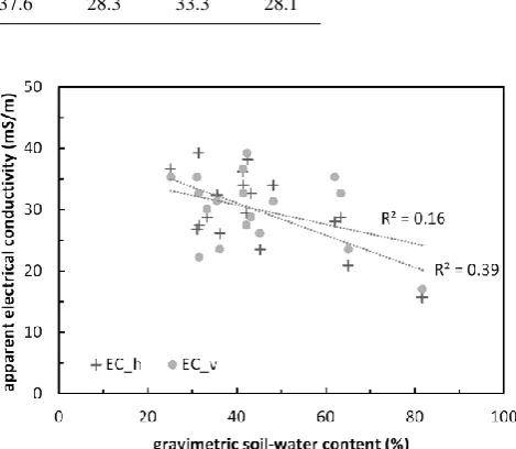
Fig. 3. Scatterplot of gravimetric soil-water content and ECa data, separated into EC h and EC v according to the respective sensor orientation in June survey.

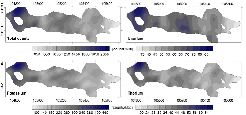
[image:5.595.310.545.174.378.2]

(6)

[image:6.595.98.501.60.248.2]

Fig. 4. Maps of interpolated gamma radiation (in counts per 60 s) using individual data of Total Count (top left panel), potassium or K (bottom left panel) uranium or U (top right panel), and thorium or Th (bottom right panel). Note the different scales of data ranges. Coordinates on x- and y-axis are in metric BMN M28 Austrian coordinate system.

material, which were also evident in the recovered soil sam-ples, are supposed to contribute significantly to the integral signal of soil electrical conductivity. This issue can obviously result in relatively low ECa readings for organic soils even though the soil-water content is high, and vice versa, in rela-tively high ECa values for clayey soils with lower gravimet-ric soil-water content. The distinction between temporally variable soil moisture and the geological background based on a single EMI mapping survey is not possible at the site.

However, given that the type and amount of clay miner-als, soil structure, and ionization of the soil moisture do not change over the considered period of time, ECa variations in repeated measurements are presumably linked to relative changes in soil moisture (Robinson et al., 2009, 2012; Zhu et al., 2010b). On the site, temporal ECa variability is more pronounced in the EC h (topsoil) than in the EC v (subsoil) response. In May, higher apparent conductivities of EC h over wide areas in the steeper west could point to relative higher soil-moisture contents compared to the topsoil condi-tions in June. On the other hand, EC v results show similar spatial pattern in both May and June surveys with low ap-parent conductivity in the steeper west and higher apap-parent conductivities in the eastern part, which could be explained by the stagnic properties of the silty and clayey subsoil. This interpretation is reinforced by findings from a local TDR pro-file measured at the hill-slope, where almost no soil-moisture variation occurred in the deeper subsoil (80 cm depth), while data at a 20 cm depth shows around 10 % of seasonal varia-tion in soil moisture (Lindenmaier et al., 2005).

3.2 Gamma-ray survey

Gamma-ray emission is relatively low at the hill-slope with maximum values of 583, 83 and 125 counts per 60 s for K,

Th and U (Table 1). Total Count, which is the sum signal of all radioactive emissions, reaches maximum 2537 counts per 60 s. Despite the low emission rates and relatively minor data ranges, the variability of gamma-ray flux data is high and more pronounced at smaller spatial scales compared to EMI. For example, gamma-ray flux between two neighbour-ing samplneighbour-ing points can differ significantly from each other due to the small support volume of the gamma-ray method and changing subsurface microstructures. As a result, coeffi-cients of variation are in the range of 28 and 38 % (Table 1). However, regardless of the pronounced small-scale variabil-ity, gamma-ray emission data show definite spatial pattern at the hill-slope scale similar to those of ECa.

(7)

[image:7.595.50.288.62.235.2]

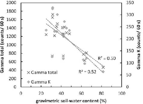
Fig. 5. Scatterplot of gravimetric soil-water content and total gamma counts (left axis) and radioaktive K (right axis).

At the Heum¨oser, the relatively low radioactive emissions are regarded as consequence the of special soil conditions. Soil textures and soil-water contents are mutually depen-dent from each other, e.g., organic or peaty soils can adsorb much more water than mineral soils. Soil moisture in turn increases the bulk density of soils and, thus, the attenuation of gamma radiation, approximately by 1 % for each incre-ment of 1 % volumetric water content (Cook et al., 1996). Lowest gamma-ray emission was, thus, found in places with high soil-water contents. When cross-plotting all obtained gravimetric water contents and gamma-ray data, a notably negative correlation becomes evident with Total Count and K radioactivity measurements (Fig. 5). The higher the soil-water content, the lower the gamma-ray emission. This at-tenuation effect of gamma-ray fluxes, in particular from K and Th with increasing soil moisture, is known from re-sults achieved by airborne gamma-ray measurements and utilised for quantifying soil-water contents based on repeat-edly measured gamma-ray emission (e.g., Carroll, 1981; Grasty, 1997). Similar attenuation effect could be assumed for results obtained from the Heum¨oser based on the rela-tionship in Fig. 5. However, quantification is not possible by means of the snap shot, and qualitative assessment remains arguable to a certain extent without detailed soil analyses. However, taken field descriptions of collected samples into account, a direct proportionality between gamma-ray flux and soil moisture and related soil texture becomes evident. The four samples with high water contents larger than 60 % are organic-rich soils from the eastern part of the slope. The other samples with varying water contents and similar and higher gamma emissions originate from rather mineral soils randomly distributed over the study site. Even though uncer-tainties remain, spatially obtained gamma data allows for a first assessment of soil conditions with emphasis on relative water contents of the topsoil based on the correlation shown in Fig. 5.

Table 2. Results of the PCA: the Component Loadings shows the variance of each variable explained by three factors. Maximum vari-ances of the selected variables for cluster analysis are explained by different factors (italic). Below the respective percentage of the three factors which explain altogether 92 % of total variance.

Component loadings 1 2 3

EC h May 0.358 0.412 −0.833

EC v May −0.692 0.484 −0.101

EC h June −0.016 0.935 0.153

EC v June −0.588 0.740 0.244

Total Count 0.976 0.162 0.087

Gamma K 0.969 0.148 0.084

Gamma U 0.916 0.214 0.136

Gamma Th 0.955 0.147 0.087

Total variance 57.44 24.26 10.35 explained[%]

3.3 Hill-slope characterisation and partitioning

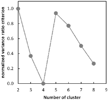
The ambiguous relationship between electrical conductivity and gamma-ray flux and the highly heterogeneous soil prop-erties at the Heum¨oser hamper the straightforward charac-terisation of subsurface structures or soil state variables by means of EMI or gamma-ray spectroscopy. Therefore, we use selected variables from both methods for a joint analy-sis based on a cluster algorithm in order to identify zones of similar soil conditions. The so-called zonal approach (based on e.g.,k means or fuzzyc means clustering) has become a common tool in geophysical data analysis for delineating subsurface structures and estimating petrophysical parame-ters (e.g., Tronicke et al., 2004; Dietrich and Tronicke, 2009; Paasche et al., 2010; Altdorff and Dietrich, 2012). We chose kmeans clustering because of its simple performance and ro-bust results, using the software Systat. Input variables were EC h data from both May and June surveys, as well as To-tal Count gamma-ray data, because these variables provide independent information from a similar shallow exploration depth. Independency was tested by means of principle com-ponent analysis (PCA), in which all variables were included. Results of PCA are shown in Table 2. For thekmeans cluster algorithm, Mahalanobis distance was used as a metric for the measuring distance of data, as it takes the different scales of input variables into account. Cluster analysis was applied on re-gridded data with a 5 m raster that were generated from the kriging interpolation maps shown in Figs. 2 and 4.

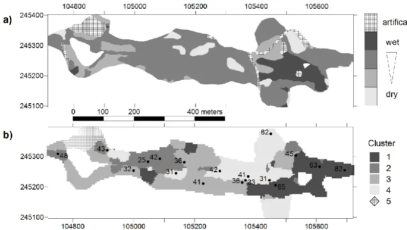
[image:7.595.326.526.127.267.2]

(8)

distance. The optimal solution of this criterion is the number of clusters that maximises the value of the variance criterion. Based on the statistical criterion, a 2 cluster and a 5 clus-ter model would be appropriate results according to the input variables (Fig. 6). Zonation into only two subareas (a steeper northwest, and an eastern part), however, is not a meaningful partitioning of the hill-slope surface with regards to the spa-tially high-resolution geophysical measurements, as well as to further a priori information. We rely on additional infor-mation from an ecological moisture index that has been ob-tained from mapping indicator vegetation and soil cores from the entire catchment (Lindenmaier et al., 2005). This avail-able ecological moisture map discriminates between five dif-ferent classes of soil conditions, thus, the 5 cluster solution appears to be an adequate zonation model for the hill-slope area. A detailed map of the classified patches of ecological plant moisture that matches the extent of geophysical map-ping, as well as the partitioning of the hill-slope area accord-ing to the 5 cluster model, is shown in Fig. 7.

Both maps in Fig. 7 show a comparable pattern of hill-slope partitioning into zones of similar subsurface condi-tions. Based on ecological classification, the study area is characterised by very moist to very wet soil conditions with stagnic properties in plane areas, and some drier bulging ar-eas in the steeper northwest (Lindenmaier et al., 2005). Sim-ilar conditions can be assumed for the obtained cluster par-titioning, even though a detailed assessment of the qualities of the clusters is complicated by the ambiguous relationship between the measured physical parameters and the soil prop-erties. However, at least the cluster numbers 1 and 5 can be regarded as being relatively well defined, in accordance with the characteristics of allocated data shown in Fig. 8. Thus, ac-cording to the low gamma values and their specific relation to soil-water content, cluster 1 is very likely to specify wet soil conditions analog to the dark grey area of the ecological moisture map, which is independently confirmed by the high water contents of the soil samples concerned (Fig. 8b). Sec-ondly, cluster 5 matches the extent of the area categorised as an artificial surface in Fig. 8a, which is in accordance with the highest gamma values interpreted as artificial back-fill material. All further clusters were statistically defined, showing only little differences in individual characteristics (Fig. 8). However, this statistical result is close to real envi-ronmental conditions because natural soils in this hill-slope area belongs mainly to HRU 2 according to Lindenmaier et al. (2005), a region with highly variable relief with small-scale features like bulging and plane areas. Soils are gener-ally moist to wet due to stagnic properties of the subsurface. Independent of small-scale feature of relief, soil conditions may vary erratically. Different methodologies, e.g., botanical or geophysical approaches, detect this variability according to their sensitivity.

[image:8.595.341.514.62.222.2]

Basically, when comparing and examining both maps of hill-slope donation, one should keep in mind the very dif-ferent approaches and data used for cluster partitioning.

Fig. 6. Normalised variance ratio criterion as a function of the opti-mum number of clusters.

Ecological mapping is based on the tolerance range of plants to the availability of moisture and qualitative and quantita-tive soil properties (e.g., soil type, layer depth, organic con-tent and colour). Given an undisturbed surface and natural vegetation, these properties describe long-term characteris-tics of a habitat. In contrast, geophysical methods provide a snap shot of the spatial variability of specific proxy values (physical variables) at the moment of surveying. However, since soil-moisture conditions are described as relatively sta-ble through the year, with only 10 % seasonal variability in the topsoil (Lindenmaier et al., 2005), results of geophysical exploration provide information on general subsurface char-acteristics of the Heum¨oser, independently from vegetation period. Regardless of the different procedures, a comparable partition of the shallow hill-slope subsurface with geophys-ical surveying has been achieved, and demonstrated the po-tential for rapid surveying and assessment of soil conditions of heterogeneous and complex field sites at the intermediate landscape scale.

4 Conclusions

(9)

[image:9.595.96.494.60.285.2]

Fig. 7. Detail map of hill-slope partitioning based on (a) the ecological zonation according to Lindenmaier et al. (2005), and (b) the 5-cluster model with locations of the soil samples. The numbers denote the determined soil-water contents. The different shades of grey in both maps indicate the different ecological classes and clusters, respectively. Coordinates on x- and y-axis are in metric BMN M28 Austrian coordinate system.

Fig. 8. Characteristics of input variables in the respective clusters. The top and bottom of the boxes indicate the upper and lower quartile, the line inside refers to the median value. Whiskers define the data range within the 1.5 IQR (interquartile range), and values off the IQR are given as outliers. Note the different scales of the y-axis between ECa and gamma data plots.

tests, if more samples or more detailed laboratory analyses, e.g., particle size analysis, would establish more reliable and significant relationships between the recorded proxy values and soil state variables.

However, despite the uncertainties of the applied meth-ods, we obtained valuable information on soil conditions by qualitative analyses of the proxy values. Based on EMI mea-surements, we revealed the relative variability of ECa from two different depth intervals that showed an increased spatial and vertical heterogeneity of distinct soil conditions in May, compared to more smoothed ECa pattern in June. For a de-tailed assessment, changes in soil moisture based on repeated soil sampling should be included into further monitoring ac-tivities. Emission data obtained from a single gamma-ray sur-vey seemed to be closer related to soil-moisture, as shown by

[image:9.595.97.499.353.473.2]

(10)

hierarchical site investigation approach for future targeted measures in relevant subareas.

Acknowledgements. The authors thank Malte Ibs-von Seht (Federal Institute for Geosciences and Natural Resources, BGR, Germany) for providing the gamma-ray spectrometer and David Sauer (Uni-versity of Potsdam, Germany) for his assistance during fieldwork. This work was funded by Deutsche Forschungsgemeinschaft as part of the research unit “Coupling of flow and Deformation processes for modelling the movement of natural slopes (DFG research unit 581).

The service charges for this open access publication have been covered by a Research Centre of the Helmholtz Association.

Edited by: L. Pfister

References

Altdorff, D. and Dietrich, P.: Combination of electromagnetic in-duction (EMI) and gamma-spectrometry usingk-means cluster-ing: A study for evaluation of site partitioning, J. Plant Nutr. Soil Sci., 175, 345–354, 2012.

Brevik, E. C., Fenton, T. E., and Lazari, A.: Soil electrical conduc-tivity as a function of soil water content and implications for soil mapping, Precision Agr., 7, 393–404, 2006.

Calinski, T. and Harabasz, J.: A dendrite method for cluster analy-sis, Commun. Stat., 3, 1–27, 1974.

Callegary, J. B., Ferr´e, T. P. A., and Groom, R. W.: Three-Dimensional Sensitivity Distribution and Sample Volume of Low-Induction-Number Electromagnetic-Induction Instruments, Soil Sci. Soc. Am. J., 76, 85–91, 2012.

Carroll, T. R: Airborne soil moisture measurements using natural terrestrial gamma radiation, Soil Sci., 132, 358-366, 1981. Carroll, Z. L. and Oliver, M. A.: Exploring the spatial relations

be-tween soil physical properties and apparent electrical conductiv-ity, Geoderma, 128, 354–374, 2005.

Chambers, J. E., Wilkinson, P. B., Kuras, O., Ford, J. R., Gunn, D. A., Meldrum, P. I., Pennington, C. V. L., Weller, A. L., Hobbs, P. R. N., and Ogilvy, R. D.: Three-dimensional geophysical anatomy of an active landslide in Lias Group mudrocks, Cleve-land Basin, UK, Geomorphology, 125, 472–484, 2011.

Cockx, L., Van Meirvenne, M., and De Vos, B.: Using the EM38DD Soil sensor to delineate clay lenses in a sandy forest soil, Soil Sci. Soc. Am. J., 71, 1314–1322, 2007.

Cook, S. E., Corner, R. J., Groves, P. R., and Grealish, G. J.: Use of airborne radiometric data for soil mapping, Aust. J. Soil Res., 34, 183-194, 1996.

Corwin, D. L. and Lesch, S. M.: Application of Soil Electrical Conductivity to Precision Agriculture: Theory, Principles, and Guidelines, Agron. J., 95, 455-471, 2003.

Corwin, D. L., Kaffka, S. R., Hopmans, J. W., Mori, Y., van Groeni-gen, J. W., van Kessel, C., Lesch, S. M., and Oster, J. D.: Assess-ment and field-scale mapping of soil quality properties of a saline sodic soil, Geoderma, 114, 231–259, 2003.

Depenthal, C. and Schmitt, G.: Monitoring of a landslide in Vo-rarlberg/ Austria, in: 11th Proc. Int. FIG Symp. on Deforma-tion Measurements, Santorini (Thera) Island, Greece, edited by: Stiros, S. and Pytharouli, S., 289-295, 2003.

Dickson, B. L. and Scott, K. M.: Interpretation of aerial gamma ray surveys-adding the geochemical factors, AGSO J. Aust. Geol. Geophys., 17, 187–200, 1997.

Dietrich, P. and Tronicke, J.: Integrated analysis and interpretation of cross-hole P- and S-wave tomograms: a case study, Near Surf. Geophys., 7, 101–109, 2009.

Domsch, H. and Giebel, A.: Estimation of soil textural features from soil electrical conductivity recorded using the EM38, Precision Agr., 5, 389–409, 2004.

Ewing, R. P. and Hunt, A. G.: Dependence of the Electrical Con-ductivity on Saturation in Real Porous Media, Vadose Zone J., 5, 731–741, 2006.

Grasty, R. L.: Radon emanation and soil moisture effects on air-borne gamma-ray measurements, Geophysics, 62, 1379–1385, 1997.

Kinal, J., Stoneman, G. L., and Williams, M. R.: Calibrating and using an EM31 electromagnetic induction meter to estimate and map soil salinity in the jarrah and karri forests of south-western Australia, Forest Ecol. Manage., 233, 78–84, 2006.

Kiss, J. J., De Jong, E., and Bettany, J. R.: The distribution of natural radionuclides in native soils of southern Saskatchewan, Canada, J. Environ. Qual., 17, 437–445, 1988.

Lindenmaier, F., Zehe, E., Dittfurth, A., and Ihringer, J.: Process identification at a slow-moving landslide in the Vorarlberg Alps, Hydrol. Process., 19, 1635–1651, 2005.

Mart´ınez, G., Vanderlinden, K., Gir´aldez, J. V. Espejo, A. J., and Muriel, J. L.: Field-Scale Soil Moisture Pattern Mapping using Electromagnetic Induction, Vadose Zone J., 9, 871–881, 2010. McNeill, J. D.: Electrical conductivity of soils and rocks, Technical

Note TN-5, Geonics Ltd. Mississauga, Ontario, p. 22, 1980a. McNeill, J. D.: Electromagnetic terrain conductivity

measure-ment at low induction numbers, Technical Note TN-6, Geonics Ltd. Mississauga, Ontario, p. 15, 1980b.

Minty, B.: Fundamentals of airborne gamma-ray spectrometry, AGSO J. Aust. Geol. Geophys., 17, 39–50, 1997.

Paasche, H., Tronicke, J., and Dietrich, P.: Automated integration of partially collocated models: Subsurface zonation using a modi-fied fuzzy c-means cluster analysis algorithm, Geophysics, 75, P11–P22, 2010.

Pracilio, G., Adams, M. L., Smettem, K. R. J., and Harper, R. J.: Determination of spatial distribution patterns of clay and plant available potassium contents in surface soils at the farm scale using high resolution gamma ray spectrometry, Plant Soil, 282, 67–82, 2006.

Reedy, R. C. and Scanlon, B. R.: Soil Water Content Monitoring Using Electromagnetic Induction, J. Geotech. Geoenviron. Eng., 129, 1028–1039, 2003.

(11)

Robinson, D. A., Abdu, H., Lebron, I., and Jones, S. B.: Imaging of hill-slope soil moisture wetting patterns in a semi-arid oak savanna catchment using time-lapse electromagnetic induction, J. Hydrol., 416–417, 39–49, 2012.

Sass, O., Bell, R., and Glade, T.: Comparison of GPR, 2D-resistivity and traditional techniques for the subsurface exploration of the Oschingen landslide, Swabian Alb (Germany), Geomorphology, 93, 89–103, 2008.

Schneider, U.: Untersuchungen zur Kinematik von Massenbe-wegungen im Modellgebiet Ebnit (Vorarlberger Helvetikum), Diss. Univ. Karlsruhe, Karlsruhe, Germany, 1999.

Schrott, L. and Sass, O.: Application of field geophysics in geomor-phology: Advances and limitations exemplified by case studies, Geomorphology, 93, 55–73, 2008.

Sheets, K. R. and Hendrickx, J. M. H.: Noninvasive soil water con-tent measurement using electromagnetic induction, Water Re-sour. Res., 31, 2401–2409, 1995.

Taylor, M. J., Smettem, K., Pracilio, G., and Verboom, W.: Relation-ships between soil properties and high-resolution radiometrics, central eastern Wheatbelt, Western Australia, Explor. Geophys., 33, 95–102, 2002.

Tromp-van Meerveld, H. J. and McDonnell, J. J.: Assessment of multi-frequency electromagnetic induction for determining soil moisture patterns at the hill slope scale, J. Hydrol., 368, 56–67, 2009.

Tronicke, J., Holliger, K., Barrash, W., and Knoll, M. D.: Multivari-ate analysis of crosshole georadar velocity and attenuation to-mograms for aquifer zonation, Water Resour. Res., 40, W01519, doi:10.1029/2003WR002031, 2004.

Van Dam, R. L.: Landform characterisation using geophysics – Re-cent advances, applications, and emerging tools, Geomorphol-ogy, 137, 57–73, 2012.

Viscarra Rossel, R. A., Taylor, H. J., and McBratney, A. B.: Mul-tivariate calibration of hyperspectral γ-ray energy spectra for proximal soil sensing, Eur. J. Soil Sci., 58, 343–353, 2007. Wienh¨ofer, J., Lindenmaier, F., and Zehe, E.: Challenges in

Un-derstanding the Hydrologic Controls on the Mobility of Slow-Moving Landslides, Vadose Zone J., 10, 496–511, 2011. Wilford, J. R., Bierwirth, P. N., and Craig, M. A.: Application of

air-borne gamma-ray spectrometry in soil/regolith mapping and ap-plied geomorphology, AGSO J. Aust. Geol. Geophys., 17, 201– 216, 1997.

Zhu, Q., Lin, H., and Doolittle, J.: Repeated Electromagnetic In-duction Surveys for Improved Soil Mapping in an Agricultural Landscape, Soil Sci. Soc. Am. J., 74, 1763–1774, 2010a. Zhu, Q., Lin, H., and Doolittle, J.: Repeated Electromagnetic