www.hydrol-earth-syst-sci.net/15/3809/2011/ doi:10.5194/hess-15-3809-2011
© Author(s) 2011. CC Attribution 3.0 License.
Earth System
Sciences
Effect of radar rainfall time resolution on the predictive capability
of a distributed hydrologic model
A. Atencia1,2,*, L. Mediero3, M. C. Llasat2, and L. Garrote3 1Meteorological Service of Catalonia, Barcelona, Spain
2Department of Astronomy and Meteorology, Faculty of Physics, University of Barcelona, Barcelona, Spain 3Department of Hydraulic and Energy Engineering, Technical University of Madrid, Madrid, Spain
*now at: Department of Atmospheric and Oceanic Sciences, McGill University, Montreal, Canada Received: 23 September 2010 – Published in Hydrol. Earth Syst. Sci. Discuss.: 13 October 2010 Revised: 31 October 2011 – Accepted: 6 November 2011 – Published: 21 December 2011
Abstract. The performance of a hydrologic model depends on the rainfall input data, both spatially and temporally. As the spatial distribution of rainfall exerts a great influence on both runoff volumes and peak flows, the use of a dis-tributed hydrologic model can improve the results in the case of convective rainfall in a basin where the storm area is smaller than the basin area. The aim of this study was to perform a sensitivity analysis of the rainfall time reso-lution on the results of a distributed hydrologic model in a flash-flood prone basin. Within such a catchment, floods are produced by heavy rainfall events with a large convective component. A second objective of the current paper is the proposal of a methodology that improves the radar rainfall estimation at a higher spatial and temporal resolution. Com-posite radar data from a network of three C-band radars with 6-min temporal and 2×2 km2spatial resolution were used to feed the RIBS distributed hydrological model. A modifi-cation of the Window Probability Matching Method (gauge-adjustment method) was applied to four cases of heavy rain-fall to improve the observed rainrain-fall sub-estimation by com-puting new Z/R relationships for both convective and strati-form reflectivities. An advection correction technique based on the cross-correlation between two consecutive images was introduced to obtain several time resolutions from 1 min to 30 min. The RIBS hydrologic model was calibrated using a probabilistic approach based on a multiobjective methodol-ogy for each time resolution. A sensitivity analysis of rainfall time resolution was conducted to find the resolution that best represents the hydrological basin behaviour.
Correspondence to: A. Atencia
1 Introduction
Accurate flash flood hydrological modelling requires both a suitable hydrologic model and rainfall data of proper spatial and temporal resolution. The spatial variability of rainfall exerts great influence on basin processes (Winchell et al., 1998). This, especially holds for convective precipitation events, as the storm area is usually smaller than the basin area (Bell and Moore, 2000). The spatial distribution of rain-fall can influence runoff volumes, peak flows and the lag time of hydrographs (Krajewski et al., 1991; Arnaud et al., 2002). Therefore, a distributed model can improve the simulation of flash floods events compared to using a lumped model, as the former takes the spatial variability of rainfall into account. Furthermore, a more recent study by Carpenter and Geor-gakakos (2006) has shown that distributed model simulations are statistically distinguishable from the lumped model sim-ulations for basin areas around 1000 km2.
The success of hydrological models is usually constrained by the rainfall data they use (Berne et al., 2004). Such input data can be obtained from rain gauge networks, and deter-ministic or even probabilistic meteorological models. These data sources usually present serious disadvantages for mid-size and small basins with irregular spatial rainfall distribu-tions. Surface rain gauge networks with the appropriate res-olution for accurate hydrological modelling are rare, and it is not so easy to implement a meteorological model with a suf-ficiently high grid resolution due to data and computational requirements. Meteorological radar can solve this problem thanks to indirect rainfall estimations at higher spatial and temporal resolutions.
(S´anchez-Diezma et al., 2001), to radar calibration or atten-uation (Delrieu et al., 2000). These errors can be reduced by removing static radar echoes, periodic maintenance or se-lecting the highest reflectivity value from each of the radars of which the network is composed. Once these errors have been partially removed and the reflectivity has been interpo-lated into different levels called the Constant Altitude Plan Position Indicator (CAPPI), the rainfall intensity can be ob-tained by applying a Z/R relationship to the lowest CAPPI reflectivity value. The literature shows many Z/R relations, from the classical Marshall and Palmer (1948) to more recent ones for different climate types, rain regimes and climatic seasons (Lee and Zawadzki, 2005; S´anchez-Diezma et al., 2000; Steiner et al., 1995; Haddad et al., 1997, to name just a few contributions).
The choice of one or another Z/R relation could alter the rainfall intensity obtained. Several methods have been devel-oped in recent years over the Mediterranean area to obtain a suitable QPE, although they are strongly dependent on case studies. Apart from Z/R relations, there are other methods for obtaining a suitable rainfall field. Some of the latest meth-ods are related to the direct correction of rainfall maps using multi-linear regression (Morin and Gabella, 2007), merging rain gauge and radar data by means of non-parametric spatial models (Velasco-Forero et al., 2004), studying the Vertical Profile of Reflectivity (Franco et al., 2008), making use of the measured attenuation (Bouilloud et al., 2010) or the use of disdrometer data (Hazenberg et al., 2011). Matching the unconditional probabilities of rainfall intensity obtained from rain gauges and reflectivity (Rosenfeld et al., 1994) is another approach to this problem. This method, which is known as Window Probabilistic Matching Method (WPMM), will be applied in this paper.
Another problem is that the rainfall intensity, especially for the convective type, continuously varies due to flux ad-vection or mountainous enhancement. According to Fabry et al. (1994), sampling errors can be large, but they are easily avoidable given the computing power available today. The current paper corrects for sampling errors using an advec-tion correcadvec-tion scheme based on a cross-correlaadvec-tion tech-nique (Rinehart and Garvey, 1978). In order to avoid this sampling error, an intensity variation between images based on temporal interpolation (Anagnostou and Krajewski, 1999) has been applied in the present study. However, in the current paper this shape morphology transformation is conducted by means of using temporal dependent weights based on a more complex shape transformation (Turk and O’Brien, 2005).
The Real-time Interactive Basin Simulator (RIBS) is a topography-based, rainfall-runoff model that can be used for real-time flood forecasting in mid-size and large basins (Gar-rote and Bras, 1995a). Once the rainfall is well estimated and a suitable hydrological model is applied, the key factor is the calibration of the hydrological model. Non-linear features of distributed models can amplify the intrinsic rainfall errors (Smith et al., 2004). For this reason, distributed models may
be optimised for real-time flood simulations and some phys-ical processes parameterised. The parameterisation of these physical processes requires the calibration of some variables. In an early work about parameterisation in distributed models (Refsgaard, 1997), it was demonstrated that the lack of field data means that the calibrated parameters lose their physi-cal basis. Although the losing of their physiphysi-cal meaning, these parameters maintain their inherent variability causing that the best way to estimate their value is, according to Mad-sen (2003), to use multiple objective functions. In previous works (Mediero et al., 2007, 2011; Garrote et al., 2007), a probabilistic calibration was proposed for distributed models used in flood forecasting. This calibration technique, and the consequent simulated discharge, is dependent on spatial and temporal rainfall resolutions. The optimal horizontal reso-lution is determined by small scale hydrological processes, such as hillslope processes (Robinson et al., 1996) or catch-ment processes (Yang et al., 2000), and mesoscale factors associated to convective precipitation which shows a great spatial variability (Barnolas et al., 2010; Marchi et al., 2010). Because of this, it could be concluded that the best horizon-tal rainfall resolution is the highest one. Temporal variability exhibits a different hydrological behaviour. Some authors have determined a characteristic time scale for hydrological response (Morin et al., 2001), from minutes to hours, while others have found a strong relationship between basin size and the minimum required rainfall spatial and temporal res-olutions (Berne et al., 2004). These early studies and more recent ones (Nic´otina et al., 2008; Sangati et al., 2009; An-quetin et al., 2010) focused on the temporal-spatial variabil-ity relation. However, the main objective of the present work is to study its temporal variability. This variability could be related to concentration time or flow propagation processes. Therefore, discover the optimal rainfall time resolution for a probabilistically calibrated distributed model would be ex-tremely useful to determine the best input rainfall time step for operational purposes.
The goal of this study was to perform a sensitivity analy-sis of the rainfall time resolution on the results of the RIBS hydrologic distributed model. For this purpose, the WPMM methodology is applied to obtain the best Z/R relation. The advection correction scheme allows for the downscaling of radar imagery from several minutes to one minute and is si-multaneously used to improve the rainfall estimation. The RIBS model is calibrated for the Bes`os River Basin for dif-ferent time resolutions, and a sensitivity analysis of the rain-fall time resolution is performed.
2 RIBS hydrologic model
attractive when spatially distributed rainfall is available, e.g. rainfall observed by a weather radar or from meteorological forecasts of spatial rainfall.
The RIBS model is largely based on the detailed topo-graphical information provided by digital elevation models (DEM). Basin representation adopts the rectangular grid of the DEM and other soil properties. Input data and state variables are also represented as data layers using the same scheme. The basic objective is to map the topographically driven evolution of saturated areas as the storm progresses. Two modes of runoff generation are simulated: infiltration excess runoff and saturation excess surface runoff. RIBS ap-plies a kinematic model of infiltration to evaluate local runoff generation at each grid element and also accounts for lateral moisture flow between elements in a simplified manner.
Saturated hydraulic conductivity is assumed to increase with depth, following the relation
KSy(y)=K0n·e
−f y (1)
whereK0n [mm h−1] is the saturated hydraulic
conductiv-ity at the surface in the direction normal to the surface, y [mm] is the depth in the direction normal to the surface and f [mm−1] is a parameter that controls the reduction of saturated hydraulic conductivity with depth. There is an anisotropy between the hydraulic conductivity in the direc-tions that are normal and parallel to the soil surface described by the anisotropy ratioα:
α=K0p K0n
(2) whereK0p[mm h−1]is the saturated hydraulic conductivity
at the surface in the direction parallel to the surface.
Flow propagation to the basin outlet is computed through a distributed convolution using a Dirac delta function as an in-stantaneous response function for each element, with a delay equal to the time of travel from the location of the element to the basin outlet.
To obtain the travel time to the basin outlet, the velocities for the hillslope (vh) and stream (vs) must be defined. Stream velocity is assumed to depend on the discharge at the basin outlet:
vs(t )=Cv
Q(t ) Qref
r
(3) wherevs(t) [m s−1] is the stream velocity at timet,Qrefis a reference flow rate [m3s−1],Q(t )is the discharge [m3s−1] at the basin outlet and timet andCv[m h−1] andr are pa-rameters. If the r parameter is taken equal to zero, vs pa-rameter is constant throughout the simulation. Forr >0 and Q(t ) > Qref, the channel velocity is greater than the parame-terCv.
The hillslope velocity is related to the stream velocity through the parameterKv:
Kv= vs(t ) vh(t )
[image:3.595.310.541.61.293.2](4)
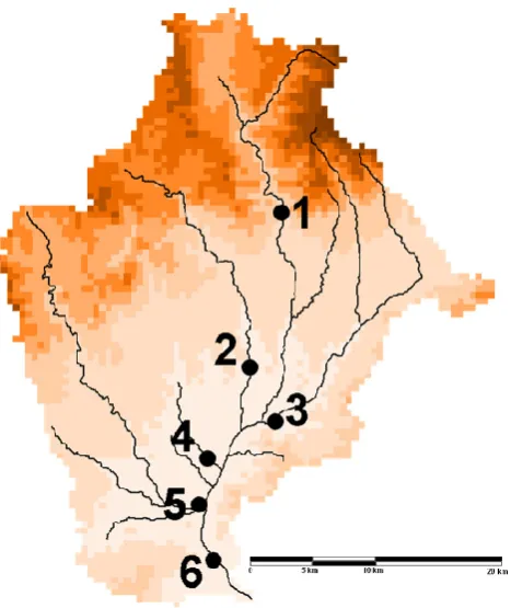
Fig. 1. Location map of Catalonia with superimposed relief and
boundary information, together with SAIH (ACA) and XEMA (SMC) raingauge networks.
wherevh(t) [m s−1] is the hillslope velocity at timetandKv is a parameter.
The model captures the main features of runoff generation processes in a watershed, while maintaining computational efficiency for real-time use.
3 Case studies and data
Catalonia is a region situated in the northeast corner of the Iberian Peninsula. Due to its proximity to the warm Mediter-ranean Sea and its complex orography, with several mountain ranges parallel to the coastline (Fig. 1), the presence of at-mospheric instability usually produces intense precipitation events during the summer and autumn seasons (Llasat et al., 2003). These heavy rainfall phenomena caused 217 floods over Catalonia from 1901 to 2000, of which more than 59 % were flash flood events (Barnolas and Llasat, 2007). The hy-drologic timescale of most watersheds is on the order of a few hours, and flash floods develop rapidly during the early autumn season and suddenly inundate urban streams, putting citizens at high risk.
Fig. 2. Location of the river gauging stations within the Besos
basin: 1-Garriga; 2-Llic¸a; 3-Mogent; 4-Mogoda; 5-Montcada; 6-Gramenet.
recent decades. After two catastrophic floods in Spain in 1982, considerable investment was devoted to monitoring the catchments for hydrological purposes. It is now instru-mented by several telemetered rain and streamflow gauges from SAIH (Automatic System of Hydrological Information) of the Catalan Water Agency (ACA, hereinafter) to a river park built in the river mouth to mitigate flood impacts.
The present work analyses four flash flood events with great social impact (Llasat et al., 2008) that were studied within the framework of the FLASH project (Price et al., 2011). The most relevant rainfall amounts for these cases are detailed in Table 1. For each case, rainfall amounts over the Bes`os Basin higher than 46 mm were recorded. The peak 5-min intensities during these events range from 80 mm h−1 to 135 mm h−1.
[image:4.595.52.286.60.338.2]The available ground rainfall data come from two differ-ent networks. The SAIH rain gauge network of the ACA is composed of 126 tipping-bucket automatic rain gauges cov-ering an area of about 16 000 km2called the Internal Basins of Catalonia (IBS) (Fig. 1). The precipitation is accumu-lated and recorded every 5 min. In this study, all of the 5-min series were subject to data quality control (Ceperuelo and Llasat, 2004). The second network, called XEMA (Au-tomatic Weather Station Network) is supported by the Cata-lan Meteorological Service (SMC, hereinafter) and is com-posed of 158 rain gauges and covers all of Catalonia (around
Table 1. Rainfall amount and intensity for the four study events
over the entire domain of Catalonia and over the Bes`os Basin.
Max. rainfall Max. rainfall amount (mm) intensity (mm/h) Data Catalonia Bes`os Catalonia Bes`os 2/08/2005 57.1 55.0 117.6 117.6 11–13/10/2005 348.2 81.7 129.6 108.0 13–15/11/2005 148.1 46.4 118.8 80.4 12–14/09/2006 266.1 117.6 249.6 135.6
32 114 km2). This network records the precipitation in two different temporal intervals. There are 47 stations that accu-mulate the precipitation every 30 min, while the remaining 111 stations have one-hour temporal resolution.
An straightforward merging of both networks produces a loss in temporal resolution (1 h) and a density of about 1 rain gauge per 100 km2, which is insufficient to reproduce the spatial pattern of most storms (Corral et al., 2001). Con-sequently, radar information is essential to simulate flash floods. In this work, the ACA network was used to com-pute the new Z/R relationship, whereas the SMC network was used to verify the results.
The radar rainfall estimation was implemented using data from the SMC radar network, which covers an area of 53 000 km2 over Catalonia and its surroundings. This net-work is made up of three C-band Doppler radars; a new radar was inaugurated in September 2008 but was not used in this study. The most important characteristics of the composed CAPPI imagery are the spatial resolution (2×2 km2), time resolution (6 min) and vertical resolution (1 km) from 1 km to 10 km of altitude (10 levels). The CAPPI are calculated by means of the IRIS program, which is based on the linear interpolation of the range to the selected heights in spheri-cal coordinates, with a correction for the Earth curvature to preserve data quality. The radar imagery was corrected using SMC by first passing a filter to remove ground clutter (Bech et al., 2003). A second filter was applied to remove the inter-ference between radars (no data in radar location) and from other non moving targets, such as a wind power plant.
[image:4.595.310.548.98.192.2]4 Methodology
The proposed methodology was used to perform a sensitiv-ity analysis of the rainfall time resolution, on the results of a hydrologic model in a flash-flood prone basin. As a dis-tributed hydrologic model is selected to better incorporate spatial variations of rainfall in time, spatially distributed rain-fall maps for different time resolutions were obtained from the 6-min weather radar data. The calibrated hydrologic model was run taking these estimated rainfall maps as in-put to determine the time resolution that best represents the hydrological behaviour of the basin.
The methodology is divided into two parts. The first part involves the estimation of the radar rainfall maps for different time resolutions. The second part concerns the probabilistic calibration of the RIBS hydrologic model and the sensitivity analysis of the rainfall time resolution to the results of the calibrated RIBS model.
4.1 Radar rainfall estimation
4.1.1 Method to calculate Z/R relation
In a previous work (Atencia et al., 2008), a large number of Z/R relations were tested for four selected heavy rainfall events. That study showed that radar-based rainfall data un-derestimated by approximately 18 % (56 mm), as compared to rain gauge measurements. Consequently, the results were not suitable for hydrological purposes.
To address the issue of QPE, a Z/R relation was obtained by applying the WPMM. This method (Rosenfeld et al., 1994) is based on matching the unconditional probabilities of rainfall and reflectivity. Obviously, point measures from radar and rain gauges are plagued by timing and spatial er-rors. Many of the timing and geometrical errors can be eliminated by applying the probability matching method us-ing synchronous time series (Rosenfeld et al., 1993). This is achieved by matching rain-gauge intensities to radar re-flectivities taken only from small windows centred over the gauges in time and space. Zawadzki (1975) has shown that both the window area (A), in km2, and the spread of the rain-gauge measurement in time (T), in h, are related as follows:
T=1
3· A12
V (5)
[image:5.595.311.547.62.259.2]whereV [km h−1] represents the horizontal velocity of the rainfall/storm-cell system. Atlas et al. (1990) and Rigo (2004) reported a climatic horizontal velocity of convective rainfall area of about 20 km h−1. Thus, a rain gauge time concentration of 6 min is obtained by applying this formulae (Eq. 5) for a 3×3 pixel window. In this study, the SAIH rain gauge data has a time resolution of 5 min. To ensure an op-timal correlation between both radar and rain gauge rainfall measurements (Rosenfeld et al., 1994), the solution is work with a temporal window of 30 min, which is a time interval
Fig. 3. Radar window example. Square window of 3×3 pixel di-mension is centered over a rain gauge (red cross).
that is greater than the optimal value. To solve this problem the following procedure has been applied:
– First, a radar window (3×3 pixels) around the rain gauge is built (Fig. 3).
– Second, each reflectivity’s independent window for ev-ery period of 30 min is taken from evev-ery pixel (45 in total) coming from five radar windows of each 6-min radar image (Fig. 4b)
– Third, 5-min rainfall intensity for each rain gauge is ac-cumulated in order to obtain rain gauge window for each period of 30 min (Fig.4a)
(a) Example of an independent rainfall window dataset:
Evolu-tion of 5-min rainfall rate for a period of 30 min.
(b) Example of a single independent reflectivity window
[image:6.595.65.531.62.234.2]dataset: 6-min reflectivities for a period of 30 min (5 radar im-ages) and for the nine pixels comprising a window.
Fig. 4. Examples of a rain gauge (a) and weather radar reflectivity (b) independent window.
(a) (b)
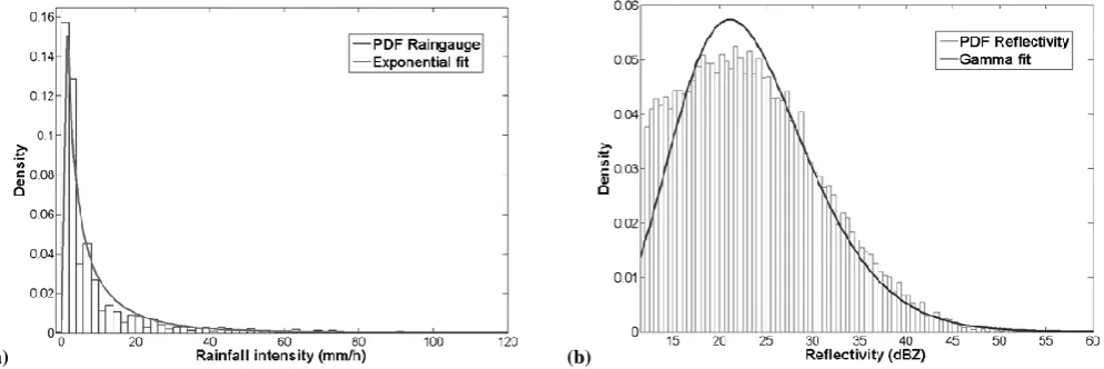
Fig. 5. The left picture (a) shows a density histogram of a random sub-sample of 25 % of the overall population of rain gauge data and the
Exponential pdf fit. The right one (b) shows density histogram for radar data window and Gamma pdf fit.
Adapting the Z/R relationship to different rain types within a given storm or event seems to be a promising way to improve radar QPE (Lee and Zawadzki, 2005). Rosenfeld et al. (1995) improved the accuracy of WPMM-estimated rainfall by means of objective classification criteria based on parameters such as freezing level or bright-band frac-tion. In the present work, the classification criteria developed by Biggerstaff and Listemaa (2000) were performed within a 3-D scheme, to recognise convective/stratiform areas (see also Steiner et al., 1995). This algorithm distinguishes be-tween convective and stratiform areas according to reflectiv-ity thresholds and gradients between different CAPPI lev-els, which were regionalised to Catalonia by Rigo and Llasat (2004). According to this methodology, in the present study, each different subset of every window was counted in differ-ent groups. Therefore, for the same rain gauge intensity
win-dow, two radar reflectivity windows are set. This approach to the classification criteria results in an ambiguous rain gauge probability distribution function. The ambiguous relation be-tween the intensity and rain type should be subsequently cal-culated as two independent unambiguous datasets.
[image:6.595.53.550.306.472.2](a) Division of the first image into templates (solid lines) and
search area (dashed line) corresponding to the central template.
(b) Vector indicating where in the second image the centre of
[image:7.595.65.234.63.284.2]the window (dotted line) closest to the original template (solid line) lies.
[image:7.595.304.474.112.283.2]Fig. 6. Example of templates in the second image for the cross-correlation technique and the displacement vector obtained. Both pictures, (a) and (b), are extracted from Dransfeld et al. (2006).
Fig. 7. Real example of radar rainfall disaggregation. In the above example 3×3 templates are shown in each image. The original resolution is 6 min and the cross-correlation advection results in a 1 min resolution.
4.1.2 Advection correction
The temporal sampling effect of radar observations can lead to significant errors in the estimated accumulated rainfall as shown in several studies (Liu and Krajewski, 1996; Fabry et al., 1994). To correct for this source of error, Anagnos-tou and Krajewski (1999) proposed an advection correction method based on cross-correlation maximisation (Rinehart and Garvey, 1978). This procedure can be applied not only to correct for these type of sampling errors, but also to increase the time resolution. For this reason, instead of calculating the cross-correlation coefficient between the two whole im-ages, the first image is divided into a number of template tiles (Fig. 6a). Each template window will be searched for in the second image using a search window (dashed line in Fig. 6a and 6b), whose size depends on the maximum storm speed that is expected between two sequential images. In the
present work, this technique was used to obtain the advective displacement vector (vector in Fig. 6b). This displacement (p,q)indicates a storm or cell movement (Dransfeld et al., 2006).
Once the advective displacement vector has been obtained by this method, a shape morphology transformation is per-formed by means of temporal weights based on a more com-plex shape transformation (Turk and O’Brien, 2005). Both the first,A(x,y), and second rainfall fields,B(x,y), are inter-polated by means of the computed velocity to the same tem-poral interval. Then, the value of rainfall at location(x,y) and timet,R(x,y,t ), is calculated as the temporal-weighted sum of the two images as shown in the next function: R(x,y,t )= 1
T2· X n
(T−t )·A(t )e +t·B(t )e o
[image:7.595.56.549.363.455.2]Fig. 8. Superposition of radar pixels over DEM grid over a small
domain of areaA2. The highlighted grey DEM grid pixel is used as example of mismatching between the two grids.
where the transformed fieldsA(x,y,t )e andB(x,y,t )e are cal-culated by the functions
e
A(x,y,t )=Ahx− t
T ·c·cosθ,y− t
T ·c·sinθ i
(7)
e
B(x,y,t )=B h
x+T−t
T ·c·cosθ,y+ T−t
T ·c·sinθ i
(8) whereAandB are consecutive radar rainfall fields. cis the advective velocity [km h−1] andθis the displacement angle. T [h] represents the original time resolution of radar andt [h] is time within the time intervalT.
The template size selected is 10×8 pixels, whereas the search window for the second image is 16×14 pixels. This size was calculated by assuming a maximum storm movement lower than 140 km h−1, following the works of Steinacker et al. (2000) and Rigo (2004). Figure 7 shows the downscaling from 6 min to 1 min.
4.1.3 Rainfall data into RIBS hydrological model
The RIBS model requires that rainfall input data be mapped to the rectangular grid of the DEM. As radar images and
DEM resolutions are different and may correspond to dif-ferent projections, a preliminary treatment of radar images is required.
The main step is an interpolation to downscale the radar resolution grid (2 km×2 km) to the DEM resolution (200 m×200 m). The easiest and quickest way is to perform an ordinary linear interpolation, but this methodology does not exactly preserve the total amount of precipitation over the whole domain due to mismatching grids (Fig. 8). To avoid this, another procedure was developed in the present work. As shown in Fig. 8, some DEM grid cells are divided into two different reflectivity parts (grey cell). The main purpose of the new procedure is to preserve the total areal precipita-tion amount, which is achieved by an area-weighted interpo-lation. This could be formulated in a general way as follows:
RDj=
X
i∈Ij SjiRi
X
i∈Ij
Sji (9)
where RDj is rainfall intensity in DEM cellj,Ri is rainfall
intensity in radar celli,Ij is the set of radar cells that cover
DEM cell j andSji is the area of DEM cellj covered by radar celli.
Once rain rated for every cell of the whole domain has been calculated by this area-weighted interpolation, the Bes`os Basin shape is cut out from the high resolution rainfall image.
4.1.4 Radar rainfall validation
To evaluate the accuracy of the radar rainfall estimation, three error indexes are calculated. The first one is the log ratio bias (Eq. 10), which is a relative error and provides in-formation about the total amount of precipitation:
log ratio bias=log· P
Ri
P Pi
(10) The second is the Root Mean Square Error (RMSER; Eq. 11)
[mm], which determines the accuracy of the estimation for each individual rain gauge.
RMSER=
s P
(Ri−Pi)2
n (11)
The third is the Mean Error (MER; Eq. 12) [mm], which
de-fines whether the rainfall is under/over-estimated. MER=
P
(Ri−Pi)
n (12)
Here, Ri and Pi are the rainfall amount at locationi
4.2 Hydrological modeling
4.2.1 Selection of rainfall time resolutions
Spatially distributed precipitation maps can be constructed for each event by summing the new advected 1-min radar rainfall maps to a given resolution. A set of time resolutions must be selected to perform the analysis.
The required minimum time resolution of rainfall for Mediterranean regions can be estimated as a function of the basin area (Eq. 13), taking into account that time resolu-tions higher than 3 min only become relevant for basin areas smaller than 100 ha (1 km2) (Berne et al., 2004).
1t=0.75·S0.3 (13)
where1tis the required minimum time resolution [min], and Sis the basin area [ha].
4.2.2 Probabilistic calibration
The distributed RIBS model was calibrated using a prob-abilistic approach based on a multiobjective calibration methodology, since both different aspects of the hydrograph and the uncertainty in the hydrologic model estimations may be taken into account. The calibration result is a pdf for each calibrated model parameter (Mediero et al., 2011).
The probabilistic calibration methodology can be sum-marised as follows. First, a sensitivity analysis was per-formed over the global parameters of the RIBS model, since the local parameters, asK0n, were estimated from the soil
types in the basin prior to the calibration. As model input ob-served rainfall data in the first event at a 15 min time resolu-tion was used, and model parameter values were randomised from uniform distributions. A modification of the Gener-alised Sensitivity Analysis (GSA) methodology proposed by Freer et al. (1996) was applied. This analysis showed that the most influential parameters in the model output are as follows: the rate of variation of the hydraulic conductivity in depth (f), the soil anisotropy coefficient (α), the ratio of hillslope flow velocity to channel flow velocity (Kv) and the coefficient of the law that relates hillslope flow velocity to discharge in the basin outlet (Cv).
Second, the proper calibration methodology was per-formed over the first three recorded events for each rain-fall time resolution. A large set of synthetic hydrographs was generated by repetitive simulations of the RIBS model; these simulations generated randomised sets of values for the most influential model parameters, which were identified in the first step. Hydrological model outputs highly depend on the initial basin conditions. Therefore, the antecedent moisture content in the basin is an input of the RIBS model and it was estimated from rainfall and temperature data in the days before the beginning of each flood event. As the model utilisation is the prediction of flash floods, the Root Mean Square Error (RMSE; Eq. 14), Mean Absolute Er-ror (MAE; Eq. 16) and Nash-Sutcliffe Efficiency Coefficient
(NSE; Eq. 17) were selected as objective functions to con-duct the multiobjective calibration.
RMSE= v u u t 1 Ts Ts X
t=1 Qt
o−Qts 2
(14)
MEH= Ts X
t=1
Qto−Qts (15)
MAE=
Ts X
t=1
| Qto−Qts|
(16)
NSE=1−
Ts P
t=1
[Qto−Qs]2
Ts P
t=1 [Qt
o−Qo]2
(17)
whereQtois the observed discharge at timet,Qts is the sim-ulated discharge at timet,Qois the mean of observed dis-charges,Qsis the mean of simulated discharges andTsis the total number of time steps.
In a multiobjective calibration, no single solution can min-imise all of the objective functions at the same time (Gupta et al., 1998). Therefore, the Pareto solutions were identified to determine the set of non-inferior solutions (Yapo et al., 1998). Each calibrated model parameter was represented by a pdf fitted from the set of Pareto solutions for the three calibration events. The distribution functions that best fit the variability of each parameter were identified by means of traditional goodness-of-fit tests, i.e. Chi-Squared test and Kolmogorov-Smirnov test.
4.2.3 Sensitivity analysis of the rainfall time resolution The result of the probabilistic calibration of the RIBS model is a pdf for each parameter, which represents the parameter’s variability. Therefore, the result of the model calibration is not a single hydrograph, but an ensemble distribution hydro-graphs. This ensemble is obtained by the randomisation of the model parameter values based on the calibration results. The number of hydrographs used to analyse the importance of time resolution must be large enough to reach the stabilisa-tion of the model results. The required number of simulastabilisa-tions was defined through a sensitivity analysis, which established that 200 model simulations were required to obtain reliable results.
A sensitivity analysis of the rainfall time resolution was performed for the last observed event. Differences between the simulated set of hydrographs and the observed hydro-graph were quantified by four measures. RMSE and Mean Error (MEH) were selected to measure the accuracy of the
simulations (Eq. 14–15).
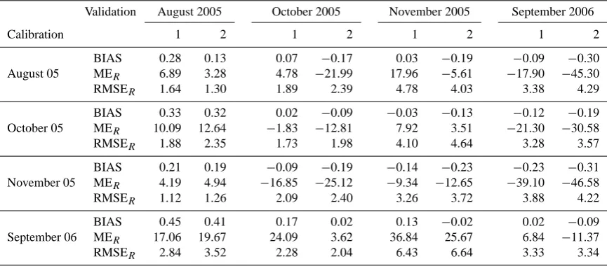
Table 2. Validation results for the eight Z/R relationships in each of the four study cases. The numbers in the second row represent the pdf
fitting method, being 1 exponential-Gamma and 2 for the Kernel smoothing density function.
Validation August 2005 October 2005 November 2005 September 2006
Calibration 1 2 1 2 1 2 1 2
BIAS 0.28 0.13 0.07 −0.17 0.03 −0.19 −0.09 −0.30 August 05 MER 6.89 3.28 4.78 −21.99 17.96 −5.61 −17.90 −45.30 RMSER 1.64 1.30 1.89 2.39 4.78 4.03 3.38 4.29
BIAS 0.33 0.32 0.02 −0.09 −0.03 −0.13 −0.12 −0.19 October 05 MER 10.09 12.64 −1.83 −12.81 7.92 3.51 −21.30 −30.58
RMSER 1.88 2.35 1.73 1.98 4.10 4.64 3.28 3.57
BIAS 0.21 0.19 −0.09 −0.19 −0.14 −0.23 −0.23 −0.31 November 05 MER 4.19 4.94 −16.85 −25.12 −9.34 −12.65 −39.10 −46.58
RMSER 1.12 1.26 2.09 2.40 3.26 3.72 3.88 4.22
BIAS 0.45 0.41 0.17 0.02 0.13 −0.02 0.02 −0.09 September 06 MER 17.06 19.67 24.09 3.62 36.84 25.67 6.84 −11.37
RMSER 2.84 3.52 2.28 2.04 6.43 6.64 3.33 3.34
of the Nash-Sutcliffe global efficiency index (R2 (MQ0.5); Eq. 18), which measures the utility of the median, instead of the mean, as a forecast (Xiong and O’Connor, 2008).
R2(MQ0.5)=1.0−
Ts P
t=1
[Qto−MQt0.5]2
Ts P
t=1 [Qt
o−Qo]
(18)
where MQt0.5is the median of simulated discharges at timet. The predictive capability of the calibrated model was quantified by the Containing Ratio (CR; Eq. 19), which mea-sures the number of observations that fall within the predic-tion interval linked to a given confidence level (Montanari, 2005).
CR(α)= P
I[Qto] Ts
(19) whereI[Qto]is equal to 1 if the observed discharge at time t holds between the confidence interval, andαis the confi-dence level, which was set at 10 %.
5 Results
5.1 WPMM methodology
The four selected heavy rainfall events were produced by very different meteorological events. For this reason, the cal-ibration method previously presented was applied for each case such that eight Z/R relations were obtained: two fitting methods for each of the four case studies. In Table 2, er-ror indices are presented for the eight functions, which are compared for every case using the total event amount in the comparison.
Regarding the comparison of both methodologies, it can be observed that a parametric fit (exponential-Gamma) im-proves results compared to a non-parametric fit (Fig. 9). The left box plot for a given fitting methodology, represents the results for the Z/R obtained for the same study case, whereas the right box plot shows the Z/R results computed for the three other case studies. The log ratio bias and the RMSER
show better results for both box plot regarding the mean and the interquartile range. It can be observed that, in general, best results are obtained for the left box plots. Nevertheless, as the results show, also for the other three events calibrated fits achieve accurate precipitation estimations.
A comparison between both methodologies shows that the parametric fit improves the range of applicability of the new Z/R relationship. It can be observed in Fig. 10 that the SD is higher for the tails of the non-parametric Z/R relation (Fig. 10a) than for the parametric Z/R relation (Fig. 10b). This is caused by the scarcity of values in the tails of the probability distribution function for the reflectivity and high intensity rainfall values. The parametric fit does not have this problem because it has only two parameters to compute, and this computation gives more weight to the central values of the distribution.
5.2 Advection correction
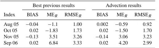
Table 3. Comparison of results before and after applying the
advec-tion correcadvec-tion.
Best previous results Advection results
Index BIAS MER RMSER BIAS MER RMSER
Aug 05 −0.04 −1.1 1.00 0.002 −0.59 0.92
Oct 05 0.02 −1.83 1.73 0.02 −1.50 1.70
Nov 05 −0.13 3.51 3.26 −0.14 3.06 3.23
[image:11.595.48.307.96.174.2]Sep 06 0.02 6.84 3.33 0.02 4.20 2.99
Table 4. Basin area (km2), length of the main watercourse (km), slope between maximum and minimum elevation (m/m), time of concentration by the Kirpich formula (h) and required minimum time resolution of rainfall in Mediterranean regions (min) of Bes`os basin stations.
Station Area (km2) L (km) S(m/m) tc(h) 1tmin[min]
Mogoda 111 31.83 0.026 3.87 12.3
Llic¸a 146 38.71 0.023 4.73 13.3
Garriga 151 26.41 0.026 3.36 13.5
Mogent 182 36.66 0.032 3.99 14.2
Montcada 221 43.24 0.015 6.15 15.1
Gramenet 1012 63.45 0.015 8.26 23.8
The impact of the advection can be observed in Fig. 11. The maximum values and the shape of the rainfall field has changed for this specific example. Regarding the improve-ment in the hourly accumulated rainfall, Fig. 12 compares the log ratio bias and the RMSERof the QPE before and
af-ter applying the advection correction technique. 5.2.1 Selection of rainfall time resolutions
The minimum time resolution for the gauging stations in the Bes`os Basin calculated using Eq. (13) are included in Ta-ble 4. It can be seen that they are within 12 to 24 min. There-fore, the calibration of the RIBS model was performed for six time resolutions: 30, 24, 18, 15, 12 and 6 min. Resolutions higher than 6 min were not considered because this greatly increases the computation time of the RIBS model. More-over, these time resolutions are not relevant for the basin ar-eas considered in the Bes`os Basin.
5.3 Hydrologic model calibration
[image:11.595.48.287.262.343.2]The distributed RIBS model was calibrated in the Bes`os Basin with the first three observed events. The basin shape and the locations of the gauging stations are shown in Fig. 2, and their basic properties are presented in Table 4. The model was calibrated using data from the Gramenet station, very near the basin outlet. Spatially distributed precipitation maps were constructed for each event by summing the new ad-vected radar rainfall estimation for 30, 24, 18, 15, 12 and 6 min. The antecedent moisture content was used as an input
Fig. 9. Box-plot of both fitting techniques (parametric and
non-parametric) for the log ratio bias and the RMSER. The left
box-plot for a given fitting methodology represents the results for the Z/R obtained for the same study case whereas the right box plot is the results obtained for the Z/R computed by the three other case studies.
in the RIBS model from rainfall and temperature data in the days before the flood event.
The calibration methodology was conducted for each rain-fall time resolution to take into account the fact that some hydrological parameters may be dependent on the time scale. The calibration results are summarised by the main statistics of the distribution of parameter values for each time resolu-tion (Table 5).
5.4 Sensitivity to precipitation time resolution
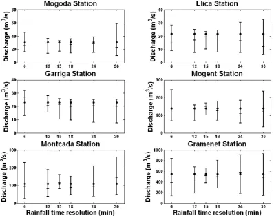
A sensitivity analysis of the rainfall time resolution was car-ried out for the last event, at each of the six gauging stations: Llic¸a station on the Tenas River, Montcada Station on the Ripoll River, just upstream of its confluence with the Bes`os River, Gramenet Station on the Bes`os River, very near the basin outlet, Garriga Station on the Congost River, Mogent Station on the Mogent River and Mogoda Station on the Cal-das River (Fig. 2).
A set of 200 simulated hydrographs was generated for each time resolution. These simulated hydrographs were compared with the observed flows for each gauge as de-scribed in Sect. 4.2.3; the results obtained are presented in Table 6 and Figs. 13 and 14.
(a) Non-parametric (b) Parametric
Fig. 10. The new Z/R relation (solid middle line), as obtained from WPMM for the full dataset. The broken lines represent plus and minus
one standard deviations from the Z/R when calculated by population from 1 % to 25 % sub-samples. The left example (a) is the new Z/R relation obtained by non-parametric fitting whereas the right one (b) correspond to the parametric fit.
(a) Before advection correction (b) After advection correction
Fig. 11. Comparison between non-advected (a) and advected (b) accumulated rainfall field.
of 12, 15 and 18 min. In general, both the width of the con-fidence intervals and the distances between the median and the observed peak increase as the rainfall time resolution de-viates from these values, reaching the maximum at the most extreme time resolutions, i.e. 6 and 30 min. The largest devi-ations of the median from the observed peak at most stdevi-ations are also at 6 and 30 min.
The results obtained for the four validation measures are shown in Fig. 14. To allow for the comparison among gauges, RMSE and MEH were standardised by the observed
peak discharge. As shown in Fig. 14a, the minimum RMSE is reached at all stations for 15 min resolution, except for the Mogoda station. The model performance is maintained for time resolutions below 12 min but decreases sharply for time
resolutions above 18 min in the case of the smaller stations, Mogoda, Llic¸a and Garriga. This finding shows that time res-olutions coarser than 15 min worsen the hydrological results for the basins with smaller areas.
[image:12.595.66.531.311.506.2]Fig. 12. Validation results for the September 2006 event before and after applying the advection correction.
Fig. 13. Validation results for the peak discharge as a function of time resolution, at all station locations. The observed peak discharge is
plotted as a solid circle, 5 % and 95 % percentiles are plotted as vertical bars and the median is plotted as a horizontal dash.
Gramenet, Montcada and Mogent Stations clearly reach the bestR2(MQ0.5)for a time resolution of 15 min. Mogoda and Llic¸a Stations reach the maximum for 15 min, but there are no large differences from the result for 12 min. Garriga reaches the maximum for 12 min. These results indicate that the larger basins produce better results for a time resolution
of 15 min and that the smaller basins produce better results for a higher time resolution closer to 12 min.
[image:13.595.101.500.268.581.2](a) (b)
[image:14.595.54.552.61.391.2](c) (d)
Fig. 14. Validation measures plotted versus rainfall time resolution for all stations. (a) Root Mean Square Error (RMSE), standardized by
observed peak discharge (b); absolute value of Bias (ME), standardized by observed peak discharge. (c) ash-Sutcliffe global efficiency index
R2(MQ0.5). (d) Containing Ratio for a confidence level of 10 %[CR(10 %)].
Table 5. Summary of calibration results for each parameter for all time resolutions. Table shows mean value (µ) and standard deviation (σ) of the parameter distribution.
Parameter
Time resolution log10(f) [mm−1] α[−] Kv[−] Cv[m h−1]
(min) µ σ µ σ µ σ µ σ
6 −3.05 0.92 41.6 25.8 10.1 2.82 4680 1654 12 −2.15 0.71 48.6 28.9 10.9 1.80 4643 1220 15 −2.63 0.68 53.4 27.1 11.3 2.15 4397 1313 18 −2.30 0.51 48.9 30.6 10.7 1.75 4563 1818 24 −2.32 0.29 44.0 28.8 10.1 1.95 4593 1655 30 −2.65 0.69 50.6 24.4 11.1 2.77 3415 1439
as the time resolution increases. The best results are achieved at 15 min resolution, but the results for 12 min are worse than those for 18 min. This finding indicates that the results for the larger basins give worse results at time resolutions higher than 15 min. In the case of smaller basins, there are not relevant differences between the results of time resolutions within 12 and 15 min.
[image:14.595.141.454.485.604.2]Table 6. Validation results for the selected river gauging stations.
Time resolution
Gauge station Measure 30 min 24 min 18 min 15 min 12 min 6 min
Llic¸a
RMSE 16.212 11.546 7.577 3.586 3.911 4.142 Bias −12.072 −8.843 −5.939 −1.143 0.325 1.568
R2(MQ0.5) 0.315 0.333 0.392 0.416 0.387 0.360 CR (10 %) 0.254 0.319 0.337 0.365 0.440 0.312
Montcada
RMSE 24.398 19.708 16.718 13.993 14.893 16.003 Bias −13.842 −8.157 −5.891 0.548 2.744 5.747
R2(MQ0.5) 0.330 0.376 0.474 0.528 0.474 0.391 CR (10 %) 0.522 0.616 0.693 0.789 0.614 0.523
Gramenet
RMSE 85.530 71.237 68.725 60.656 64.435 68.516 Bias −43.843 −25.817 −14.795 10.658 15.365 25.131
R2(MQ0.5) 0.398 0.421 0.438 0.521 0.432 0.356 CR (10 %) 0.498 0.520 0.539 0.686 0.592 0.504
Garriga
RMSE 9.726 8.003 7.278 3.108 3.736 4.741 Bias −6.669 −5.142 −3.385 0.005 1.049 1.644
R2(MQ0.5) 0.290 0.307 0.321 0.347 0.382 0.316 CR (10 %) 0.284 0.308 0.381 0.490 0.395 0.201
Mogent
RMSE 24.586 21.422 15.130 14.257 15.020 16.460 Bias −7.331 −4.393 −2.524 −1.789 0.214 4.803
R2(MQ0.5) 0.208 0.375 0.472 0.545 0.443 0.346 CR (10 %) 0.304 0.389 0.482 0.614 0.589 0.485
Mogoda
RMSE 11.192 7.138 6.234 5.206 4.505 6.213 Bias 7.599 4.100 3.295 2.201 −0.049 3.310
R2(MQ0.5) 0.243 0.388 0.419 0.443 0.438 0.373 CR (10 %) 0.284 0.341 0.424 0.543 0.468 0.435
a threshold for a basin area of 150 km2. Basins with areas below this threshold produce better results with a time reso-lution of 12 min, causing the model performance to decrease sharply as the time resolution decreases. Basins with areas higher than 150 km2achieve better results with a time reso-lution of 15 min.
These results indicate that 15 min is the best rainfall time resolution for basins larger than 150 km2in the Bes`os Basin and 12 min is the best resolution for basins smaller than 150 km2. These time resolutions provide a good represen-tation of the rainfall characteristics of the Bes`os River basin as well as allow for a good simulation of the hydrological processes that occur in the area.
6 Discussion
Distributed hydrological models improve the simulation of convective rainfall events, as they can accept spatially dis-tributed rainfall maps as input data. In this study, an effort was made to couple radar data with a distributed hydrologic model to simulate flash-flood events recorded in Catalonia.
This contribution provides a good example of the numer-ous problems that exist in QPE. First, the traditional Z/R power-law relationships have not worked well when applied to the selected cases. It is difficult to determine with certainty whether this problem might be associated with poor calibra-tion or maintenance of the radar network, or with the atten-uation caused by heavy precipitation. To obtain a suitable QPE, a Window Probability Matching Method (WPMM) and an advection correction were applied in this work.
functions used were a gamma function for reflectivity and an exponential function for rainfall intensity. Comparing both methodologies, the parametric function provides an increase in lower reflectivity values and a decrease in higher values, whereas the non-parametric methodology produces a similar shape, though it is displaced to the right, which causes the rainfall intensity to increase for all reflectivity values. The second correction made by WPMM non-parametric method-ology could be related to the underestimation of the reflectiv-ity due to the power parameter calibration or attenuation due to heavy rainfall.
Taking into account the improvement that involves a con-vective/stratiform distinction, two Z/R relations are obtained. This new QPE method produces better results for the log ratio bias, which indicates a more accurate reproduction of the total rainfall recorded. Furthermore, the new WPMM Z/R relation shape is less convex than the previous one. Ac-cordingly, this approach should be useful for obtaining better QPE results if more in-depth rain regime research was per-formed.
After that, an advection correction was applied to correct the rainfall amount. This correction was based on the hy-pothesis that rainfall intensities continuously vary in space. This method is applied by several meteorological services to accumulate rainfall over a period of one hour. In the present work, this technique was applied to every six radar rainfall fields with two objectives. The first was to improve the total rainfall estimation; the second was to increase the temporal resolution to feed the hydrological model. By applying this method, the root mean square error decreased, although the bias did not show this behaviour. The cause of this could be the significance of each improvement. The root mean square error is more closely related with point errors, whereas the bias is mainly related to the entire rainfall field.
Comparing the results obtained in the literature for the Z/R relations (Atencia et al., 2008) with the results of the com-bined application of both methodologies, the RMSER has
been reduced by up to 40 % and log ratio bias between 75 % and 95 %. These accurate results allow us to map the radar rainfall information to the rectangular grid of the DEM by an area-weighted interpolation.
Once a more accurate rainfall field was obtained for each 6-min interval, it was taken as input data for the hydrologic model. Due to the fact that the calibration of distributed hy-drological models is strongly dependent on the time resolu-tion of rainfall data, the advecresolu-tion correcresolu-tion method based on a cross-correlation technique was applied to implement a temporal disaggregation at several time resolutions (30, 24, 18, 15, 12, 6 and 2 min). Time resolutions higher than 6 min lead to both unaffordable computation times for operational hydrological forecasting and irrelevant time resolutions for the gauging stations in the Bes`os River Basin. Accordingly, only the six highest time resolutions were compared.
A probabilistic calibration methodology was applied to three flood events to obtain the pdf that best represent the
variability of each model parameter. A sensitivity analysis of the rainfall time resolution was performed for the last event. This sensitivity analysis showed that basins with areas be-low 150 km2provide better results with a time resolution of 12 min, and basins with areas higher than 150 km2achieve better results with 15 min of time resolution. This result may be influenced by the fact that the model was only calibrated for the global outlet at Gramenet. An individual calibration of each of the smaller basins might lead to better overall model performance and would probably yield a lower opti-mum time resolution in smaller basins. The selected rainfall time resolutions compare well with the results presented by (Berne et al., 2004), who studied urban basins up to 100 km2 and found a strong relationship between basin size and the minimum required rainfall spatial and temporal resolutions, suggesting a rainfall minimum temporal resolution of 12 min. For the optimum time resolution of 15 min, an RMSE av-erage improvement of 16 % was obtained for all sub-basins analysed when compared to the 6 min time resolution case, which produced values larger than 10 % for all individual basins. The results for other basins could vary across the Mediterranean due to the dependence of the basin response on other characteristics not analysed in this work, such as geomorphology, geology and vegetation.
7 Conclusions
The goal of this study was to perform a sensitivity analy-sis of rainfall time resolution on coupling radar data with a distributed hydrologic model to simulate flash-flood events recorded in Catalonia.
The first step was to obtain a methodology that improves the radar rainfall estimation. The results shows that the appli-cation of a WPMM, to compute a new Z/R relation, together with an advection correction, represents a good improvement in radar rainfall estimation.
The advection correction technique was applied to imple-ment a temporal disaggregation at several rainfall time reso-lutions (from 30 to 6 min). After a probabilistic calibration of the hydrological model, a sensitivity analysis of these rainfall time resolutions was performed.
The basins analysed in this work range from 100 to 1000 km2 and present an optimum time resolution between 12 and 15 min. This result proves that the highest available rainfall time resolution does not necessarily provide the best result in terms of the predictability of peak flow when the radar system is coupled with a distributed hydrologic model.
Acknowledgements. This research is supported by the Sixth
of Water) for the rainfall and stream flow data from the SAIH network. Additionally, the authors would like to thank CLABSA for the Bes`os Basin information.
Edited by: R. Uijlenhoet
References
Anagnostou, E. and Krajewski, W.: Real-time radar rainfall esti-mation. Part I: Algorithm formulation, Journal of Atmospheric and Oceanic Technology, 16, 189–197, doi:10.1175/1520-0426(1999)016<0189:RTRREP>2.0.CO;2, 1999.
Anquetin, S., Braud, I., Vannier, O., Viallet, P., Boudevillain, B., Creutin, J., and Manus, C.: Sensitivity of the hydrological re-sponse to the variability of rainfall fields and soils for the Gard 2002 flash-flood event, J. Hydrol., 394, 134–147, 2010. Arnaud, P., Bouvier, C., Cisneros, L., and Dominguez, R.: Influence
of rainfall spatial variability on flood prediction, J. Hydrol., 260, 216–230, doi:10.1016/S0022-1694(01)00611-4, 2002.
Atencia, A., Ceperuelo, M., Llasat, M., and Vilaclara, E.: A new non power-law Z/R relation in western Mediterranean area for flash-flood events, in: Proceedings of Fifth European Confer-ence on Radar in Meteorology and Hidrology (ERAD)., p. 14, Helsinki, Finland, 7, 2008.
Atlas, D., Rosenfeld, D., Wolff, D., Aeronautics, N., and Space Ad-ministration. Goddard Space Flight Center, Greenbelt, M.: Cli-matologically tuned reflectivity-rain rate relations and links to area-time integrals, J. Appl. Meteorol., 29, 1120–1135, 1990. Barnolas, M. and Llasat, M. C.: A flood geodatabase and its
clima-tological applications: the case of Catalonia for the last century, Nat. Hazards Earth Syst. Sci., 7, 271–281, doi:10.5194/nhess-7-271-2007, 2007.
Barnolas, M., Rigo, T., and Llasat, M. C.: Characteristics of 2-D convective structures in Catalonia (NE Spain): an analysis us-ing radar data and GIS, Hydrol. Earth Syst. Sci., 14, 129–139, doi:10.5194/hess-14-129-2010, 2010.
Bech, J., Codina, B., Lorente, J., and Bebbington, D.: The sensitivity of single polarization weather radar beam block-age correction to variability in the vertical refractivity gradient, J. Atmos. Oceanic Technol., 20, 845–855, doi:10.1175/1520-0426(2003)020<0845:TSOSPW>2.0.CO;2, 2003.
Bell, V. A. and Moore, R. J.: The sensitivity of catchment runoff models to rainfall data at different spatial scales, Hydrol. Earth Syst. Sci., 4, 653–667, doi:10.5194/hess-4-653-2000, 2000. Berne, A., Delrieu, G., Creutin, J., and Obled, C.: Temporal and
spatial resolution of rainfall measurements required for urban hy-drology, J. Hyhy-drology, 299, 166–179, 2004.
Biggerstaff, M. and Listemaa, S.: An improved scheme for convective/stratiform echo classification using radar reflectiv-ity, J. Appl. Meteorol., 39, 2129–2150, doi:10.1175/1520-0450(2001)040<2129:AISFCS>2.0.CO;2, 2000.
Bouilloud, L., Delrieu, G., Boudevillain, B., and Kirstetter, P.: Radar rainfall estimation in the context of post-event analysis of flash-flood events, J. Hydrol., 394, 17–27, 2010.
Carpenter, T. and Georgakakos, K.: Intercomparison of lumped versus distributed hydrologic model ensemble simulations on operational forecast scales, J. Hydrol., 329, 174–185, doi:10.1016/j.jhydrol.2006.02.013, 2006.
Ceperuelo, M. and Llasat, M.: La Precipitacion Convectiva en las Cuencas Internas de Catalunya, Revista del Aficionado a la Me-teorologıa, 23, 2004.
Corral, C., Sempere-Torres, D., and Berenguer, M.: A distributed rainfall runoff model to use in Mediterranean basins with radar rainfall estimates, in: 30 Conf. on Radar Meteor, pp. 6–8, 2001. Delrieu, G., Andrieu, H., and Creutin, J.: Quantification of
path-integrated attenuation for X-and C-band weather radar systems operating in Mediterranean heavy rainfall, J. Appl. Meteorol., 39, 840–850, 2000.
Dransfeld, S., Larnicol, G., and Le Traon, P.: The Potential of the Maximum Cross-Correlation Technique to Estimate Surface Currents From Thermal AVHRR Global Area Coverage Data, IEEE Geoscience and Remote Sensing Letters, 3, 508–511, doi:10.1109/LGRS.2006.878439, 2006.
Fabry, F., Bellon, A., Duncan, M., and Austin, G.: High resolution rainfall measurements by radar for very small basins: the sam-pling problem reexamined, J. Hydrol., 161, 415–428, 1994. Franco, M., S´anchez-Diezma, R., and Sempere-Torres, D.:
Improv-ing radar precipitation estimates by applyImprov-ing a VPR correction method based on separating precipitation types, in: Proceed-ings of Fifth European Conference on Radar in Meteorology and Hidrology (ERAD)., p. 14, Helsinki, Finland, 14, 2008. Freer, J., Beven, K., and Ambroise, B.: Bayesian estimation of
un-certainty in runoff prediction and the value of data: An applica-tion of the GLUE approach, Water Resour. Res., 32, 2161–2173, 1996.
Garrote, L. and Bras, R.: A distributed model for real-time flood forecasting using digital elevation models, J. Hydrol., 167, 279– 306, doi:10.1016/0022-1694(94)02592-Y, 1995a.
Garrote, L. and Bras, R.: An integrated software environment for real-time use of a distributed hydrologic model, J. Hydrol., 167, 307–326, 1995b.
Garrote, L., Molina, M., and Mediero, L.: Hydroinformatics in Practice: Computational Intelligence and Technological Devel-opments in Water Applications, chap. Learning Bayesian net-works from deterministic rainfall–runoff models and Monte-Carlo simulation, pp. 375–388, Springer, doi:10.1007/978-3-540-79881-1 27, 2007.
Gupta, H., Sorooshian, S., and Yapo, P.: Toward improved cali-bration of hydrologic models: Multiple and noncommensurable measures of information, Water Resour. Res., 34, 751–763, 1998. Haddad, Z., Short, D., Durden, S., Im, E., Hensley, S., Grable, M., and Black, R.: A new parametrization of the rain drop size distri-bution, IEEE Transactions on Geoscience and Remote Sensing, 35, 532–539, doi:10.1109/36.581961, 1997.
Hazenberg, P., Yu, N., Boudevillain, B., Delrieu, G., and Uijlen-hoet, R.: Scaling of raindrop size distributions and classification of radar reflectivity-rain rate relations in intense Mediterranean precipitation, J. Hydrol., 402, 179–192, 2011.
Kaplan, E. and Meier, P.: Nonparametric estimation from incom-plete observations, J. Am. Statistical Association, 53, 457–481, doi:10.2307/2281868, 1958.
Krajewski, W., Lakshmi, V., Georgakakos, K., and Jain, S.: A Monte Carlo study of rainfall sampling effect on a dis-tributed catchment model, Water Resour. Res., 27, 119–128, doi:10.1029/90WR01977, 1991.
ef-fects on rain estimation, J. Appl. Meteorol., 44, 241–255, doi:10.1175/JAM2183.1, 2005.
Liu, C. and Krajewski, W.: A comparison of methods for calcula-tion of radar-rainfall hourly accumulacalcula-tions, J. Am. Water Resour. Assoc., 32, 305–315, doi:10.1111/j.1752-1688.1996.tb03453.x, 1996.
Llasat, M., Rigo, T., and Barriendos, M.: The Montserrat-2000 flash-flood event: a comparison with the floods that have oc-curred in the northeastern Iberian Peninsula since the 14th cen-tury, Int. J. Climatol., 23, 453–469, doi:10.1002/joc.888, 2003. Llasat, M. C., L´opez, L., Barnolas, M., and Llasat-Botija,
M.: Flash-floods in Catalonia: the social perception in a context of changing vulnerability, Adv. Geosci., 17, 63–70, doi:10.5194/adgeo-17-63-2008, 2008.
Madsen, H.: Parameter estimation in distributed hydrological catch-ment modelling using automatic calibration with multiple ob-jectives, Adv. Water Resour., 26, 205–216, doi:10.1016/S0309-1708(02)00092-1, 2003.
Marchi, L., Borga, M., Preciso, E., and Gaume, E.: Characterisation of selected extreme flash floods in Europe and implications for flood risk management, J. Hydrol., 394, 118–133, 2010. Marshall, J. and Palmer, W.: The distribution of raindrops
with size, J. Atmos. Sci., 5, 165–166, doi:10.1175/1520-0469(1948)005<0165:TDORWS>2.0.CO;2, 1948.
Mediero, L., Garrote, L., and Martin-Carrasco, F.: A probabilis-tic model to support reservoir operation decisions during flash floods/Un modele probabiliste d’aide a la decision pour la ges-tion d’un reservoir lors de crues eclairs, Hydrol. Sci. J., 52, 523– 537, doi:10.1623/hysj.52.3.523, 2007.
Mediero, L., Garrote, L., and Mart´ın-Carrasco, F.: Probabilistic cal-ibration of a distributed hydrological model for flood forecasting, Hydrol. Sci. J., 56, 1129–1149, 2011.
Montanari, A.: Large sample behaviors of the generalized likeli-hood uncertainty estimation (GLUE) in assessing the uncertainty of rainfall-runoff simulations, Water Resour. Res., 41, W08406, doi:10.1029/2004WR003826, 2005.
Morin, E. and Gabella, M.: Radar-based quantitative pre-cipitation estimation over Mediterranean and dry climate regimes, J. Geophys. Res.-Atmospheres, 112, D20108, doi:10.1029/2006JD008206, 2007.
Morin, E., Enzel, Y., Shamir, U., and Garti, R.: The characteris-tic time scale for basin hydrological response using radar data, J. Hydrol., 252, 85–99, doi:10.1016/S0022-1694(01)00451-6, 2001.
Nic´otina, L., Alessi Celegon, E., Rinaldo, A., and Marani, M.: On the impact of rainfall patterns on the hydrologic response, Water Resour. Res., 44, W12401, doi:10.1029/2007WR006654, 2008. Parzen, E.: On estimation of a probability density function and
mode, The Annals of Mathematical Statistics, 33, 1065–1076, doi:10.1214/aoms/1177704472, 1962.
Price, C., Yair, Y., Mugnai, A., Lagouvardos, K., Llasat, M. C., Michaelides, S., Dayan, U., Dietrich, S., Galanti, E., Garrote, L., Harats, N., Katsanos, D., Kohn, M., Kotroni, V., Llasat-Botija, M., Lynn, B., Mediero, L., Morin, E., Nicolaides, K., Rozalis, S., Savvidou, K., and Ziv, B.: The FLASH Project: using lightning data to better understand and predict flash floods, Environmental Science Policy, 14, 898–911,doi:10.1016/j.envsci.2011.03.004, 2011.
Refsgaard, J.: Parameterisation, calibration and validation of
distributed hydrological models, J. Hydrol., 198, 69–97, doi:10.1016/S0022-1694(96)03329-X, 1997.
Rigo, T.: Estudio de sistemas convectivos mesoescalares en la zona mediterr´anea occidental mediante el uso del radar meteorol´ogico, Ph.D. thesis, PhD thesis, University of Barcelona, Internal pub-lication, 2004.
Rigo, T. and Llasat, M. C.: A methodology for the classifica-tion of convective structures using meteorological radar: Ap-plication to heavy rainfall events on the Mediterranean coast of the Iberian Peninsula, Nat. Hazards Earth Syst. Sci., 4, 59–68, doi:10.5194/nhess-4-59-2004, 2004.
Rinehart, R. and Garvey, E.: Three-dimensional storm motion de-tection by convective weather radar, Nature, 273, 287–289, 1978. Robinson, J., Sivapalan, M., and Snell, J.: On the relative roles of hillslope processes, channel routing, and network geomorphol-ogy in the hydrologic response of natural catchments, Water Re-sour. Res., 31, 3089–3101, doi:10.1029/95WR01948, 1996. Rosenfeld, D., Wolff, D., and Atlas, D.: General
probability-matched relations between radar reflectivity and rain rate, J. Appl. Meteorol., 32, 50–72, doi:10.1175/1520-0450(1993)032<0050:GPMRBR>2.0.CO;2, 1993.
Rosenfeld, D., Wolff, D., and Amitai, E.: The window probability matching method for rainfall measurements with radar, J. Appl. Meteorol., 33, 682–693, doi:10.1175/1520-0450(1994)033<0682:TWPMMF>2.0.CO;2, 1994.
Rosenfeld, D., Amitai, E., and Wolff, D.: Improved accuracy of radar WPMM estimated rainfall upon application of objec-tive classification criteria, J. Appl. Meteorol., 34, 212–223, doi:10.1175/1520-0450-34.1.212, 1995.
S´anchez-Diezma, R., Zawadzki, I., and Sempere-Torres, D.: Iden-tification of the bright band through the analysis of volu-metric radar data, J. Geophys. Res.-Atmos., 105, 2225–2236, doi:10.1029/1999JD900310, 2000.
S´anchez-Diezma, R., Sempere-Torres, D., Delrieu, G., and Za-wadzki, I.: An improved methodology for ground clutter sub-stitution based on a pre-classification of precipitation types, in: 30 th Internat. Conf. on Radar Meteor, pp. 271–273, Munich, Germany, 2001.
Sangati, M., Borga, M., Rabuffetti, D., and Bechini, R.: Influence of rainfall and soil properties spatial aggregation on extreme flash flood response modelling: an evaluation based on the Sesia river basin, North Western Italy, Adv. Water Resour., 32, 1090–1106, 2009.
Smith, M., Seo, D., Koren, V., Reed, S., Zhang, Z., Duan, Q., Moreda, F., and Cong, S.: The distributed model intercompar-ison project (DMIP): motivation and experiment design, J. Hy-drol., 298, 4–26, doi:10.1016/j.jhydrol.2004.03.040, 2004. Steinacker, R., Dorninger, M., W¨olfelmaier, F., and Krennert, T.:
Automatic tracking of convective cells and cell complexes from lightning and radar data, Meteorol. Atmos. Phys., 72, 101–110, doi:10.1007/s007030050009, 2000.
Steiner, M., Houze Jr, R., and Yuter, S.: Climatological character-ization of three-dimensional storm structure from operational radar and rain gauge data, J. Appl. Meteorol., 34, 1978–2007, doi:10.1175/1520-0450(1995)034<1978:CCOTDS>2.0.CO;2, 1995.
doi:10.1145/1198555.1198639, 2005.
Velasco-Forero, C., Sempere-Torres, D., Sanchez-Diezma, R., Cas-siraga, E., and Gomez-Hernandez, J.: A non-parametric method-ology to merge raingauges and radar by kriging: sensitivity to er-rors in radar measurements, in: Proceedings of Third European Conference on Radar in Meteorology and Hidrology (ERAD)., pp. 21–24, Visby, Island of Gotland, Sweden, 2004.
Winchell, M., Gupta, H., and Sorooshian, S.: On the simu-lation of infiltration-and saturation-excess runoff using radar-based rainfall estimates: Effects of algorithm uncertainty and pixel aggregation, Water Resour. Res., 34, 2655–2670, doi:10.1029/98WR02009, 1998.
Xiong, L. and O’Connor, K.: An empirical method to improve the prediction limits of the GLUE methodology in rainfall-runoff modeling, J. Hydrol., 349, 115–124, 2008.
Yang, D., Herath, S., and Musiake, K.: Comparison of dif-ferent distributed hydrological models for characterization of catchment spatial variability, Hydrol. Process, 14, 403– 416, doi:10.1002/(SICI)1099-1085(20000228)14:3< 403::AID-HYP945>3.0.CO;2-3, 2000.
Yapo, P., Gupta, H., and Sorooshian, S.: Multi-objective global op-timization for hydrologic models, J. Hydrol., 204, 83–97, 1998. Zawadzki, I.: On radar-raingage comparison, J.