Reduced Order Models for Open Quantum Systems

(1)

Reduced Order Models for Open Quantum Systems

Thesis by

Asa Sies Hopkins

In Partial Fulfillment of the Requirements for the Degree of

Doctor of Philosophy

California Institute of Technology Pasadena, California

2009

(2)

c °2009 Asa Sies Hopkins Some Rights Reserved

(3)

Acknowledgments

Many thanks to my advisor, Hideo Mabuchi, for giving me the freedom and flexibility to pursue this project. I worked on several different projects during my graduate studies, and I appreciate Hideo for always standing behind my choices, and always being ready with alternatives, suggestions, and support whenever I asked.

The research presented in this thesis would not have been possible without the help of Ramon van Handel and Luc Bouten. Ramon set a terribly high example for the quality of work to be acheived, and yet was always approachable with questions ranging from the most basic to the most off-the-wall (and he never held back from saying “that won’t work,” which was remarkably helpful). Luc was always there to bounce ideas off of, and provided constant support that my project was interesting, and would work, even when I wasn’t sure of either.

Of course, more day to day support came from my great labmates. Ben Lev introduced me to atom chips, and showed me the way around the clean room, which set me on the course for my initial project. I could not have designed and built that apparatus without patient answers and encouragement from John Stockton and Michael Armen. It was a pleasure to share an optical table with Kevin McHale, who also maintained the servers on which my code depends. Joe Kerckhoff welcomed me to his home on my trips to Stanford, making those trips much more pleasant and productive. Tony Miller and the rest of the lab made after-lunch foosball fun for years.

Once the lab started its move to Stanford, Oskar Painter and his students (particularly Paul, Raviv, Jessie, Chris, and Matt) welcomed me as an interloper into their space. While we did not end up getting things up and running together, I appreciated having an experimental home during the transition. In Berkeley, Birgitta Whaley and her group (Kevin, Chris, Raisa, and Mohan), graciously welcomed me into their space and group while I finished this research.

Sheri Stoll was a constant friendly presence in my years at Caltech, and always made sure the trains ran on time, travel reimbursements were processed, grant accounts were ready, and group events were scheduled and fed.

(4)

(5)

Abstract

(6)

(7)

Preface

The work contained in this thesis reflects only the final year of my graduate study at Caltech. Prior to this work, I spent five years as an experimentalist, working mostly on atom chips.

My graduate career began in the fall of 2002, when I arrived at Caltech after a year of post-baccalaureate research at Los Alamos National Laboratory. At Los Alamos, I worked with Salman Habib, who introduced me to the field of quantum optics, and quantum feedback control in particular. I worked with Salman, Kurt Jacobs (a Los Alamos postdoc), and Keith Schwab, then at the National Security Agency’s Laboratory for Physical Sciences, to explore the possibilities for feedback cooling of nanomechanical resonators. During that year, I also had the opportunity to meet several members of MabuchiLab at conferences, and the intellectual and personal links that drew me to the group were forged. In my first year at Caltech, I informally joined Hideo’s group, and worked on finishing and submitting the nanomechanical cooling paper [1].

Once the paper was safely submitted and on its way to publication, I started to look for a home for myself within our group. I quickly gravitated to atom chips, and the experiments undertaken by Ben Lev. Rather than apprentice myself directly to Ben, however, Hideo suggested that I take an experiment which Ben had recently performed and look for ways to extend it. Ben had built an atom mirror out of an old hard drive by etching away stripes of magnetic material and magnetizing the remaining bands. This forms a magnetic field which decays exponentially away from the surface, which repels atoms which are in a low-field-seeking state. With this result in the toolbox, I began to look for ways to use such a mirror to build more complex devices. I quickly became attracted to the idea of magnetoelectrostatic devices, which use the attractive DC Stark effect to balance the repulsive magnetic force. After many explorations of various geometries, I settled on the disk geometry shown in Figure 1a. With a geometry designed, and its predicted atomic potential calculated, we wrote a paper proposing the trap [2], and I set about building both the chips and an apparatus with which to use them.

(10)

(a) (b)

[image:10.612.89.496.75.191.2]

Figure 1: a) Schematic for a magnetoelectrostatic ring trap. b) Trapping potential for a magneto-electrostatic trap, showing the sharp minima above the disk edge and the weaker trapping potential across the full disk surface.

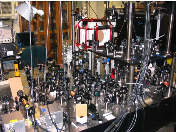
Figure 2: Rubidium cooling and trapping apparatus at Caltech.

[image:10.612.147.430.249.461.2]

(11)

dropping the atoms about a millimeter or two, which would increase our ability to load the traps, but would greatly restrict the number of atoms we could capture in the MOT cloud. I subsequently determined that we could load more atoms by inverting the chip and tossing the atoms up at it from a free-space MOT. The ability to capture up to 1,000 times more atoms in the initial MOT (∼109_{rather than}_∼₁₀6_{) more than compensated for the reduction in loading efficiency by a factor}

of roughly 100. I simulated the launching of classical particles from a Gaussian MOT distribution and found that we could load different levels within the chip trap by changing the time at which we turned on the conservative trapping potential. Inverting the chip also made it easier to imagine how we would detect the trapped atoms: when the DC potential is removed, the atoms will fall away from the surface, where they can be imaged by fluorescence.

A significant downside of the inverted operation is that atoms would travel quite far (several inches) from the trapping MOT to the chip, and therefore needed to be very cold to maintain density. This required sub-Doppler cooling as a part of the atom-tossing procedure. After several months of system optimization (which made the whole apparatus more robust), I was finally able to cool the atoms to below their Doppler temperature one day in the spring of 2007. The next day, however, the magnetic field was distinctly different, and sub-Doppler cooling no longer worked. After scouring the lab for what had changed, I stepped next door into the Eisenstein lab, where I learned that their 13 Tesla superconducting magnet was at a different set-point that day than the day before: culprit identified. I was able to cobble together a sensor above the MOT to measure the background field from their magnet, but stopped work on optimizing that sensor when Hideo announced the lab move to Stanford. My apparatus, built used shared grant money with Prof. Oskar Painter, would stay at Caltech with me, but move to the Painter lab.

As my lab-mates prepared to move to Stanford, I disassembled and packed up my apparatus for the move across campus. I was initially supposed to reassemble in one lab, but there was not enough space. Then I designed the conversion of an office to a lab space, but that was not completed because Prof. Painter won space in a different building, for which he had to give up the space where I was planning to work. While this uncertainty plagued my progress, I continued the design process for an alternative experiment which would have a greater chance of success than the magnetoelectrostatic traps (where the trap loading issue was still going to be very challenging to resolve): plasmonic diffraction gratings for atoms. Standing surface electromagnetic waves, at very short wavelengths due to their confinement in the surface, would allow atoms to be diffracted to large angles. However, as it became clear that I was not going to be able to reassemble my apparatus in time to get results and graduate in a reasonable time, I approached Hideo about a theoretical project, and this thesis project was born. The apparatus I designed and built has been reassembled in the Painter group’s new space, but has not yet been fully integrated into their research.

(12)

(13)

Chapter 1

Introduction and Background

Quantum mechanics forms the basis for our understanding of the behavior of light and matter. While most day-to-day events we observe can be accurately modeled using classical mechanics and electromagnetism, many physical systems require a quantum mechanical description. Whether we are interested in the details of a chemical reaction or the flow of electrons through a semiconductor inside a computer, or even a system as apparently simple as the interaction of the electromagnetic field with a single atom, quantum mechanical modeling is both highly accurate and necessary. As optical networks and computing resources shrink and become faster, they will inevitably encounter limits set by quantum mechanics. While these limits might impose restrictions on the behavior of a system, they may also open the door to other uses for the same system. This thesis is dedicated to examining ways of building simpler models for quantum systems which respect their dynamics, but may eventually also allow those systems to be more easily developed into useful technology.

Quantum mechanics is an inherently probabilistic model for the physical world. In order to model the dynamics of quantum systems, we propagate not a single position and momentum as we might for a classical system, but instead a probability distribution. Undergraduate quantum mechanics usually introduces the Schr¨odinger equation, a partial differential equation for the wavefunction of an isolated physical system, from which we can calculate the possible results of measurements of certain observable quantities. However, as we work to match this simple model with the physical world, we encounter limits to the model. First, we are forced to reckon with the difficulty of building an isolated system, and then measuring it. By definition, the measurement process is an intrusion from the “outside” into a supposedly isolated system. This is usually dealt with by hand-waving arguments about an omnipotent experimenter suddenly introducing a measurement apparatus and making a sharp, projective measurement.

(14)

so that we may retrieve information about the system without disrupting it in ways we do not want. (If we can do this, then we are justified in our model’s separation between “system” and “environment.”) A physical measurement process can almost always be modeled not as a direct measurement of the system, but instead a measurement of the environment interacting with the system of interest. Measurements also necessarily take time; the instantaneous measurement of introductory quantum mechanics is as much an approximation as its isolation.

We must also deal with the fact that our measurement may not tell us everything about our system, because of the limited way in which the environment interacts with the system, or because our measurement cannot distinguish between different states of the environment or, as a result, the system. As experimenters, our understanding of the state of our quantum system is shaped by the system’s history and dynamics (the realm of the Schr¨odinger equation), and also by the fallible way we measure the system, noise which may be introduced through the environment or measurement, or our simple failure to measure all of the parts of the environment which carry information about the system. We must almost always think of our quantum system as being in a mixed state, acknowledging our lack of knowledge about the system.

Mixed states cannot be modeled as wavevectors (|ψi), and must instead be modeled using density matrices (P

ici|ψiihψi|), which we propagate in time using the master equation. Density matrices

reside in a much larger space than wavefunctions — they have many more degrees of freedom — which makes accurate simulations of dynamics a challenge for large systems. In particular, any system which is coupled with an electromagnetic field can be difficult to simulate because the field, modeled as a harmonic oscillator, is infinite dimensional (there’s no top to the ladder of states). It is usually reasonable to define a cut-off energy, but this can still result in very large density matrices, especially if the system consists of tensor products of this large field space with other system components. Coupling with a two-level system quadruples the number of elements in the density matrix.

One way to tackle this challenge is by simulating only fully observed systems. That is, only sys-tems in which the experimenter measures every output channel. Such syssys-tems can be simulated using a stochastic Schr¨odinger equation, and their states remain pure, and take the form of wavefunctions. The quantum simulations (“trajectories”) in this thesis are all of this form. The statistical behavior of such systems is identical to partially observed systems over long times (or multiple samples of identical systems). Measurements should not be able to change the fundamental statistics of the underlying system.

(15)

state of the system, with filter input from the output of the measurement process. The experimenter’s best guess is a mixed state, and propagating the master equation will be computationally intense (and very difficult to do in real time). Should the experimenter desire to use this filter to decide on a control signal to drive the system to a particular state, she will be hard pressed to update her best guess in real time, and the control task will be very challenging. This thesis attempts to develop techniques to build simple models for quantum systems which capture the dynamics of interest (and potential utility) and which may also be propagated much more easily, potentially in real time, by a computer or purpose-built circuit. Such simple models might also provide insight into the system by elucidating the components which result in particular behavior.

The general technique I use to build simpler models is to find a linear or nonlinear submanifold of the full space of possible dynamics, in which the particular dynamics of a system are generally confined. I adapt various techniques for finding such subspaces developed for other applications to the case of quantum dynamics, and illustrate both their successes and failures.

1.1 Thesis overview

The remainder of this Introduction introduces the example physical system whose dynamics we will attempt to model with simple dynamical systems: a two-level atom in a high-finesse optical cavity, a situation known as “cavity quantum electrodynamics” (cavity QED). I review the dominant model for cavity QED, the Jaynes-Cummings model, give an abbreviated derivation of the Maxwell-Bloch equations, and a short summary of known interesting dynamics observed in these equations and in corresponding simulations of cavity QED. I close with a brief introduction to a few topics in stochastic calculus, to lay the groundwork for the remainder of the thesis.

Chapter 2 provides an overview of the technique of projecting filtering equations onto manifolds. I then turn to a particular manifold — a linear space of density matrices — and project the stochastic master equation for cavity QED onto this space, deriving nonlinear dynamical equations for the local coordinates.

Chapter 3 makes the work of Chapter 2 more concrete by describing a process, Proper Orthogonal Decomposition, for determining a linear density matrix space onto which to project the dynamics. I analyze cavity QED dynamics in phase and absorptive bistability regimes, and demonstrate some successes, and some failures, of this process for generating accurate filters.

(16)

absorptive bistability case is more complex, but I lay the groundwork for deriving similar systems of equations.

The concluding Chapter 5 draws the results together, examines the successes and failures of the examined model reduction techniques, and suggests directions for future work.

1.2 Model system: Cavity quantum electrodynamics

A single atom in a high-finesse optical cavity constitutes a canonical system in quantum optics. Experimental work on such systems (such as [3, 4, 5, 6, 7], among many others) has demonstrated strong coupling between the atom and the optical field, meaning that the presence or absence of a single photon drastically changes the environment for a single atom, and correspondingly, that the state of the single atom strongly affects the behavior of the field in the cavity. There are multiple parameter ranges in which strong coupling occurs. Strong coupling can be identified as a regime in which the ratio of the square of the atom-field coupling rate to the product of the cavity decay and atomic spontaneous emission rates is large. This ratio is called the “cooperativity.” Two limits of interest are the “bad cavity” and “good cavity” limits: for a fixed value of the cooperativity, the cavity decay rate may be large compared with the spontaneous emission (“bad cavity”), or small (“good cavity”). We usually scale time by the atomic spontaneous emission rate, so it ends up dropping out; this means that a small cavity decay rate, for a fixed cooperativity, implies a small atom-field coupling rate (inside a higher-finesse cavity), andvice versa.

1.2.1 The Jaynes-Cummings model

A simple model for the atom-cavity system is the Jaynes-Cummings model [8]. In this model, the atom is approximated as a two-level system, there is only one harmonic mode of the field in the cavity. The two-level atom is equivalent to a single spin, and the operators which act on it are the Pauli matrices and their linear combinations: σ− lowers the atom into its ground state, while

σ+=σ†−excites the atom. The field is acted upon byaanda†, the familiar annihilation and creation operators for a simple harmonic oscillator. We operate in a rotating frame, at the frequency of the driving field. The Hamiltonian in this model takes the form

H = ∆ca†a+ ∆aσ+σ−+ig0

¡

a†_σ

−−aσ+

¢

+iE¡

a†₋_a¢

, (1.1)

where ∆c is the detuning between the field and the cavity, ∆ais the detuning between the field and

the atomic transition, g0 is the coupling rate between the atom and the cavity field, and E is the

(17)

• ∆ca†a accounts for the difference in energy between on- and off-resonant drive of the cavity

by the external field.

• ∆aσ+σ− similarly accounts for the difference in energy between on- and off-resonant drive of the atom by the external field.

• ig0¡a†σ−−aσ+¢is responsible for exchange of energy between the atom and the field at rate

2g0. The first term creates an excitation in the field, while driving the atom to the ground

state; that is, the atom emits a photon into the field. The second is the inverse process, where the atom absorbs one photon out of the field, and becomes excited.

• iE¡

a†₋_a¢

is the external driving field, acting to excite the phase quadrature of the cavity mode.

A Hamiltonian like (1.1) would suffice if we were concerned only with the unobserved dynamics of a closed quantum system. However, for useful systems, the “closed” model will not suffice. Instead, we must extend the picture to include the system’s interaction with its environment, and the behavior of an observer making measurements on the system. The observer may know the quantum state fully, or imperfectly, and so we model the dynamics of such an “open quantum system” with a master equation, which propagates the motion of a density matrix. The interaction of the system and its environment is governed by probabilities, so that the time at which the atom or field changes state (such as emitting a photon) is random. We therefore require a stochastic model for the propagation of the density matrix, which allows for the introduction of noise resulting from this inherently probabilistic behavior.

The Itˆo form of the stochastic master equation (SME) which governs the behavior of an atom-cavity system being observed with homodyne measurements of both the leaking atom-cavity field and the atomic emission is

dρ = −i[H, ρ]dt+κ¡

2aρa†₋_a†_aρ₋_ρa†_a¢

dt

+γ(2σ−ρσ+−σ+σ−ρ−ρσ+σ−)dt

+i√2κ¡

ρa†−aρ−Tr[ρ¡

a†−a¢

]ρ¢

dW1

+ip

2γ(ρσ+−σ−ρ−iTr[ρ(σ+−σ−)]ρ)dW2. (1.2)

Here dW1 and dW2 are uncorrelated Wiener processes corresponding to noise on the two different

(18)

a Fabry-Perot cavity of the sort we model does not significantly change the spontaneous emission characteristics of the atom. The cooperativity parameter mentioned above is defined asC= g

2 0

2κγ⊥ =

g2

0

κγ.

This stochastic master equation will maintain the purity of an initial state, because all the channels of information leaving the system are being measured. As a result, this equation is exactly equivalent to a stochastic Schr¨odinger equation (SSE), which is relatively easy to simulate due to its more benign linear scaling behavior with the number of field modes to be propagated. I will refer to the pure states which result from the propagation of such an equation asquantum trajectories, and they will be a prime source of our insight into system behavior from simulations throughout this thesis. My discussion of quantum trajectories here is grounded in the work of Mabuchi and Wiseman [9] and references therein, although for convenience I have created a somewhat narrower definition of quantum trajectories as pure state trajectories only. I calculate these trajectories throughout the thesis using the SSE integration built in to the Quantum Optics Toolbox for Matlab, written by Sze Tan [10].

The experimentalist is generally unable to measure the field leaking out the sides of the cavity, and has only the measurement record from the cavity field measurement. As a result, she must average over all possible measurement results for the missing atomic measurement, leaving a (likely) mixed state as her best state of knowledge about the system. The density matrix in this case evolves according to the following SME:

dρ = −i[H, ρ]dt+κ¡

dt

+γ(2σ−ρσ+−σ+σ−ρ−ρσ+σ−)dt

+i√2κ¡

ρa†₋_aρ₋_Tr[_ρ¡

a†₋_a¢

]ρ¢

dW. (1.3)

It is this equation which we will project onto low-dimensional subspaces to produce reduced-order models (which we will then use as simple filters), and we will also use it to derive stochastic equations of motion for expectation values of system operators.

1.2.2 Filtering

(19)

represents the new information which the experimenter receives through her measurement, and is called theinnovation. The innovation is defined as the difference between the measurement result and what the observer expected the result to be. In the case of a homodyne measurement of the phase quadrature of the cavity field, for example, the innovation ismeasurement−expectation=

dY − i

2

a†₋_a®

. That this is a Wiener process reflects that the innovation is unbiased — the experimenter learns as much from a measurement result that is larger than her expectation as from a result that is smaller [11].

1.3 The Maxwell-Bloch equations

In my efforts to derive simple classical (or semi-classical) models to approximate quantum systems, the canonical relevant example of such a simplification serves as a constant point of comparison. The Maxwell-Bloch equations are a set of five, coupled, deterministic differential equations for the expectation values of the five simplest operators in this system: a, a†_, _σ_−, _σ

+, and σz. The first

four will be familiar from the Hamiltonian; the last, σz, corresponds to the population difference

between the atomic excited and ground states, and allows the system of equations to close without stretching any approximations to the breaking point. These operators may be combined to create the Hermitian operators

x = 1

2

¡

a+a†¢

y = i

2

¡

a†₋_a¢

σx = σ++σ−

σy = i(σ−−σ+). (1.4)

These Hermitian operators correspond to possible observables of the atom-cavity system. xis the cavity field’s amplitude quadrature; y is its phase. Using the spin analogy with a two-level atom, the Pauli matrixσxis the atomic component along thexaxis, and similarly forσy andσz.

(20)

we derive this set of equations:

dhai = −κ(1 +iΘ)haidt+g0hσ−idt+Edt+i

√ 2κ¡

a(a†−a)®

−

a†−a®

hai¢

dW

d

a†®

= −κ(1−iΘ)

a†®

dt+g0hσ+idt+Edt+i

√ 2κ¡

a†₍_a†₋_a₎®

−

a†₋_a®

a†®¢

dW

dhσ−i = −γ(1 +i∆)hσ−idt+g0haσzidt+i

√ 2κ¡

σ−(a†−a)®

−

a†−a®

hσ−i¢

dW

dhσ+i = −γ(1−i∆)hσ+idt+g0

σza†

®

dt+i√2κ¡

σ+(a†−a)

®

−

a†₋_a®

hσ+i

¢

dW

dhσzi = −2γ(1 +hσzi)dt−2g0a†σ−+σ+a®dt

+i√2κ¡

σz(a†−a)®−a†−a®hσzi¢dW. (1.5)

This system of equations, however, is not closed: it includes the expectation values of products of operators. If we make thead hocapproximation that these operator products can simply be factored (hABi → hAi hBi), we are effectively neglecting correlations between observables (especially the correlations between the atom and the field), of the sort we might expect to see in quantum-limited behavior. However, this dramatically simplifies the system of equations. In particular, it eliminates all of the stochastic terms:

dhai = −κ(1 +iΘ)haidt+g0hσ−idt+Edt

d

a†®

= −κ(1−iΘ)

a†®

dt+g0hσ+idt+Edt

dhσ−i = −γ(1 +i∆)hσ−idt+g0hai hσzidt

dhσ+i = −γ(1−i∆)hσ+idt+g0hσzi

a†®

dt

dhσzi = −2γ(1 +hσzi)dt−2g0¡a†®hσ−i+hσ+i hai¢dt. (1.6)

This resulting set of equations is known as the Maxwell-Bloch equations, and has its origins in a separate, semi-classical derivation [12]. The Maxwell-Bloch equations are derived by extending the optical Bloch equations (which characterize the excitation and coherence of a two-level atomic medium) to include interaction with a resonant (or near-resonant) coherent optical field, for example in a laser.

(21)

1.4 Bistability and other interesting dynamics

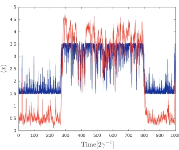
The quantum dynamical system defined by the master equations (1.2) and (1.3) is known to exhibit several interesting behaviors, some of which correspond with the behavior of the Maxwell-Bloch equations (1.6). Of particular interest for this thesis are two parameter regimes in which the dynamics of both quantum and classical systems are “bistable.” In classical, deterministic dynamics, a bistable system is one with two stable (or asymptotically stable) equilibria, and the system settles towards one or the other depending on initial conditions [13]. For the stochastic and quantum cases in this research, I have adapted this term, and assigned it a more phenomenological definition: a system is bistable if its dynamics show it to have two zones of phase space in which it is relatively stable. Noise may drive the system from one stable zone to the other (and back). I will commonly refer to the two zones as states, although they may not correspond to individual quantum states. The zones may roughly correspond to the stable points of a bistable deterministic system, or they may not. A more rigorous definition is likely possible using the techniques and language developed in stochastic dynamical systems theory (for background and foundations, see [14], [15] and [16]), but I have chosen this phenomenological definition for simplicity.

Bistability is useful in the engineering of practical devices, in particular for switching and binary memory. It is intimately related to hysteresis, in which a system prepared through two (or more) different time-varying processes settles into different stable states for the same set of system pa-rameters. Static memory for computing makes use of the bistable behavior of magnetic domains — prepared with strong fields in one direction, they hold that state until actively switched. Most useful bistable systems are relatively noise-free, which contributes to their utility. As performance demands increase, however, devices must become smaller and faster, pushing them into the limit where their behavior is affected by thermal noise, and potentially quantum fluctuations. Current engineered devices are many orders of magnitude more energetic than the relevant quantum limits, but novel technologies for communication and computing (such as those developed for quantum computation and key distribution) may eventually approach it. Stabilizing the two “stable” states of a quantum bistable system in real time would require a model of the underlying quantum dynamics which can be computed alongside the system itself. This thesis is, in part, an attempt to examine potential tools which can be used to make such models, and evaluate their accuracy and utility.

(22)

0 2

4 6

8 -4

-2 0 2 4 0 0.05 0.10 0.15

(a)

-2 0

2 4

6 8 -5

0 5

0 0.02 0.04 0.06 0.08 0.1

[image:22.612.92.493.83.233.2]

(b)

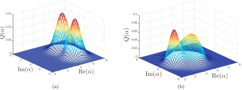
Figure 1.1: Q functions for the field modes of two bistable Cavity QED parameter regimes. (a) Phase bistability. (b) Absorptive Bistability.

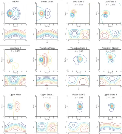
zone) is much broader than a minimum-uncertainty state, and has significant variation in its phase. The appearance of the system from the observer’s standpoint, then, is a system whose absorption changes suddenly between two values, thus “absorptive bistability.” The relative ease of measuring field amplitude makes absorptive bistability particularly inviting for use as an optical switch or bit of memory. For both types of bistability, if one does a partial trace over the atomic portion of the density matrix, the Q function of the resulting field state takes the form of a bimodal distribution (Figure 1.1).

Phase bistability has been the subject of numerous publications over the course of the past twenty years. First noted by Alsing and Carmichael [17] and Kilin and Krinitskaya [18], it was further investigated by Mabuchi and Wiseman [9], who simulated the noisy switching behavior in a quantum trajectory formulation using the full stochastic master equation with homodyne detection to measure the phase quadrature directly, and no measurement of the spontaneous emission (following the example of Carmichael and collaborators [19], who modeled the system with homodyne detection of the cavity field and direct photo-detection of the atomic decay). Phase bistability occurs for resonant conditions (driving field, cavity, and atom all resonant), with a large driving fieldE relative to the atom-cavity couplingg0, andg0 large compared to the atomic spontaneous emission rate. In

the limit of no atomic spontaneous emission (γ= 0), the Maxwell-Bloch equations have two stable points [17]

hai± =

E+g0hσ−i±

κ

hσ−i± = −g0

4E ∓i

·₁

4 −

³g₀

4E

´2¸1/2

hσzi = 0, (1.7)

(23)

that forE ≫g0, the two stable points become orthogonal quantum states. They now correspond to

two coherent states of the field, each paired with an atomic state in a superposition of the excited and ground states, but with opposite phases. When we let γ 6= 0, but still small, the resulting spontaneous emission events correspond to the system switching between the two stable states [19]. Van Handel and Mabuchi [11] examined the phase bistable state from the perspective of pro-jection filtering. They defined a three-dimensional, nonlinear manifold: one dimension measures the relative populations of two gaussian field states (paired with the corresponding atomic state appropriate for their phase), and the other two dimensions reflect the positions of the two gaussians. After an excellent, clear derivation of the filtering equation and rules for projecting it, they project the master equation onto this nonlinear manifold and derive a nonlinear set of stochastic differential equations to use as a simple filter. This filter behaves almost identically to the optimal filter, despite its simplicity, which implies that the underlying dynamics are fundamentally quite simple. If we take the two gaussian field modes to be fixed, the resulting 1-dimensional system is identical to the filter for a stationary Markovian jump process (the Wonham filter). Our analysis of the geometry of this system in Chapter 4 focuses on the geometry of the switching behavior; we should expect that the dynamics we derive will require the inclusion of the state position variables to characterize the transitions.

The Maxwell-Bloch equations may be examined as classical dynamical systems in order to search for regimes with interesting behavior which may correspond to novel behavior in the related quantum system. Gang, Ning, and Haken ([20] and [21]; see [21] for a summary of earlier related, but limited, work by others) undertook a search for these regimes, and Armen and Mabuchi [22] extended this search and analyzed the behavior of quantum systems in several regimes. They examined the absorptive bistability regime (which I use as an example system to evaluate model reduction techniques in this thesis), as well as behavior near both super- and sub-critical Hopf bifurcations, which lead to classical systems exhibiting limit cycles surrounding stable or unstable fixed points. Absorptive bistability may be predicted by semi-classical analysis of a saturable absorber in an optical cavity [23]. Savage and Carmichael [24] were the first to examine the single-atom case using the model described here, and discuss how quantum fluctuations would affect the system.

(24)

0 1 2 3 4 5 6 7 8 9 10 11

[image:24.612.158.410.90.305.2]

0.35 0.4 0.45 0.5 0.55 0.6

Figure 1.2: Semiclassical intracavity steady state field magnitude as a function of drive fieldE, from [22]. The dashed portion indicates an unstable equilibrium. The parameter values are: g0 =

√ 2,

γ = 2, κ= 0.1, Θ = 0, and ∆ = 0 (with γ⊥ = 1 setting the scaling of time). The point used to examine absorptive bistability in this thesis hasE = 0.56.

(25)

understand this system.

1.5 An aside on stochastics

I will now give a brief overview of some results from stochastic calculus, to lay the groundwork for their use later in the thesis. These notes skim only the very surface of the field; I recommend Gardiner [25] and van Kampen [26] for more information. In stochastic calculus, we commonly have a Wiener process (usually denoted W), which is a continuous-time stochastic process which can be thought of as the integral of white noise. Rigorously, the differential form of writing stochastic equations of motion is nothing but a shorthand for the integral form. In stochastic differential equations, however, we write a stochastic incrementdW, which is like a stochasticdt. We generally choose to scale it so that the mean value ofdW2 _is_dt_{, or “}_dW _∼√_dt_.”

In classical, deterministic analysis, the integral can be defined as the sum of intervals, and in the limit of infinitesimal intervals, it does not matter whether we have chosen at each interval to use the function value at the start, middle, or end of the interval. In defining the stochastic integral, however, it does matter. We are forced to make a choice regarding which side of the infinitesimal interval to choose when summing, as they produce different results. The most common choices are those made by Itˆo and Stratonovich. Itˆo chose the start of each interval, while Stratonovich chose the midpoint. A given stochastic differential equation, therefore, must be accompanied by information about which kind of SDE it is. I follow the standard practice of writing◦dW for Stratonovich, and simplydW

for Itô. Almost every equation in this thesis is in Itô form. There are many integrators designed for stochastic systems (see [27] for a summary), but I have restricted my work to a simple Itô-Euler integrator. (This is simply an Euler integrator with a stochastic term added.) When numerically integrating an SDE using this method, you must use the Itô form of the equation, because you are implicitly choosing the value at the start of each time interval for your integration. Other integrators use the Stratonovich form, or (like the Milstein integrator) add different correction terms.

Let us assume we have an Itˆo stochastic differential equation

dR(x, t) =A(x, t)dt+B(x, t)dW. (1.8)

In order to transform this to the equivalent Stratonovich SDE, we mustsubtract the “Itˆo correction term”

1

(26)

B .) Similarly, if we have a Stratonovich SDE

dR(x, t) =A(x, t)dt+B(x, t)◦dW, (1.10)

weadd the Itˆo correction term (1.9) to transform it into Itˆo form.

The other critical difference between Itˆo and Stratonovich forms, for the purposes of this thesis, is how they respond to a transformation of coordinates. Projecting equations of motion, as I will do in Chapters 2 and 3, is such a transformation of coordinates. Under a transformation ¯x=φ(x), the coordinates of (1.8) transform into

¯

A(¯x) = A(x)dφ

dx +

1

2(B(x, t))

2d2φ

dx2

¯

B(¯x) = B(x)dφ

dx. (1.11)

In contrast, the coordinates in the Stratonovich form transform like vectors (with no second-order derivatives):

¯

A(¯x) = A(x)dφ

dx

¯

B(¯x) = B(x)dφ

dx. (1.12)

(27)

Chapter 2

Projection Filters

Dynamics of open quantum systems take place in the space of density matrices, which can be a very high dimensional space, particularly when photon fields are involved. Strictly speaking, density matrices including photons are infinite, but it is common in practice to introduce a cutoff at some high Fock state, and work with finite, but large, density matrices. In simulations of cavity QED with the Jaynes-Cummings model, desired accuracy commonly requires one to keep track of 100 or more Fock states, in addition to the two-level atom. This results in a density matrix that is at least 200×200, indicating that the dynamics take place in a space that is nominally 39,999-dimensional (anN×N density matrix hasN2₋_{1 real degrees of freedom, taking Hermiticity into}

account). However, we know that the dynamics of a particular system do not fully explore this space, and as a result we would like to define a smaller (lower-dimensional) space, and study the system dynamics within that space alone. To do this, we project the equations of motion onto the lower-dimensional space. In this chapter I give a short overview of how to calculate these projected equations of motion, put this projection in the context of stochastic filtering equations, and then derive the form of the projected equations for the cavity QED master equation for a particular form of the lower-dimensional space: a linear density matrix space.

2.1 Filter projection in general

In this section, I will give a brief overview of the process of projecting equations of motion from a high-dimensional manifold onto a lower-high-dimensional one. I draw heavily upon the excellent description of this process given by van Handel and Mabuchi [11], adapting their derivation to the case of density matrices (instead of Q functions). Let us denote the space of all possible density matrices for a quantum system of interest by M, and the smaller subspace by S. Let our example stochastic dynamical system take the form

(28)

From a geometric standpoint, we would like to think of the right-hand side of this equation as a vector in the tangent space toM at a particular pointθM. When we project the equation ontoS,

we would like to keep the components which are in the tangent space toS atθ, denotedTθS, and

discard the components in the orthogonal complement to this tangent space, denotedTθS⊥. For the

right-hand side of Eqn. (2.1) to be treated as a vector, it must transform like one, which means we must interpret it as a Stratonovich stochastic differential equation, rather than an Itˆo equation. For now I will simply change the notation to reflect this, but in a practical situation (like that following, in Sec. 2.2), one would calculate the appropriate Itˆo correction term, which would change the forms ofAandB. The new equation takes the form

dρt=A[ρt]dt+B[ρt]◦dWt. (2.2)

If we assume that we have a local coordinate system onSso thatθ= (θ1, θ2, . . .), then we can write

TθS = Span

·

∂ρ(θ)

∂θ1 ,

∂ρ(θ)

∂θ2 ,· · ·

¸

. (2.3)

We define an inner product on the space of density matrices

hρA, ρBi= Tr[ρAρB], (2.4)

which allows us to calculate the metric tensor in this basis:

¿

∂ρ(θ)

∂θi ,

∂ρ(θ)

∂θj

À

= Tr

·

∂ρ(θ)

∂θi

∂ρ(θ)

∂θj

¸

=gij(θ). (2.5)

If the basis defined in Eqn. (2.3) is orthonormal,g will simply be the Identity; otherwise it accounts for the non-orthonormality. With an inner product and a metric, we can define orthogonal projection of a vector fieldX[θ]:

ΠθX[θ] =

X

i

X

j

gij(θ)

¿

X[θ],∂ρ(θ) ∂θj

À

∂ρ(θ)

∂θi , (2.6)

wheregij _{denotes the (}_{i, j}_{) component of the inverse of the metric}_g_{defined in Eqn. (2.5).}

We now wish to constrain the dynamics of Eqn. (2.2) to evolve onS:

dρ(θt) = ΠθtA[ρ(θt)]dt+ ΠθtB[ρ(θt)]◦dWt, (2.7)

which is just a stochastic differential equation for the parameters θt. Next, note that, in the

Stratonovich calculus,

dρ(θt) =

X

i

∂ρ(θt)

∂θi t

◦dθi

(29)

If we insert the definition of the orthogonal projection into Eqn. (2.2), we see that

dρ(θt) =

X

i

X

j

gij(θ)

¿

A[ρ(θt)],∂ρ(θ)

∂θj

À

∂ρ(θ)

∂θi dt

+X

i

X

j

gij(θ)

¿

B[ρ(θt)],

∂ρ(θ)

∂θj

À_∂ρ₍_θ₎

∂θi ◦dWt. (2.9)

Comparing this expression with Eqn. (2.8), we can pull out the equations fordθi t:

dθi

t=

X

j

gij₍_θ₎

¿

A[ρ(θt)],

∂ρ(θ)

∂θj

À

dt+X

j

gij₍_θ₎

¿

B[ρ(θt)],

∂ρ(θ)

∂θj

À

◦dWt. (2.10)

Note that in order to apply this procedure, we need to know a functional form for ρ(θ), meaning we need a map from the smaller space (spanned by θ) to the larger space (where ρlives). This is in addition to knowing the form of the projection from the larger space to the smaller, facilitated by Eqn. (2.6) and the like. (The manifold learning algorithms discussed in Chapter 4 provide only point-wise maps, so projecting the filters onto them will be a challenge.)

When we want to use these projected equations as a filter, the measurement photocurrent driving them is still the same as that which drives the full-space SME (thought of as a filter). The innovation process, dW, however, is different because it is defined as the difference between the measurement result and the filter’s current estimate, which differs for each filter. Assuming that we can construct the map which reverses the projection Π, giving us aθM from eachθ, we can directly compare the

state generated by the projected equations of motion (2.10) with the corresponding trajectory. We should be careful to note that the projected equations will often be generated from an SME which does not correspond to measuring every output from the system, whereas a quantum trajectory simulation necessarily requires measurement of all outputs so as to allow the creation of a stochastic Schr¨odinger equation. In order to reduce the difference between these two cases for cavity QED, in trajectory simulations I have consciously chosen to measure the atomic spontaneous emission in the quadrature which gives the least additional information about the system in its measurement record (for both absorptive and phase bistability, this is theσy quadrature). It is possible that differences

persist, but they ought to be minor because the trajectories are required to average (over long times or many runs) to the same mean as for the unmeasured-atom situation reflected in Eqn. (1.3).

2.2 Projecting onto a linear density matrix space

2.2.1 The stochastic master equation

(30)

field leaking out of the cavity. This is the normalized Itˆo form of the equation, for homodyne measurement of the phase quadrature:

D[ρ] = −i[H, ρ]dt+κ¡

2aρa†−a†aρ−ρa†a¢

dt

+γ¡

2σρσ†₋_σ†_σρ₋_ρσ†_σ¢

dt

+√2κ¡

ρa†₋_aρ₋_i_Tr[_ρ¡

a†₋_a¢

]ρ¢

dW. (2.11)

If we wanted to measure the amplitude quadrature instead, we would replaceawithiaeverywhere outside of the Hamilitonian. If we removed the nonlinear term Tr[ρ¡

a†₋_a¢

]ρ, we would have the un-normalized version of the SME. It has the distinct advantage of being linear, but will allow the trace of the density matrix to differ from 1. In a stochastic simulation, we can use the unnormalized equation, and simply renormalize ρafter each time step. However, for completeness, and because the filters from the normalized equation seem to be better “behaved,” I chose to use the normalized form, with its attendant complications resulting from nonlinearity.

In order for the geometry of projection to make sense, we need the components in this equation to transform like vectors, which means it needs to be a Stratonovich equation. We have two options for undertaking this transformation: 1) calculate the Itˆo correction term for Eqn. (2.11) or 2) use the much simpler (linear) un-normalized equation, transform it to Stratonovich form, and then normalize. I choose to do the first. This is the correct normalized Stratonovich form of the equation, calculated directly from Eqn. (2.11), for homodyne measurement of the phase quadrature:

D[ρ] = −i[H, ρ]dt+κ¡

dt

+γ¡

2σρσ†−σ†σρ−ρσ†σ¢

dt

−κ³2aρa†−a2ρ−ρ¡

a†¢2

+ 2Tr[(a†−a)ρ](ρa†−aρ)

−2ρ¡

Tr[(a†−a)ρ]¢2

+ρ£

Tr[(a†−a)(ρa†−aρ]¤´

dt

+i√2κ¡

a†₋_a¢

]ρ¢

◦dW, (2.12)

where the HamiltonianH is as in Eqn. (1.1), anddW is the innovation.

2.2.2 The density matrix

(31)

detailed form of such a space and the mechanics of the projection.

Imagine an N-dimensional linear density matrix space. Density matrices in this space have the following form:

ρ(v) =ρ0+

N

X

i=1

viρi (2.13)

where theρis are trace-0 Hermitian matrices (directions in density-matrix space), andρ0is a positive,

trace-1 Hermitian matrix (a valid density matrix), which serves as the origin in our linear space. The coefficients vi are real, to maintain Hermiticity. There is nothing that forces ρ(v) to remain

positive, so it might cease to be a valid density matrix. However, when acting as part of a filter we expect it to stay positive almost all the time, except when presented with a measurement record which it is unable to do a good job of accommodating.

The partial derivatives of ρare

∂ρ(v)

∂vi =ρi. (2.14)

We recall the definition of the inner product between matrices/operators as the trace of the product, and so we define the metric in this space

gij = Tr[ρiρj] (i, j >0). (2.15)

We assume that theρis have been orthonormalized so thatgij =gij =δij (g= Id).

If we had not used the normalized form of the stochastic master equation, we would have extended the dimension of the linear space by 1 to include a coefficient onρ0. Then we would redefine the

state to be the ratio of each coefficient tov0, which would complicate the equations to be evolved.

Alternatively, in simulations, we would simply rescale all of the coefficients at each time step, setting

vi = ˜vi/v˜0, i≥0. In practice, filtering using the normalized equations seems to be somewhat more

robust, and it has the advantage of providing us with exact, nonlinear equations directly.

2.2.3 Projection

Following the general derivation given in Section 2.1, and specializing to our particular space S, spanned by the statesρi, we have that the orthogonal projection of (2.12) is

ΠvD[ρ(v)] = N

X

i=1

N

X

j=1

gij

¿

D[ρ(v)],∂ρ(v) ∂vj

À_∂ρ₍_v₎

∂vi . (2.16)

Simplifying because we know thatgij=gij=δij, we see that

ΠvD[ρ(v)] = N

X

i=1

(32)

For an arbitrary filtering SME of the form (2.2), we constrain the filter to evolve in our space of density matrices, and combine Eqn. (2.17) with Eqn. (2.7) to find that

dvi=hA[ρ(v)], ρiidt+hB[ρ(v)], ρii ◦dW. (2.18)

We have split the master equation, Eqn. (2.12), into deterministic and stochastic parts, as in Eqn. (2.2), to clarify calculation:

A[ρ] = −i[H, ρ] +κ¡

+γ¡

2σρσ†−σ†σρ−ρσ†σ¢

−κ³2aρa†₋_a2_ρ

−ρ¡

a†¢2

+ 2Tr[(a†₋_a₎_ρ_](_ρa†₋_aρ₎

−2ρ¡

Tr[(a†₋_a₎_ρ_]¢2

+ρ£

Tr[(a†₋_a₎₍_ρa†₋_aρ_)]¤´

(2.19)

B[ρ] = i√2κ¡

a†₋_a¢

]ρ¢

. (2.20)

We will now project each of these terms, in order to derive the detailed form of Eqn. (2.18).

2.2.4 The deterministic terms A[

ρ

]

Let us start calculating the terms in (2.18). First, we define

LH(ρ) ≡ −i[H, ρ] (2.21)

La(ρ) ≡ κ¡2aρa†−a†aρ−ρa†a¢ (2.22)

Lσ(ρ) ≡ γ¡2σρσ†−σ†σρ−ρσ†σ¢ (2.23)

LISL(ρ) ≡ κ

³

2aρa†−a2ρ−ρ¡

a†¢2´

(2.24) LISN(ρ) ≡ κ

³

2Tr[(a†₋_a₎_ρ_](_ρa†₋_aρ₎₋₂_ρ¡

Tr[(a†₋_a₎_ρ_]¢2

+ρ£

Tr[(a†₋_a₎₍_ρa†₋_aρ_)]¤´

. (2.25)

Then

hA[ρ(v)], ρii = hLH(ρ(v)) +La(ρ(v)) +Lσ(ρ(v))

−LISL(ρ(v))− LISN(ρ(v)), ρii (2.26)

= hLH(ρ(v)), ρii+hLa(ρ(v)), ρii+hLσ(ρ(v)), ρii

(33)

Expanding the form ofρ(v), we have

hLH(ρ(v)), ρii =

*

LH(ρ0+

N

X

j=1

vjρj), ρi

+

(2.28)

= hLH(ρ0), ρii+ N

X

j=1

vjhLH(ρj), ρii, (2.29)

and the same forLa,Lσ, andLISL, because they are all linear inρ.

In fact, if we define

L ≡ LH+La+Lσ− LISL (2.30)

then we have

hL(ρ(v)), ρii=hL(ρ0), ρii+ N

X

j=1

vjhL(ρj), ρii. (2.31)

Plugging this into Eqn. (2.18), we see that the linear, deterministic part ofdvis

dvi(lindet)=hL(ρ0), ρii+

N

X

j=1

vjhL(ρj), ρiidt. (2.32)

If we think of dv as a vector, we see that this is just a matrix multiplication, where each entry in the matrixLis simply

Lij=hL(ρj), ρii+hL(ρ0), ρiiδij. (2.33)

Now we need to take a look atLISN, the nonlinear terms from the Itˆo to Stratonovich conversion.

LISN(ρ) ≡ κ

³

2Tr[(a†₋_a₎_ρ_](_ρa†₋_aρ₎₋₂_ρ¡

Tr[(a†₋_a₎_ρ_]¢2

+ρ£

Tr[(a†₋_a₎₍_ρa†₋_aρ_)]¤´

. (2.34)

Let us start with the first term, and plug in the approximate form ofρfor our linear space.

Tr



(a†−a) 

ρ0+

N

X

j=1

vjρj

      

ρ0+

N

X

j=1

vjρj



a†−a 

ρ0+

N

X

j=1

vjρj



 



= Tr[(a†−a)ρ0](ρ0a†−aρ0) + Tr[(a†−a) (ρ0) ]

    N X j=1

vjρj



a†−a 



N

X

j=1

vjρj

    +Tr 

(a†−a) 



N

X

j=1

vjρj



 

((ρ0)a†−a(ρ0))

+Tr



(a†−a) 



N

X

j=1

vjρj

        N X j=1

vjρj



a†−a 



N

X

j=1

vjρj



 

(34)

= Tr[(a†−a)ρ0](ρ0a†−aρ0) + Tr[(a†−a)ρ0]

X

k=1

vk(ρka†−aρk)

+

N

X

j=1

vjTr[(a†−a)ρj](ρ0a†−aρ0) +

N

X

j=1

vjTr[(a†−a)ρj] N

X

k=1

vk(aρk+ρka†)

=



Tr[(a†−a)ρ0] +

N

X

j=1

vjTr[(a†−a)ρj]



× Ã

(ρ0a†−aρ0) +

N

X

k=1

vk(ρka†−aρk)

!

.(2.35)

Now, let us do the inner product with ρi, noting that the traces are things we have calculated

anyway, because they’re just the expectation values of−2iy for eachρj:



Tr[(a†−a)ρ0] +

N

X

j=1

vjTr[(a†−a)ρj]





×

*

(ρ0a†−aρ0) +

N

X

k=1

vk(ρka†−aρk), ρi

+

= −2i



hy0i+

N

X

j=1

vjhyji



× Ã

(ρ0a†−aρ0), ρi

® + N X k=1 vk

(ρka†−aρk), ρi

® !

.

(2.36)

It doesn’t simplify much because we can’t use the orthogonality of the ρis once the as are present.

For simulations, however, we can pre-calculate the values of everything in the angle brackets.

Let us take the third term, the other quadratic term:



ρ0+

N

X

j=1

vjρj



Tr 

(a†−a) 

 

ρ0+

N

X

j=1

vjρj



a†−a 

ρ0+

N

X

j=1

vjρj

     

= ρ0Tr[(a†−a)(ρ0a†−aρ0)] +ρ0

N

X

k=1

vk£Tr[(a†−a)(ρka†−aρk)]¤

+

N

X

j=1

vjρj£Tr[(a†−a)(ρ0a†−aρ0)]¤

+

N

X

j=1

vjρj N

X

k=1

=

Ã

Tr[(a†₋_a₎₍_ρ

0a†−aρ0)] +

N

X

k=1

!

×



ρ0+

N

X

j=1

vjρj



(35)

This does simplify once we do the inner product withρi:

hρ0, ρii+ N

X

j=1

vjhρj, ρii=Gi+vi (2.38)

where

Gi ≡ hρ0, ρii. (2.39)

And now for the cubic term:



ρ0+

N

X

j=1

vjρj



 Ã

Tr

"

(a†₋_a₎

Ã

ρ0+

N

X

k=1

vkρk

!#!2

. (2.40)

Noting the above simplification, we see that after we do the inner product, we have this:

(Gi+vi)

³

Tr£

(a†₋_a₎_ρ

0¤ 2 + 2 N X k=1

vkTr£(a†−a)ρ0¤Tr£(a†−a)ρk¤

+ N X j=1 N X k=1

vjvkTr£(a†−a)ρj¤Tr£(a†−a)ρk¤

´

= −4 (Gi+vi)

³

hy0i2+ 2

N

X

k=1

vkhy0i hyki+ N X j=1 N X k=1

vjvkhyji hyki

´

. (2.41)

Assembling all of the parts ofLISN(ρ) together, we have:

dvi(ISN) = − hLISN(ρ), ρiidt

= −κ

Ã

−4i



hy0i+

N

X

j=1

vjhyji



× Ã

(ρ0a†−aρ0), ρi®+ N

X

k=1

vk(ρka†−aρk), ρi®

!

+8 (Gi+vi)

Ã

hy0i+

N

X

k=1

vkhyki

!2

+(Gi+vi)

Ã

Tr[(a†−a)(ρ0a†−aρ0)] +

N

X

k=1

! !

dt.

(2.42)

2.2.5 The stochastic terms B[

ρ

]

Recall that

B[ρ] =i√2κ¡

a†₋_a¢

]ρ¢

(36)

The linear portion of this [LS(ρ)≡i 2κ ρa −aρ ] is just like the deterministic case, with

dvi(lin)=hLS(ρ0), ρii+ N

X

j=1

vjhLS(ρj), ρii ◦dW, (2.44)

and will work out to a simple, constant over time, matrix multiplication by a matrixLS:

LSij =i

√ 2κ¡

ρja†−aρj, ρi®+ρ0a†−aρ0, ρi®δij¢, (2.45)

Now let us turn to the nonlinear term:

i

Tr[ρ(v)¡

a†₋_a¢

]ρ(v), ρi

® =i * Tr   

ρ0+

N

X

j=1

vjρj



 ¡

a†₋_a¢ 

 Ã

ρ0+

N

X

k=1

vkρk

!

, ρi

+

. (2.46)

This breaks out into 4 chunks: A constant (independent ofvi),

i

Tr[ρ0¡a†−a¢]ρ0, ρi®, (2.47)

two linear terms:

i

*

Tr[ρ0¡a†−a¢]

Ã N

X

k=1

vkρk

!

, ρi

+ and (2.48) i * Tr     N X j=1

vjρj



 ¡

a†−a¢ 

ρ0, ρi

+

, (2.49)

and one quadratic term:

i * Tr     N X j=1

vjρj



 ¡

a†−a¢ 

 ÃN

X

k=1

vkρk

!

, ρi

+

. (2.50)

Many of the components of these terms are constants.

The constant term is

2Gihy0i, (2.51)

and the two linear terms are

2hy0i

N

X

k=1

vkhρk, ρii= 2hy0i

N

X

k=1

vkδik= 2hy0ivi (2.52)

and

2Gi N

X

j=1

(37)

The quadratic term is 2 N X j=1 N X k=1

vkvjhyji hρk, ρii= 2 N X j=1 N X k=1

vkvjhyjiδki= 2vi N

X

j=1

vjhyji. (2.54)

The stochastic part of Eqn. (2.18) from the nonlinear (trace) term is therefore

dvi(trace) = −

√ 8κ



hy0iGi+hy0ivi+Gi N

X

j=1

vjhyji+vi N

X

j=1

vjhyji



◦dW

= −√8κ



hy0iGi+hy0ivi+ (Gi+vi) N

X

j=1

vjhyji



◦dW. (2.55)

So, putting all of Eqn. (2.18) together we have

dvi =



hL(ρ0), ρii+ N

X

j=1

vjhL(ρj), ρii



dt+dvi(ISN)

+



hLS(ρ0), ρii+ N

X

j=1

vjhLS(ρj), ρii



◦dW

−√8κ(Gi+vi)



hy0i+

N

X

j=1

vjhyji



◦dW. (2.56)

2.2.6 Stratonovich back to Itˆ

o

For numeric simulation with an Itô-Euler integrator, we require Itô equations, so we need to trans-form our Stratonovich equations back into Itô. Currently our equations of motion for the projected filter have the form

D[v] =Av[v]dt+Bv[v]◦dW. (2.57)

The correction term has the form

1

2(DBv[v])Bv[v] (2.58) whereD(·) is the derivative.

TheLS part of the stochastic term is just matrix multiplication byLS, so its derivative is just

(38)

The part of B that comes from the normalizing term in the SME has a derivative of

DBv(trace)[v]ij = − ∂

∂vj

√ 8κ

Ã

hy0iGi+hy0ivi+ (Gi+vi) N

X

k=1

vkhyki

!

= −√8κ

Ã

hy0iδij+ (Gi+vi) N

X

k=1

hykiδjk+δij N

X

k=1

vkhyki

!

= −√8κ

ÃÃ

hy0i+

N

X

k=1

vkhyki

!

δij+ (Gi+vi)hyji

!

. (2.59)

For notational simplicity, let us call this matrixDB. Let us call the part ofB that comes from the normalizing term, which is a vector,B_n(you can read its elements off of Eqn. (2.55)). Then the full correction term to take us back to Itˆo form is

1

2(DBv[v])Bv[v] = 1

2(LS+DB) (LS+LSv+Bn) (2.60)

where

LSi =hLS(ρ0), ρii. (2.61)

Applying this term, we now have the complete Itˆo stochastic differential equation for the dynamics of the projected filter:

dv =

µ

L+Lv+dvISN+1

2(LS+DB) (LS+LSv+Bn) ¶

dt

+ (LS+LSv+B_n)dW (2.62)

where

Li=hL(ρ0), ρii. (2.63)

(39)

Chapter 3

Linear Models from Proper

Orthogonal Decomposition

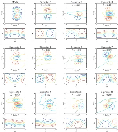
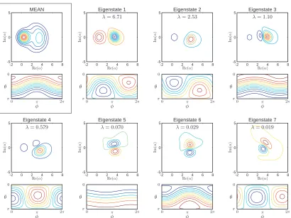
Proper Orthogonal Decomposition (POD), alternatively known as Principal Component Analysis or the Karhunen-Lo`eve decomposition, is a model-reduction technique which generates the optimal linear subspace of dimension D for a given set of higher-dimensional data. That is, if the data are contained within an attractor, the POD process can produce the affine linear space that best approximates the space containing that attractor. In this Chapter, I give a short derivation of the POD algorithm, then show the results from applying it to two different bistable atom-cavity regimes. For each regime, I show the performance of filters based on these POD results.

3.1 Background

The Proper Orthogonal Decomposition (POD) process has been derived in a variety of fields, which has resulted in it having several names. In fluid dynamics, it is known as the Karhunen-Lo`eve decomposition, and has its origins in the work of Lumley [28]. The method itself had its origins in Pearson [29] and again in Hotelling [30].

The derivation which follows is based on those presented by Lallet al. [31] and Zhang and Zha [32]. We start with an empirical set of data — an unordered collection ofN pointsx(i)_in_Rm_{. In the}

cases to be examined below, these will be vectorized forms of the density matrixρ. We would like to build the optimald-dimensional affine subspace ofRm, which will be isomorphic to Rd. Zhang and Zha take the approach of building the optimal map from the lower dimensional space to the higher, while Lall et al. choose to find the optimal projector from the larger space to the smaller. Here I choose the latter path, because it is more consistent with our goal of projecting the dynamics into the lower-dimensional space.

We would like to find the optimal projection matrix, Q∈Rm×m_{, from} _Rm _{to a} _d_-dimensional

(40)

distance of the original set of points from thed-dimensional plane:

E(Q) =

N

X

i=1

kx(i)−Qx(i)k2. (3.1)

We wish to find the optimal affine subspace, which must go through the mean of the data, so we subtract the mean of all thex(i)_{s, ¯}_x_{, from each point before proceeding. We next construct the}

correlation matrix

R=

N

X

i=1

(x(i)−x¯)(x(i)−x¯)∗_, _(3.2)

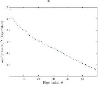
and calculate its eigenvalues, orderedλ1≥λ2≥ · · ·λm. It is then a standard result that

min

Q E(Q) =

m

X

l=m−d+1

λl. (3.3)

The magnitude of each eigenvalue measures the relative contribution of the direction corresponding to the paired eigenvector to the data distribution as a whole. By cutting off the space atddimensions, we measure the error,E, by summing the eigenvalues corresponding to the directions we have chosen to discard.

Turning now to constructing the projector into this optimal subspace, we make use of the or-thonormal eigenvectorsφ1, φ2, . . . φd corresponding to the largest eigenvalues. The approximate ˆx(i)

tox(i)_{is given by}

ˆ

x(i)=

d

X

j=1

aijφj+ ¯x (3.4)

where

aij=

D

x(i)−x, φ¯ j

E

. (3.5)

Now denote by P the d×m matrix whose rows are φ1, φ2, . . . φd. Then the approximant to x is

P∗_P₍_x₋_x_¯_{) + ¯}_x_{, and}_y₌_P₍_x₋_x_¯_{) are the new coordinates for}_x_{in the new,}_d_{-dimensional subspace.} In this derivation, we have assumed ana priori known, fixed,d, but in practice one constructsR, and then examines its eigenvalues, choosingdsuch that the error (3.3) is below whatever threshold one decides.

3.2 Proper Orthogonal Decomposition of quantum

trajecto-ries

(41)

Orthogonal Decomposition. Applying the POD process to quantum trajectories requires making a few, nontrivial choices. What space will we define as the larger space of which we seek the optimal subspace? What is the appropriate measure of distance between states, to evaluate the error and optimality of the subspace? A quantum trajectory, in order to be computationally tractable, requires measurement of every output, meaning that states remain pure at all times. We therefore start with wavefunctions, rather than density matrices. However, we know that the experimentalist will almost never have full observation of their system, meaning that she will be working with density matrices.

Density matrices have an amenable algebra, with a clear inner product

hρ1, ρ2i= Tr(ρ1ρ2) (3.6)

for use in Eqn. (3.5). In addition, the form that a “direction in density matrix space” will take is clear: a trace-0, Hermitian matrix. For small perturbations of a density matrix by addition or subtract of such a matrix, we know the resulting matrix will almost always remain a valid density matrix — trace 1, positive, and Hermitian. We will see below that large perturbations can result in non-physical density matrices. In contrast, it is not clear how to define a “direction in wave function space.”

Of course, the POD algorithm requires its input to be vectors, in order to calculate the correlation matrixR. My process was to create the density matrix corresponding to each wavefunction, ρi =

|ψiihψi|, and then to “vectorize” each density matrix. Rather than simply creating a vector which was

the end-to-end concatenation of each row or column ofρi, I took advantage of the Hermitian structure

of the matrix to make a completely real vector by first concatenating the real parts of the rows of the upper-triangular portion of the density matrix, and then concatenating that with the imaginary parts of the upper-triangular portion (aside from the diagonal, which is entirely real). This significantly simplified the computer code necessary to implement the algorithm, and eliminated the chance of error due to confusion of which transpose operations should be complex-conjugate transpositions, and which should be simple transpositions. The ∗ _{operations in the derivation above are complex} conjugate transpositions, but derivations in the literature are not specific on this point, as they assume that everything is simply real. In practice I verified that if one simply unwraps the density matrix, leaving its vector form complex, and treats these as complex-conjugate transpositions, one achieves the same results as I do with the less-mistake-prone real-only method.

Reduced Order Models for Open Quantum Systems