University of London
Path-dependent functionals of Constant Elasticity
of Variance and related processes: distributional
results and applications in Finance.
Jayalaxshmi Nagaradj asarma
London School of Economics and Political Science
A thesis subm itted in partial fulfillment of the requirements for obtaining the degree
of Doctor of Philosophy
UMI Number: U 613350
All rights reserved
INFORMATION TO ALL U SE R S
The quality of this reproduction is d ep en d en t upon the quality of the copy subm itted. In the unlikely even t that the author did not sen d a com plete m anuscript
and there are m issing p a g e s, th e se will be noted. Also, if material had to be rem oved, a note will indicate the deletion.
Disscrrlation Publishing
UMI U 613350
Published by ProQ uest LLC 2014. Copyright in the Dissertation held by the Author. Microform Edition © ProQ uest LLC.
All rights reserved. This work is protected against unauthorized copying under Title 17, United S ta tes C ode.
ProQ uest LLC
789 East E isenhow er Parkway P.O. Box 1346
T h £ S £ S
F
S 2 i 6
POLITICAL
A cknow ledgem ent
First and foremost, I would like to thank my supervisor, Dr Angelos Dassios for
his encouragements, his patient guidance, his resourceful advice and his permanent
availability in helping me to overcome the difficulties th a t arouse during the course
of this research work.
I would also like to thank Pr. Ragnar Norberg and Pr. Riidiger Kiesel for their
comments and suggestions offered during my presentations at the Department of
Statistics seminar. I am also grateful to Dr Chacko and Dr Das for answering some
of my questions regarding their research work on average-rate claims.
I am grateful for the financial support the Departm ent of Statistics of the London
School of Economics has given me through the LSE Research Studentship.
To my friends and office mates, Diego, Panos and Yorghos, evxc^pi'O'TU for your help, your ability to cheer me up when needed and your friendship. Also thank you
to Simona and Teresa whose seniority made them play a scout role for me.
To my husband, I would like to address a special thanks for his encouragements
and love and for having beared with me regular travelling and separation. To my
parents who supported me in all possible ways each and every day, I want you to
know th a t it is your support and your faith in me which helped me through the years.
A b stract
The present thesis provides an analysis of some path-dependent functionals of Constant Elasti
city of Variance (CEV) processes. More precisely, we study the continuous arithmetic average of the
process over time, plain or sometimes multiplied by a knock-out indicator. We start by describing
its mathematical properties and provide new distributional results (moments, densities, moment
generating function among others). Some of these results also pertain to the joint distribution of the
integral and the process itself. The versatility of the process enables us to consider diverse financial
applications: fixed and floating strike Asian options on equities, European vanilla options on equity
in the presence of stochastic volatility as well as zero-coupon bonds, guaranteed endowment options
and average-rate claims under stochastic interest rates.
We devote a great part of the present work to the square-root process and the geometric Brownian
motion, two important subcases of the CEV process. For both these nested diffusions, a number of
mathematical and financial quantities have been solved for in the literature in closed-form, in terms
of Laplace transforms. In this thesis, we derive these quantities in a fully explicit form, which is
advantageous both from a theoretical point of view, to gain insight in their mathematical structure
and from a practical stand, as the numerical evaluation of our formulae appear more robust and
efficient than other numerical methods for some ranges of parameters. In the general CEV case, for
which the integrated process has scarcely been considered in the literature, we derive semi-closed
C ontents
A ck n ow led gem en t i
A b stra ct ii
In tro d u ctio n 1
1 D istrib u tio n a l resu lts 8
1.1 The square-root process ... 9
1.1.1 Study of the p r o c e s s ... 9
1.1.2 The joint moments of (Xt, T t ) ... 16
1.1.3 The joint density of (Xf, F t ) ... 21
1.1.4 The marginal density of the integral in the mean-reverting case 30 1.2 The geometric Brownian m o tio n ... 40
1.3 The general CEV p ro cess... 42
1.3.1 The equity CEV m o d e l... 42
1.3.2 The integrated p r o c e s s ... 45
1.3.3 Numerical illu s tr a tio n s ... 52
1.4 C onclusion... 54
1.5 Appendices to this c h a p te r ... 54
1.5.1 Proof of Theorem 1 .1 .9 ... 54
1.5.2 Proof of Theorem 1 .1 .1 0 ... 62
2 A sian op tion s on stock s 66 2.1 Literature review of Asian o p tio n s ... 67
2.1.1 The different types of Asian o p tio n s ... 67
2.1.2 The different approaches carried out ... 70
2.2 The classical lognormal c a s e ... 75
2.2.1 A linear SDE of i n t e r e s t ... 75
2.2.2 Hitting time MGF ... 78
2.2.3 An alternative derivation of the Laplace transform of fixed-strike Asian options ... 81
2.2.4 Analytical inversion of the Asian Laplace transform: Bromwich integral and residue calculus... 83
2.2.5 Eigenfunction expansion technique: explicit integral form. . . 87
2.2.6 Eigenfunction expansion technique: series form... 94
2.2.7 Numerical a p p lic a tio n s ... 102
2.2.8 An excursion to jum p-diffusions... 105
2.3 The square-root process c a s e ... 109
2.3.1 Preliminary r e s u l t s ... 109
2.3.2 The distribution of P r ... 112
2.3.3 Fixed strike Asian o p tio n ... 114
2.3.4 Numerical illu s tra tio n s ... 116
2.4 C onclusion... 118
2.5.1 Call option on an absolute-dividend paying stock: Proof of The
orem 2 . 2 .5 ... 119
2.5.2 Square-root Asian option: proof of the preliminary Theorem 2.3.2121 2.5.3 Square-root Asian option: proof of the preliminary Theorem 2.3.3 for a b s o rp tio n ... 126
2.5.4 Fixed strike Asian option: proof of Theorem 2 .3 .6 ... 127
3 In terest rate d erivatives 129 3.1 The Cox Ingersoll Ross m o d e l ... 130
3.1.1 In tro d u c tio n ... 130
3.1.2 Preliminary r e s u l t s ... 133
3.1.3 Probability distribution function of the cumulative interest rate 142 3.1.4 Truncated expectation of th e cumulative interest r a t e ... 142
3.1.5 G uaranteed endowment o p tio n ... 143
3.1.6 Binary Asian o p tio n s ... 144
3.1.7 Regular Asian o p t i o n s ... 145
3.1.8 Numerical r e s u l t s ... 147
3.2 The CEV model for the instantaneous r a t e ... 151
3.2.1 A Laplace transform a p p ro a c h ... 152
3.2.2 Considering an eigenfunction expansion a p p r o a c h ... 156
3.2.3 Numerical e x a m p le ... 157
3.3 C onclusion... 158
3.4 Appendices to this c h a p te r ... 160
3.4.1 Proof of Theorem 3 .1 .1 ... 160
4.1 Reference m o d e l s ... 169
4.1.1 The Hull-W hite m o d e l ... 169
4.1.2 The Stein and Stein m o d e l... 171
4.1.3 The Heston model ... 173
4.1.4 Moment generating\characteristic functions approaches . . . . 176
4.1.5 Revisiting the Hull-White model ... 180
4.2 Moment based approxim ations... 181
4.2.1 Moments for the reference m o d e ls ... 182
4.2.2 Hull-W hite type of a p p ro x im a tio n s ... 184
4.2.3 Volatility of volatility e x p a n sio n ... 186
4.2.4 Edgeworth e x p a n sio n ... 187
4.2.5 Laguerre polynomial e x p a n s i o n ... 190
4.2.6 A small parenthesis on bounded v a ria n c e ... 192
4.3 Numerical c o m p ariso n s... 195
4.4 C onclusion... 198
4.5 Appendices to this c h a p te r ... 198
4.5.1 Stein and Stein model: functions d e f in itio n s ... 198
C on clu sion 200 A Special fu n c tio n s 204 A.0.2 Hermite p o ly n o m ia ls ... 204
A.0.3 Hermite polynomials of the second k in d ...205
A.0.4 Laguerre polynom ials... 205
A.0.5 Gamma fu n c tio n s ...206
A.0.7 Parabolic cylinder f u n c tio n s ... 208
A.0.8 Bessel fu n c tio n s ... 209
B N u m erica l L aplace tran sform in version 210
C E ig en fu n ctio n exp an sion 212
List o f Tables
1.1 Evolution with y at x = 100... 29
1.2 Evolution with t at x = 100 and y — 102.54... 29
1.3 Evolution with (j at x — 100 and y = 102.54... 29
1.4 Evolution with ^ at a; = 100 and y = E iX t)... 30
1.5 Evolution with time (base parameters: a = 0.15, b = 1.5, a = 0.2 and Xq = 0.1) ... 37
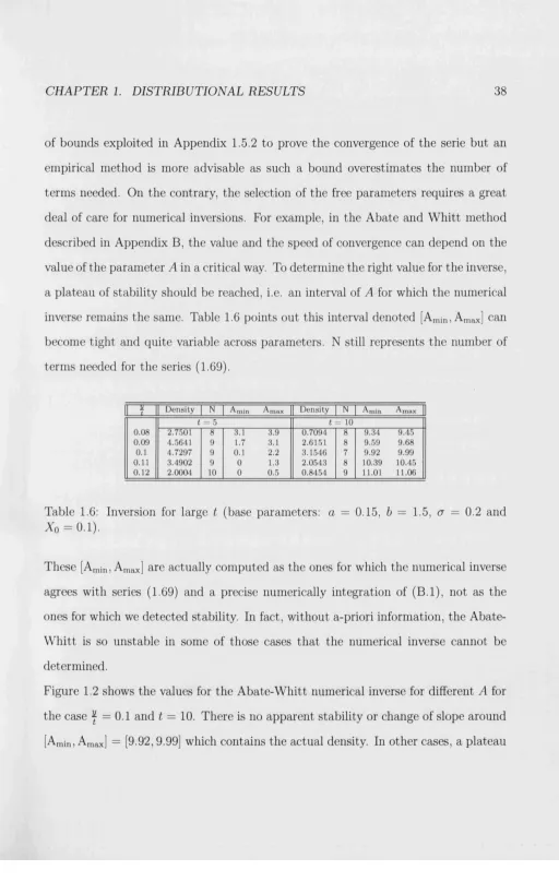
1.6 Inversion for large t (base parameters: a = 0.15, 6 = 1.5, <j = 0.2 and Xo = 0.1)... 38
1.7 Inversion for a = 0.3 and t = 1... 39
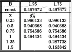
1.8 Evolution of the basis functions with respect to r o ... 52
1.9 Evolution of the approximate Laplace transform for different B . . . . 52
2.1 Fixed-strike Asian options, explicit integral fo rm ... 102
2.2 Floating-strike Asian options, explicit integral f o rm ... 102
2.3 Fixed-strike Asian options, approximate series f o rm ...103
2.4 Evolution of the location of the zeroes with respect to B ... 104
2.5 Fixed-strike Asian options... 116
2.6 Evolution with the m a tu rity ... 117
2.7 Evolution with the volatility... 117
2.8 Evolution with the strike... 118
3.1 Evolution with T, Chaeko and Das param eters... 147
3.2 Asian options on yield... 148
3.3 Higher maturities, Chacko and Das param eters... 149
3.4 Evolution of the speed of convergence with T ... 149
3.5 (7 = 0.3, T = 1, Chacko and Das param eters... 151
3.6 I = 0.05, T = 1, Chacko and Das param eters... 151
3.7 Evolution of the basis functions with respect to r o ... 157
3.8 Evolution of the approximate Laplace transform for different B . . . . 158
4.1 Volatility of volatility expansion... 196
4.2 Edgeworth expansion... 197
List o f Figures
1.1 So = 100, a = 0, b = —0.05, <j == 2 and t = 1 28
1.2 Instability of Abate-W hitt numerical inverse... 39
1.3 Evolution o f the transform with respect to fi at X = 1... 53
1.4 Evolution o f the transform with respect to X at p, = 1... 53
2.1 The Bromwich c o n to u r... 85
2.2 Evolution o f the speed o f convergence with respect to B ... 104
3.1 ro = 0.1, a = 0.15, b = 1.5, a = 0.2 and T = 1 0 ... 150
In trod u ction
Option pricing theory - an endeavor to reduce the likelihood of being fooled by randomness, as Nassim Taleb would claim, but also a fascinating field with a relatively long history. By 1900, Bachelier first suggested a fair game approach to a
world driven by a gaussian underlying security price, suspicious idea when examined
under the utility and risk-aversion theory light. Shouldn’t an option be worth less
than its fair value for a risk-averse individual? This puzzle was solved only seventy-
three years later by Black and Scholes who proved th a t a call option can be perfectly
replicated by a self-financing portfolio of cash and asset under the assumption th a t the
security follows a geometric Brownian motion with constant volatility, th a t there is no
short-selling constraint and no transaction cost and finally th a t absence of arbitrage
opportunity prevails. Their work represents the cornerstone of financial m athem atics
and the ulterior option pricing results derived under the same set of assumptions
have generally - respectfully or affectionately - referred to this model as the Black-
Scholes environment. Most of the subsequent research has been heading towards
either relaxing one or more of these basic assumptions, specially the distributional
hypothesis (jump diffusion: Merton [55], etc., constant elasticity of variance processes:
Cox and Ross [16], Beckers [6], etc., stochastic volatility models: Hull and W hite [41],
complex exotic or path-dependent instruments (barrier options: Merton [54], etc.,
lookback options: Goldman and al. [36], occupation time derivatives: Dassios [20],
etc.).
In the present work, we focus on path-dependent functionals of constant elasticity
of variance (called CEV hereafter) processes, more precisely on tem poral integrals
of these processes, either unrestrained or constrained by a knock-out condition, i.e.
multiplied by the indicator of the underlying process not reaching a given high level
before some m aturity date. The versatility of the CEV process enables us to develop
applications in different main branches of m athem atical finance, since it has been
used to model equities, interest rates and other stochastic volatilities.
Our analysis, i.e. this thesis, is constituted of four chapters. The first and most
general one collects a summary of the distributional attributes and a thorough ana
lysis of the CEV processes. We first deal with the square-root process as it could be
hailed as the root or rather the common ancestor of all the processes encountered in
this thesis. Indeed, both the CEV process of elasticity strictly less th an unit and the
geometric Brownian motion originate from the square-root process through a power
transformation and respectively a random time-change. We therefore devote a major
part of the chapter to the square-root case. After getting better acquainted with the
Feller [29] process itself by studying its different m athem atical properties, we present
various new results pertaining to the integrated process, starting w ith its moments.
The moments have been used in the literature, typically for stochastic volatility mo
dels (see Ball and Roma [5] for example). However, they are usually obtained by
successive differentiation of the moment generating function of the integral - which
moments of the process and its integral are expressible as a polynomial of exponen
tials and powers of time whose coefficient can be computed with a simple recursion.
We also show th a t knowing these moments is of param ount importance since they
determine the joint distribution. Though this result theoretically enables us to ex
press a great number of quantities related to the integral, we prefer a more direct
approach to the issue of determining the joint distribution and to this effect, employ
the joint moment generating function (abbreviated as MGF throughout the thesis) of
the process and its integral as our starting point. It turns out th a t the problem boils
down to considering the - relatively simpler - corresponding squared Bessel process,
since we prove th at a general square-root process can be brought back to its squared
Bessel counterpart with an appropriate change of measure. Other links between these
processes have been provided in the literature. Yet, our change of measure result is
stronger in the sense th a t it allows to study path-dependent properties in a simple
way. It noticeably enables us to derive the joint distribution as an explicit series,
both for the mean-reverting and the non mean-reverting case, which needs a careful
treatm ent to account for the absorption at the origin. This formulation turns to be
quite simple for the non mean-reverting case. However, a simpler expression can be
obtained for the marginal distribution of the integral in the mean-reverting case from
a different construction of the inverse Laplace transform of the moment generating
function. All of these results are novel to the best of our knowledge and have a number
of applications, some of which are discussed in the following chapters. Having tho
roughly examined the square-root case, we move to another im portant subcase, the
geometric Brownian motion case and then to the general CEV process. For the Geo
metric Brownian motion, we will only present an overview of the research developed
options rather than deriving results on the already well-studied distribution itself.
All our new results concerning this process are therefore left to be presented in the
second chapter. We finally study the general CEV case for elasticities strictly between
0 and 1. Showing how they relate to the square-root process, we deduce a number of
properties, among which a generalisation of the change of measure which simplifies
the diffusion equation in the square-root case. We then attem pt to characterise the
distribution of the integrated process through its moment generating function. Under
the least restrictive hypothesis th at the elasticity is a rational number, we provide an
expression for the Laplace transform with respect to time of the moment generating
function resulting from a second-order inhomogeneous differential equation. This ap
proach has never been attem pted before, to the best of our knowledge, and helps us
to gain insight into the m athem atical structure of the problem.
The second chapter focuses on the pricing of Asian options on equities, deriva
tives of considerable importance both for market practitioners and financial theorists.
Asian type of options are advantageous treasury management tools as well as safer
structures for thinly-traded assets whose price could be hugely impacted by one large
enough market participant. They are also renowned as one of the most difficult to
evaluate path-dependent options as testified by the concentration of research and
diversity of approaches explored for this problem. We concentrate on continuous
arithm etic averages, i.e. underlyings related to the temporal integral of the process.
Given the richness of the field, a review of the various results and main techniques
proposed in the literature appears a compulsory step and is carried out first. We
then explore the most commonly adopted model, the geometric Brownian motion,
i.e. the Black and Scholes environment. Our contribution consists in the derivation
We provide as well a synthesis of different formulations reducing the problem to a
one-factor Markovian one, either by time-reversal arguments or by working under the
asset-numeraire. Along these lines, we present a simple alternative derivation of the
Geman and Yor [77] Laplace transform of the Asian call price, methodology later generalised to handle jum p processes. We then invert analytically this Laplace trans
form by contour integration for different types of options. A second approach, which
is to bound the state space by absorbing the process at a high level, enables us to
derive these prices as an eigenfunction series instead of an integral. We finally show
how these Laplace transforms can be modified under the extended model including
multiplicative jumps on the underlying, which completes our study of the geometric
Brownian motion case. In the last part of this section, we show th a t simpler ex
plicit solutions can be obtained under the alternative square-root model of Cox and
Ross [16] as an application of the results derived in the first chapter. This makes this
model quite interesting for testing and risk-management purposes.
Interest rates derivatives are another main branch of application and the subject
of Chapter 3. The Cox Ingersoll Ross [15] (CIR) model based on a square-root
process for the instantaneous rate constitutes a benchmark model for its combined
tractability and adequacy to what is expected from a short rate process evolution.
This model is generally labeled as tractable for the existence of an explicit formulation
for bond prices. Yet, a number of other derivatives can only be obtained in term of
Laplace transforms. The distributional results derived in the first chapter allows
us to further the analysis of this model and provide explicit prices for guaranteed
endowment options as well digital and regular average-rate claims. As any interest
rate derivative depends on the cum ulated rate, other applications could be considered
and Sanders [13] popular and empirically validated model featuring the short rate
as a CEV process. Unlike in the CIR case, no explicit solutions could be given.
We however extend the results of the first chapter on equities CEV and propose
a semi-closed expression for the Laplace transform of the zero-coupon bonds prices
with respect to the maturity. A fast Fourier inversion of this transform would be an
effective solution when a whole yield-curve is needed, as often happens in practice.
The fourth chapter takes us back to the equity world. However, instead of consider
ing elaborate path-dependent derivatives, we will study standard vanilla options under
more complex models including stochastic volatility. The classical stochastic volatility
processes considered in th e financial literature are typical subcases of the CEV pro
cess: Geometric Brownian motion for the Hull-W hite model [41], Ornstein-Uhlenbeck
for the Stein and Stein [67] model and square-root process for the Heston [40] model.
Synthetising these original models first, we propose an intuitive way of using moment
generating and characteristic functions to recover very simply the characteristic func
tion of the log-asset under the last two models. We also extend this methodology to
derive novel close-form solutions for the Hull-White case. We then focus on moment-
based approximates for the options prices, first by extending and comparing several
approximation previously proposed for the Hull and W hite model and then by finding
convergent series based on polynomial expansions.
A couple of remarks should be added before finishing this introduction. Except for
the distributional hypothesis in some cases, all the standard assumptions of the Black
and Scholes world hold throughout this thesis, namely, no short-selling constraint,
no transaction cost and no free-lunch. We work on a probability space (f^ ,P ,^ )
and always place ourselves under the risk-neutral measure unless otherwise specified.
measure. The work of Harrison and Kreps [39] then equates the value at tim e t of any derivative with the expectation of its payoff conditionally on ^ under the risk-neutral
measure. All the option prices handled in this thesis are derived as such expectations.
We finally wish to point out some abbreviations used throughout this thesis, some
of them have already been defined in this introduction. We abbreviate Constant
Elasticity of Variance by CEV, Moment Generating Function by MGF, Stochastic
Differential Equation by SDE, Partial Differential Equation by PD E and Ordinary
C hapter 1
D istrib u tio n a l resu lts
The popularity of the CEV process in all main branches of financial modelling
can be explained by its desirable property of positivity and its richness of behaviour:
indeed, depending on its parameters, the process can be mean-reverting or exploding,
the boundary at 0 can be absorbing, refiecting ... It has been used to model equities,
interest rates, stochastic volatility and other financial quantities. Our goal, here, is
to derive some properties and distributional results for these processes.
We first consider the square-root process, which is the most tractable since it allows
for fully explicit formulations for various quantities. It is also closely linked with the
more general CEV process, as explained in the introduction. We start by presenting
some of the main properties of the square-root process given in the literature. We
then derive the joint moments of the process and its average. The average moments
have indeed an im portant informational content, since they are proven to actually
determine the distribution of the average. A more direct approach yet allows us
to determine in a more efficient way the joint distribution of the process and its
C H A P T E R 1. D ISTR IB U TIO N A L RESU LTS 9
relating the square-root process to its square Bessel process counterpart. We then
proceed to find a simpler expression for the marginal distribution of the average in
the mean-reverting case. This completes our study of the square-root case. We then
present the main classical results concerning the distribution of the tem poral integral
of a geometric Brownian motion. Finally, we turn to the general CEV process for
elasticities strictly between 0 and 1 and attem pt to solve for its moment generating
function under the non restrictive assumption th at the elasticity is a rational number.
1.1
T he square-root process
Defining first the notations used in this section, X t will represent a smooth version of the square-root process following the stochastic differential equation:
dXt = {a — bXt)dt P a y jX td W t (1.1)
with (a, a) G M'*' x R+ and 6 G M.
The next part of this section collects a number of im portant properties of X t, some of which are well-known^ but need to be recalled to provide a deeper understanding
of the process structure. X t may sometimes be referred to in the following as the spot (for spot-rate or spot-equity) whereas the temporal integral Yt = / J Xgds will often be called the integrated process.
1.1.1
S tu d y o f th e process
The first and foremost issue to consider when studying a diffusion remains the actual
existence and uniqueness of such a process.
C H A P TE R 1. D ISTRIBU TIO N A L RE SU LTS 10
i. Strong so lu tio n
P ro p o sitio n 1.1.1. (see Feller [29], Lamberton-Lapeyre [46]) For any positive x q ,
there exists a unique continuous adapted process X t satisfying the stochastic differen tial equation (1.1) and the initial condition Xq = x q .
P ro o f. Though the usual Lipschitz condition is not satisfied by the local volatility of the equation (1.1), the square-root function is locally holderian. Adding th at the
drift coefficient is locally Lipschitzian, existence and uniqueness of a smooth version
are ensured (see the references in Lamberton and Lapeyre [46]). □
ii. T h e zero-b ou n d ary
Positivity is a very well-known (and for modelling purposes, a generally apprecia
ted and useful) property of the square-root process. But, for a proper understanding
of the process, its behaviour at 0 needs to be analysed.
P ro p o sitio n 1.1.2. (see Lamberton-Lapeyre [46]) I f a > ^ , 0 is an entrance bound ary, i.e almost surely, the process will not reach 0 in finite time^. I f a = 0, 0 is an absorbing boundary. Then, if b > 0, the process will almost surely get absorbed in finite time. I f b < 0 , the absorption probability lies strictly between 0 and 1.
P ro o f. A proof of all these results can be found in Lamperton and Lapeyre [46]. □
iii. T h e lim it-d istrib u tio n in th e m ean -revertin g case
It appears from the previous result th a t the process behaviour depends crucially
on the sign of b. Indeed, a strictly positive b induces the process to mean-revert to
"^Except when Xq = 0, in which case the process automatically departs from 0 and never get back
C H A P T E R L D IST R IB U T IO N A L R E SU L T S 11
the level | and convergence with time to a stationary distribution can be expected.
Therefore, whenever positive and non-null, b will be thereafter denominated the mean- reversion strength.
P r o p o s itio n 1.1.3. (see Shreve [66]) W henb is strictly positive, the process converges with time to the gamma distribution
\ %
26 r 1
x ~ ^ e ~ ^ (1.2)
r(H)
P ro o f. If such a equilibrium-distribution exists, it has to be the solution of
+ (a - <7^ - b x ) ^ - b p M = 0 . /o°° P<x,(x)dx = 1
with the the constraint Poo(^) > 0,V?/ > 0.
(1.3) arises from taking the limit when tim e tends to infinity of the Kolmogorov
forward equation
^ “ b x ) p { t , x ) ) - - — { a ‘^ x p { t , x ) ) = 0
given th a t for a distributional limit to exist, the following condition should be satisfied
i t a £ p | £ ) = o t-KX) Ot
Note th a t the forward equation represents here a natural choice compared to the
backward one, since the limit distribution should be independent of the starting
values, i.e. the backward variables xq and to, implying th a t taking the limit in time of the Kolmogorov backward equation would provide no information.
The basis for the vector space of solutions being
C H A P TE R 1. D ISTR IB U TIO N A L RESU LTS 12
The second function, which can be rewritten as p2 = is the only
integrable solution over R+ and is also clearly positive. Normalising it by its integral
leads to (1.2).
This convergence in distribution can be actually proven by taking the limit in
infinite time of the moment generating function of X t which will be given in the next
subsection in Proposition 1.1.4. □
R em ark. When b is negative, on the other hand, the MGF does not converge and
the first moments of the process are easily shown to grow to infinity with time.
iv. T h e join t m o m en t-gen eratin g fu n ction
The first and actually main results concerning the tem poral integral Yt = /q Xsds
have been derived by Cox and al. [15] in their com putation of the price of a zero-
coupon bond. Their result can easily be generalised to obtain the moment generating
function of Yt. W ithout heavy complication, the same method actually produces the MGF of the joint distribution {X t,Y t) as observed, for example, by Lamberton and Lapeyre [46]. The (relative) simplicity of these functions comes from the additivity
property of the process. This same tractability of solutions of linear (or rather affine)
differential equations have given rise to the so-called affine models.
P ro p o sitio n 1.1.4. The moment generating function o f the jo in t distribution o f
(X t,Y t) has the exponential form
n) = = xo) = (1.4)
with
C H A P TE R 1. D ISTRIBU TIO N A L RESU LTS 13
and
where
—2 f 27e 2^^*
Va2A(l - e - ^ ) + (7 + 6) + e"i'*(7 - h) ^
7 = y/h"^ P 2/x<j2 (1.7)
P ro o f. This proof is included both because of the importance of the result and because of the development of the proof itself, which might be useful to be compared
with related results we will derive later in this thesis for the CEV process.
Consider L{t, x), the bounded solution of the following partial differential equation
dL d'^L , ^ ,d L ~
a ï - T W + subject to the initial condition
L{0,x) = e - ^
The process
M( = - 1, X t)
is then a martingale and this implies
L ( T ,X t ) = Mo= E ( M t) = = L{X,n)
As in Corollary (1.3), Chapter 11 in Revuz and Yor [62] ( See also Pitm an and Yor [60] and Shiga and W atanabe [70] ), the solution has the form L{X,(jl) =
The sum of two independent square-root process with parameters a^, 6, cr and a‘^,b ,a
respectively and initial values x j and Xq respectively is a square-root process^ of
CH APTE R 1. D ISTRIBU TIO N A L RESU LTS 14
parameters a and initial value Xq-\-Xq. The joint MGF for the process with parameters a, b, a and xq is hence the product of the joint MGF for a square-root process with parameters 0 ,6, a and xq and the joint MGF for an independent square-root process with parameters a, 6, a and initial value 0. Each of these two MGF are multiplicative and equal to 1 at 0.
The differential equation then becomes
ü T { t ) = X + T ^ ( ^ ) - |- 6 T ( ( ) —
giving the following system
e'(t) =
m
(1,8)
_ V ( t ) = - 6T(«) + with the initial conditions 0(0 ) = 0 and T (0) = A.
The last equation in (1.8) is a ordinary Riccati differential equation, with the
constant particular solution: Tq = -b+y/b^+2^ W ith 7 defined as in (1.7), the
change of variables: h{t) = Y(tf-ro le&ds to
2
h'{t) = — + (ct^Tq -f b)h{t)
and
1
h{0) =
A — To
which result in the expressions (1.5) and (1.6). □
V. T h e d en sity o f th e sp o t-p ro cess
Although the MGF completely characterises a distribution in theory, its density
remains in practice most desirable since needed, for instance, to compute the expec
CH APTE R 1. D ISTRIBU TIO N A L RESU LTS 15
T h e o re m 1.1.1. The square-root process density is an infinite weighted average of gamma densities. In the non-absorption case,
f ^ i x ) = e -^o B e - g (1 9 )
where
Feller [29] represents it in the equivalent form
= (1.11)
where 12 ^ - 1 is the modified Bessel function of the first kind of order | l — 1*
This density corresponds to a non-central chi-square with ^ degrees o f freedom and parameter of non-centrality 2Bxoe~^^.
R e m a rk . Besides the intrinsic importance of this result, the proof given below is
of specific interest as it illustrates the analytic Laplace transform inversion method
which consists in decomposing the transform into a sum or a series of elementary
analytically invertible terms, method widely used in this thesis.
P r o o f o f T h e o r e m 1 .1 .1 . Taking // = 0 in (1.6) and (1.5), leads to the MGF of
" "I
( 1.12) can be rewritten as
C^(X) = I
00 n / R \
C H A P TE R 1. D ISTR IB U TIO N A L R E SU LTS 16
Given th a t (A + a)~'' is the MGF of the gamma distribution of density
the linearity property of Laplace transforms along with the Beppo Levi monotone
convergence theorem applied to this weighted sum of (positive) densities allow the
inversion (1.9). The equivalence with (1.11) follows from the series representation of
the Bessel function
oo / \' ^ + 2 *
(
21
□
This is the first result in this chapter involving Yt. Our interest for this quantity is rooted in its importance as a financial underlying. But, if, for some derivatives,
the price depends only on the marginal distribution of the average, the spot enters
as well the payoff of some other derivatives, in which case the joint density might be
needed We will therefore first study the joint distributional properties of (Xt,Yt),
starting with their moments.
1.1.2
T he join t m om ents o f
{Xt,Yi)
In the literature concerning stochastic volatility, the moments of the average have
been used either to compute approximations for the price (see Ball and Roma [5]) or to
gain insight in the distribution of the stock (see Das [19]). However, only the four first
moments have been given in these texts since they were computed through successive
differentiation of the moment-generating function. Though it is theoretically possible
to obtain all these moments through repeated differentiation, this method remains
tedious and even with formal calculus packages like M athematica or Maple, only the
first ones can be handled in this quite time-consuming way. We show here th a t it is
C H A P TE R 1. D ISTR IB U TIO N A L RESU LTS 17
actually possible to obtain all of them analytically, since it turns out th a t they have
a relatively simple form.
i. T h e jo in t m o m e n ts in e x p lic it fo rm
T h e o re m 1.1.2. The joint moments o f X t andYt are given by
j m , n
= E i Y r x r n =
È
(115)where
I p ^ = m in(n + 1 — j, m + 1) (116)
The coefficients 3,1' can be obtained by recursion through the relations • For j ^ n — m
a , ■ = m
E
“ ( { n - m - j)by-'^+^
For j = n — m
o For i = 1
n ^n—m TTl—l , n
/ 2 \ n —m m , 7 l —1
+(n
-m)(a + {n-m-
Dy) g E
+
3='
o For 2 > 1
C H A P T E R 1. D IST R IB U TIO N A L RE SU LTS 18
where
C m, n = r o l { m = 0 } ( 1 - 2 0 )
• Initial condition
û;o;Î = 1 (1-21)
R e m a rk . The marginal moments of Yt are obtained with n = m , since E{Yt^) =
A I n , n { t ) '
P r o o f o f T h e o re m 1 ,1 .2 . Assessing first the issue of existence, the joint MGF
given in Proposition 1.1.4 is infinitely differentiable in a neighbourhood of (0,0) ,
implying the joint moments of X t and Yt exist for any positive order for any finite t . Therefore, applying the Ito formula to Y ^X !^, taking the expectation of the result and differentiating it with respect to t gives
2
-bkE{Yt"^X^) + k (k - l ) y E ( y ( ” ‘X * - ‘ ) ( 1 . 2 2 )
since the stochastic integral appearing when applying the Ito lemma is a martingale,
due to the square-integrability property of the integrand formed by power functions.
It should be noticed th a t the com putation of positive order moments does not actually
involve the moments of the reciprocals of either or W hen m = 0 or respectively A: = 0, the use of m E {Y ^ ~ ^ Xt'^^) and respectively k E {Y /^X t~ ^) are mere notations let for simplicity while those expectations do not in fact appear in the equation and
the term s quoted are simply null.
Now, denoting Mm,n{C) the Laplace transform of = E { Y ^ X t~ '^ ) w ith respect to time for ( G R+, M m,n{0 = €T^^Mm,nit)dt , the ordinary differential equation (1.22) becomes
C H A P TE R 1. D IST R IB U TIO N A L RE SU LTS 19
with
d{n,m ) = {n — rn )^a -\-{n — m — 1 ) ^ ^ (1 24)
(1.15) can then be shown trough induction. Assuming th at for a given n > 0 and for
all integers m < n, the joint moments have the form
n —1 L ’ m ,n —1
The Mk,n are also assumed the corresponding form for all k strictly below a given integer m > 0, whenever m > 0. As in (1.20), defining the variable Cm,k by co,k =
and Cm,k = 0 if m > 0, (1.23) implies that^
jTfVfTl jTTl — 1 ,Tl
n ■'i m,7i N m - l , n
j , i Cm,n _ ^ j , i________
^
+
M Ç + b { n - m )^
^
(C +
jbYiC+
b(n - m))r ? n ,n —1
n — 1 771— l , n
E M Ë W z # ) < * ■ “ >
Given th at, for p g positive integers,
1 _ /ÎÎ.. ,
(1.27)
(C + 96)‘(C
+ vb)
(,+pb
^ (C + gf»)'
with
~ (g-p)fc
(1.26) and (1.27) leads to the recursions (1.17), (1.18) and (1.19).
Since (1.25) is clearly initially satisfied for (m, n) = (0, 0) with Mo,o = ^ (explai
ning (1.21)), the Mo,o = ^ have the form given in (1.25).
C H A P TE R 1. D ISTRIBU TIO N A L RE SU LTS 20
The classical result
/•O O f i- 1 1
along with the linearity property of the Laplace transform operator induce the result
(1.15). □
C orollary 1.1.1. Yt possesses the following mean and non-centered2^^ moment
= ^6 ^*{(2 — bxo} + {abt + {bxQ — a)}^ ^
E {Y ^ ) = ^{{2xocr^5 — Aax^b — 5aa^ + 2a^ + 2xo6^) + 2(cr^ — 2a + 2bxo)abt +2a^bH'^} + e“ ^*{4(ocr^ — a^ — + 2axob) + 4(acr^ — axob"^ — x^b'^a'^
-\-a^b)t} + e~'^^^{{2xlb‘^ + 2a^ + acr^ — 4aa;o6 - 2xoa^b)Ÿj ^
ii. Im p ortan ce o f th o se m om en ts
To complete this moments study, it should be noticed th at the information con
veyed by them is total, in the sense th a t they fully characterise the distribution:
T h eorem 1.1.3. The joint distribution of {Xt , Yt ) is determined by its moments, the same being true fo r each marginal distribution.
P ro o f. The analytic expression for the moment-generating function of (Xt , Yt) exists for some negative values. More precisely, it exists for /x > — ^ and for A > with
Xfi = — ) where 7 defined as in (1.7) is a function of fi. It actually also exists for /X = — ^ and A greater than or equal to the lower bound:
- = ,im _ 7 + 6 + e 7 ‘( 7 - f c ) ^ _ ^ (1.28)
.
20^
/i-f-By the application of the Beppo Levi theorem, e (^ exists for
C H A P TE R 1. D IST R IB U T IO N A L R E SU LTS 21
Similarly, E = xq^ exists for /x > —^ and for A > X^. The distribution is hence doubly subexponential and, as a consequence, determined by its
moments. □
Therefore, the moments could be used to approximate the distribution: Laguerre-
polynomials expansion m ethod (see Dufresne [26]), Edgeworth expansion, etc. The
coefficients of the moments can be computed given a specific set of param eters a, b and
a. Evaluating the moments for different values of time is then straightforward, which makes this procedure all the more interesting, since it would enable us to evaluate
options of different m aturities and strikes at a reduced level of additional com puta
tion. However, given th e actual form of the marginal density derived later in P art
1.1.4, these moments-based approximations are not likely to be very fast-converging.
Laguerre polynomials expansions, for example, do not converge in 60 steps® for our
selections of parameters. The problem inherent to this expansion m ethod is th a t the
parameters of the expansion play a critical role in the convergence speed of the series,
while there is no specific selection critérium or algorithm for these parameters, except
for proceeding by trial and error. Edgeworth expansions around a normal might be
faster in the mean-reverting case for very large values of time, t, since the distribution
of the average ^ tends to a gaussian (see Fouque and al. [31]).
1.1.3
T he join t d en sity o f
(Xt,Yt)
If the preceding results allow us to state explicitly the density in an analytical
form, possibly involving some free param eters, these expansion methods^ in terms
^Computing 60 moments, although they are expressed as simply as they can, requires quite a number of operations.
C H A P TE R 1. D ISTR IB U TIO N A L RESU LTS 22
of moments remain quite general and their actual efficiency depends on the specific
distribution. In this part we will derive a better specific explicit series form for this
density, arising from the exploitation of a change of measure under which the spot
process and hence its integral follows a simpler diffusion, resulting in a joint moment
generating function itself simpler than in Proposition 1.1.4.
i. A n e q u iv a le n t m e a s u re r e s u lt
T h e o re m 1.1.4. The following process L is a martingale
L, = (1.29)
Proof. From the SDE defining X ,
J
~ y / XudWu — -^0 ~J
hXy)du + X t^which implies
Lt = e^° ^V^dW u-fo -^Xudu
Since the Novikov condition < oo is verified (see proof of Theorem 1.1.3),
L is an exponential martingale with mean 1. □
T h e o re m 1.1.5. Under the measure Q* given by the Radon-Nykodim derivative
^ = L{T), the process X (t) follows a.s. the SDE
dX t = adt + ( j\/X td W f (1.30)
W f being a Brownian motion under the Q*—measure.
Proof. From Girsanov’s theorem and the previous results on L, the process W*
C H A P TE R L D ISTRIBU TIO N A L RESU LTS 23
R e m a rk . X t is then a multiple of ( precisely ÿ times ) a squared Bessel process of index under Q*. If X t might also be connected with Bessel processes through other transformations, the change of measure proposed here is a simple result, easy
to manipulate and suited to the analysis of the path-dependent integral Yt which requires path properties to be exploitable.
This result allows us to work under the Q*-measure, finding the Q*-joint density
of (X tjY t) and then coming back to the Q-measure through the Radom-Nykodim derivative.
ii. T h e case a > 0
As showed in Part 1.1.1, the behaviour of the process crucially depends on the
sign of a. We will start with the mean-reverting case.
T h e o re m 1.1.6. Denoting a = ^ and D^ the parabolic cylinder function o f order
V, the jo int density o f X t and Yt (under Q) is given by
with the term Nn(y) defined as
where
x + x q-\- {a-\- naO t
On - 2 (1.33)
i/ = p + g + ? ^ + l (1.34)
(t2
C H A P TE R 1. D ISTR IB U TIO N A L RE SU LTS 24
= ( (1.35)
\ <7^(1 — e T'M / “ 7t! / \ I 7(l+e-^*) \^+%?
n = 0
The integral lytil^) = /o°° y)dy can be calculated by inverting this Laplace transform with respect to A. Observing th a t (1.35) is a weighted average of gamma
distribution MGFs, it can be inverted* just like (1.13) in Theorem 1.1.1
Noting C = | | — 1, ly{lA can be linked with the modified Bessel function of the first kind of index ( through (1.14)
a^(l - e~'y*) J
\To
J
V cr^(l —
where is the modified Bessel function of the first kind of index (. It can be rewritten® as
U v & r ( n + c + i )
where refers to the Laguerre polynomial of order n and index (, i.e.
It is known th a t the inverse of for q and k positive is (see Gradshteyn and Ryzhik [37])
(1.37)
®That the series of the inverses converges to the inverse of the series can be proved by using Beppo Levi theorem, again as in Theorem 1.1.1.
®For any |z| < 1, we have the relation (see Gradshteyn and Ryzhik [37])
CH APTE R L D ISTRIBU TIO N A L R E SU L T S 25
where cx = y ^.ppears because of the scaling property of the Laplace transform and Dç is the parabolic cylinder function of index ç (see Appendix A), related to the
degenerate hypergeometric function ÿ through
D ,{z) = 2i e - T | ^ ^ 0 ( - i , i , I Ç j }
This result, along with the linearity of the inverse Laplace transform ation operator
and the fact th a t dividing by L{t) transfers the density back to the Q-measure^^,
completes the proof. □
R e m a rk . For computational purposes, it should be noted th at most of the m athe
matical /statistical packages possess quick built-in routines to compute the special
function D„ and th a t once it is computed for th e first two indexes, its value for the subsequent indexes can be deduced from th e relation
Di^+2{z) = zD,y^i(z) — (z/ + l)Di/_|_2(z)
iii. T h e c a se a = 0
For the Cox-Ross equity process , the results are slightly different because of the
absorption at zero, implying a mass at th a t point. More precisely, the case X t > 0
and X t = 0 have to be treated separately.
T h e o re m 1.1.7. With the same notation as above, the joint density o f X t and Yt, fo r X t > 0 under Q is given by
n=0
C H A P T E R 1. D ISTRIBU TIO N A L RE SU LTS 26
with the terms On (y) defined as
and
X X q {{n + l)cr^t)
2 (1.40)
P ro o f. The absorption point at zero changes slightly the joint MGF (still under the Q*-measure)
/' 4e-yv
r - ( A . . ) = E g d -^ D
n = 0 y A + ^ 2 ( i _ e - 7 t ) J
Inverting this MGF with respect to A as we did for (1.35) leads to
«») +
/ I
since (1.41) is the sum of a constant and weighted gamma MGFs. (5^(0) stands here
for the Dirac delta function which is null everywhere except a t 0 where it is infinite.
For non-null x, this can be rewritten with (1.36) as
Inverting this expression with respect to /x as in the previous result (with th e same
convergence argument) leads to the formula (1.38), as for any n € N
D n ( z ) = e - ^ H e n ( z )
where Hcn is the n^^ Hermite polynomial: Hen{z) = (—l) " e '2 ^
. 21
e 2
□
C H A P TE R L D IST R IB U TIO N A L RE SU LTS 27
T h e o re m 1.1.8. Under Q, the density o fY t conditional o n X t = 0 is pPQ{Xt=0)
f Pn+1 ʱ1
with
and
& = (1.43)
3tnfc(l+g^^)
Pq(X( = 0) = (1.44)
P ro o f. Since + e“^^*/{Xt=o}j taking the limit of the joint MGF at A — oo gives
7(1+6“'''*) lim C ^ '^ { X ,n ) = E « '( e - '‘''‘/{x,=o}) =
It can be reexpressed as
= e “"'’^ ( l - e - ^ ) X ] L „ ( ^ ) e - ^ " ‘ (1.45)
n = 0 ^ '
since (See Gradshteyn and Ryzhik [37]), for |z| < 1,
1 °°
T ^ e - a = ^ L„(x)z" (1.46)
^ ^ 7 1 = 0
L„(x) being the Laguerre polynomial of order n and index 0.
The formula (1.45) expanded and inverted as previously gives the result. □
R e m a rk . This series is fast-converging, as the leading term is roughly of order
CH APTER L D ISTRIBU TIO NAL RESULTS 28
iv. N u m erica l illu s tra tio n s
We choose to illustrate this series method with an adaptation of the textbook
Black-Scholes regular example Sq^ = 100, r®® = 0.05 and = 20%. A square-root process with comparable parameters would be Sq = 100, a = 0, b = —0.05 and a = 2. W ith this choice of parameters. Figure 1.1 draws the joint density surface of (%i, Yi)
when no absorption occurred.
CH APTER 1. DISTRIBUTIO NAL RESULTS 29
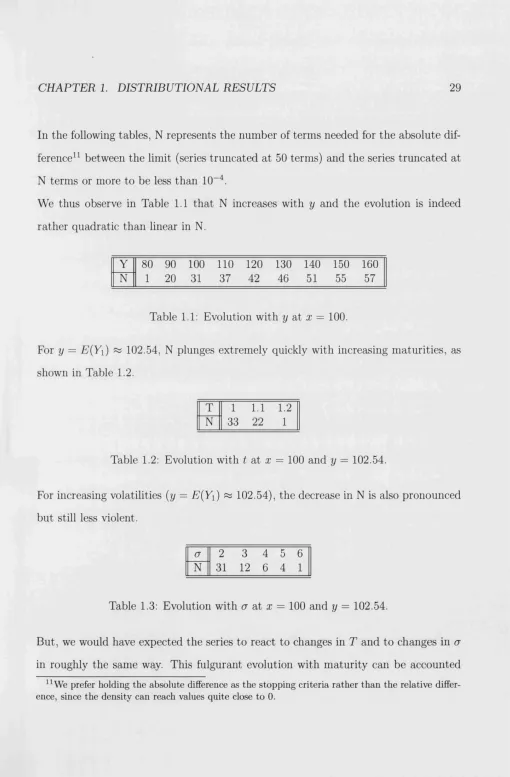
In the following tables, N represents the number of terms needed for the absolute dif
ference^^ between the limit (series truncated at 50 terms) and the series truncated at
N terms or more to be less than 10“^.
We thus observe in Table 1.1 that N increases with y and the evolution is indeed rather quadratic than linear in N.
Y 80 90 100 110 120 130 140 150 160
N 1 20 31 37 42 46 51 55 57
Table 1.1: Evolution with at x = 100.
For y = E{Yi) ^ 102.54, N plunges extremely quickly with increasing maturities, as shown in Table 1.2.
T 1 1.1 1.2
N 33 22 1
Table 1.2: Evolution with ( at x = 100 and y = 102.54.
For increasing volatilities {y = E(Yi) % 102.54), the decrease in N is also pronounced but still less violent.
a 2 3 4 5 6
N 31 12 6 4 1
Table 1.3: Evolution with cr at x = 100 and y = 102.54.
But, we would have expected the series to react to changes in T and to changes in a
in roughly the same way. This fulgurant evolution with m aturity can be accounted
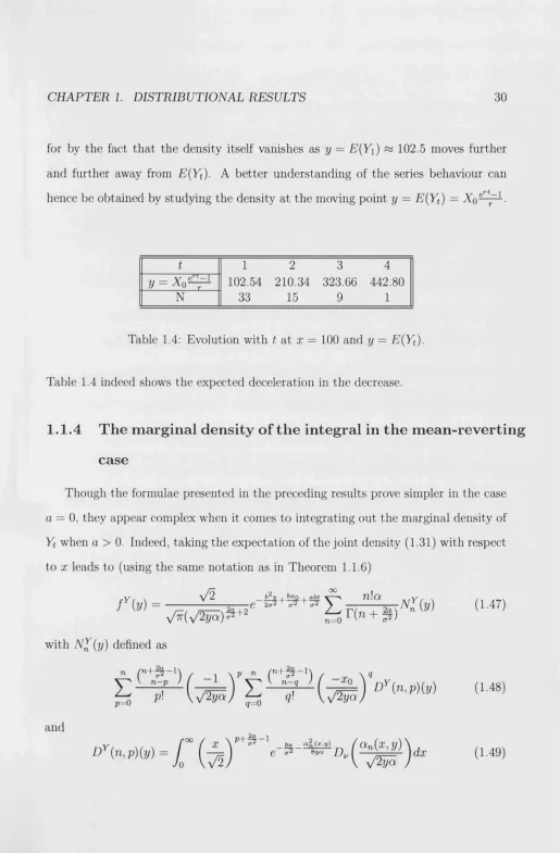
[image:42.595.28.538.31.808.2]CH APTER L D ISTRIBU TIONAL RESU LTS 30
for by the fact th at the density itself vanishes SiS y = E(Yi) % 102.5 moves further and further away from E{Yt). A better understanding of the series behaviour can hence be obtained by studying the density at the moving point y = E(Yt) =
t 1 2 3 4
102.54 210.34 323.66 442.80
N 33 15 9 1
Table 1.4: Evolution with t at x = 100 and y = E{Yt).
Table 1.4 indeed shows the expected deceleration in the decrease.
1.1.4
The marginal density o f th e integral in th e m ean-reverting
case
Though the formulae presented in the preceding results prove simpler in the case
a = 0, they appear complex when it comes to integrating out the marginal density of
Yt when a > 0. Indeed, taking the expectation of the joint density (1.31) with respect to X leads to (using the same notation as in Theorem 1.1.6)
V2 f i y ) — —
y/ïr{^/2ÿâ)^
with (y) defined as rn+%-1
b^yI bxQI abt
E
T ^ r ( n + ^ )n!û; K ( y ) ( 1 . 4 7 )n=0
n y \ p n / _ \ q
and
v / 2 ÿ Q J
[image:43.595.23.538.29.814.2]C H A P T E R !. D ISTRIBU TIO N A L RE SU LTS 31
in which we have altered the notations to an(x, y) to emphasise the dependence on x
and y. Dv{‘) represents the parabolic cylinder function of index v.
Recursions could be used for the D ^(n ,p ){y). Yet, the initial values for those terms would still not be th a t easy to compute and would be needed for each new n.
We thus present here another approach: a direct analytical inversion of the marginal
moment generating function of the integral process, resulting in a tractable and easier
to evaluate formula for its density.
i. R ela tin g th e tw o approaches
Before developing this alternative approach, we first show here how to retrieve
(1.47) by a direct inversion of the marginal MGF of Yt. From (1.1.4),
Decomposing it thanks to the relation (1.46),
Recalling (1.37), the inverse of — fn°° ^ du is12
where the term (3 comes from rescaling the Laplace transform. More precisely.
Inverting (1.51) term by term, we recognise th e terms appearing in (1.47).
C H A P T E R L D ISTRIBU TIO N A L RE SU LTS 32
The sole purpose of this result is to show the consistency of the two approaches
presented in this thesis to compute the marginal density of the integral process. The
marginal MGF can actually be m anipulated in a slightly different manner to lead
to a series representation in which the numerical integration of parabolic cylinder
functions is not required. We will first present a complete formula, in which each
term is explicitly written down, but is - for th a t very reason - unduly complex. The
purpose of this first representation is to show th at it is indeed possible to express
the density in a totally explicit form although in practice, it is more efficient to
evaluate the term s recursively. We therefore present afterwards a reformulation of
this series, constructing its inner terms by recursion. For the square-root process, all
the formulae and applications following this result in the rest of the thesis will be
given in a recursive form. But, it should be kept in mind th a t all of them can be
expressed in a completely explicit manner. For this reason, we call them fully-explicit,
given th a t the really complete series formulation is a straightforward corollary.
ii. T h e c o m p le te fo rm u la fo r t h e d en sity .
D e fin itio n s a n d n o ta tio n s . The density depends on the following functions:
• Hck is the Hermite polynomial (see Appendix A)
[*]
.x^ k\
s=0 ' '
Hck is a polynomial of order k given by (see Appendix A)
[*]
X* k\C H A P T E R 1. D IST R IB U TIO N A L RE SU LTS 33
• For g € N and tu € R+, the function J^„ (y) is defined as
• For I e N and w € R'*', the function is as follows
Case I = 0
J S ,J y ) = (157)
2V7T2/3
Case I = 1
J t M = A W = (1.58)
Case I > 1
/ J e -Ÿ d fi
1-3
T h e o re m 1.1.9. T/ie density o fY t is given by
(j3
defined as in j(1.53))m . ^ e * = s - £k=0 n=0
t s;4= C
\ * - » > * ' “ / "■“ >with
G.,n(y)
=
E '
”) (-1)‘ (
E C)
(-&)*-■
(2/^)
i=0 \ \ j =0
X — W / /
and
j = k —n + l
at + Xq
'^n,i = — ^ ---\-{n + i)t (1.62)
C H A P TE R 1. D ISTRIBU TIO N A L RESU LTS 34
R e m a rk s .
1. The proof of the uniform convergence of the series (1.60) presented in Appendix
1.5.1 is of importance, since it is also applicable for most of the other expansions
derived in the square-root process context. Appendix A also contains recursion for
mulae (see (A.3) and (A.6)) useful to compute numerically the polynomials Hek{x)
and Hek{x).
2. The integrals appearing in (1.59) are only (up to a multiplicative constant) the
complementary error function, which has been widely studied in the literature. There
exists a good number of algorithms to compute it numerically with accuracy, some
of which extremely fast and not taking more th an thrice the time of an exponential
evaluation to get it to machine precision. Most mathem atical software packages have
their own built-in routines to compute it. It can therefore be considered just as
another standard arithm etic function like exp(-) or cos(-) .
(1.60) provides a full analytical expression for f^ { y ) , which enables us to gain a better insight into this density. Yet, as mentioned earlier, employing simplifying
recursions is more efficient than using the explicit formulation of the Gk,n{y), since it cuts down the amount of calculations by an order of magnitude proportional to AT^.
iii. A re c u rs iv e fo rm u la tio n
D e fin itio n s a n d n o ta tio n s . For w G R +\{0}, we construct a sequence Ip,q{'cu) in the following recursive way for positive integers p and q
• For q = 0
C H A P TE R L D ISTR IB U TIO N A L RE SU LTS 35
For q = I
, 2
2 e 4»^ „ I ' — 2yh(3\
For q = 2
,2
- b I „ M (1.65)
• For Ç = 3
= p l { p > 0 } V i , 2 ( l / . r o ) - C T 7 J p , 2 ( j / , r o ) + f ( 1 ^ 6 )
# For q > 3
/ (2/ u ) — "F ‘^yP^p,q-2{y^ '^ip,q-i{y^
Ç - 2
from the only two initial conditions needed:
-—, e
(1.68)
/o,2(y,ti7) = e r f c ( ^ )
R e m a rk s .
1. The term constructed with the previous formulae is either Ip^q or I p + i , q . This differentiation is meant at emphasising whether the formula holds for p = 0 or whether
an initial condition is needed.
2 . The Hermite polynomials appearing in the following recursions are to be them
selves computed by recursion, see Appendix 1.5.1
T h e o re m 1.1.10. The marginal density o f the integral Yt can he rewritten as
= (1.69)
C H A P T E R 1. D IST R IB U T IO N A L RE SU LTS 36
where
nn—n nm <n \ / \ /
n = 0 m = n
and
a t Xq / I \
^ m = — ^ \-m t (1.71)
P ro o f. See Appendix 1.5.2. □
R e m a rk . For programming purposes, it might be simpler to use (with AT > 0, the
number of term s included to compute the series)
=
12
“ M,m4,n(j/,C7m) (1-72) A:=0 m —0 k = m n —k —mk—n
2” (A:—n)! \ ~n ) \ m + n
puted with
where 0 („+"_*) can also be simply recursively
com-(ji — k)(2a {k — n — 1)<7 )
= 2 x o ( m - h n - l - l - A : )
(fc+H)
^0 '^171,0,m
«m+1.0„m+l
-and the initial condition
uo,o,o = 1
iv. N u m e ric a l a p p lic a tio n s
We illustrate the numerical implementation of the series on the set of parame
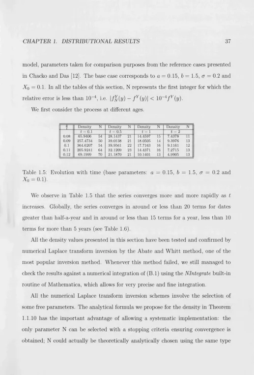
CH APTER 1. D ISTRIBUTIONAL RESULTS 37
model, parameters taken for comparison purposes from the reference cases presented
in Chacko and Das [12]. The base case corresponds to a = 0.15, b = 1.5, cr = 0.2 and %o = 0.1. In all the tables of this section, N represents the first integer for which the
relative error is less than 10“"^, i.e. |/^(?/) - f ' ^ { y ) \ < 10~^/^(r/). We first consider the process at different ages.
— 2
-t Density N Density N Density N Density N
t = 0.1 t = 0.5 t = 1 f = 2
0.08 65.9406 54 28.1437 21 14.4597 15 7.4378 11
0.09 257.4734 50 39.0138 21 18.0505 14 9.3976 13
0.1 364.6207 54 39.9561 22 17.7163 16 9.1161 12
0.11 205.9241 64 32.1209 23 14.4371 16 7.2715 13
0.12 69.1999 70 21.1870 21 10.1401 13 4.9905 13
Table 1.5: Evolution with time (base parameters: a = 0.15, b = 1.5, a = 0.2 and
X q = 0.1).
We observe in Table 1.5 that the series converges more and more rapidly as t
increases. Globally, the series converges in around or less than 20 terms for dates
greater than half-a-year and in around or less than 15 terms for a year, less than 10
terms for more than 5 years (see Table 1.6).
All the density values presented in this section have been tested and confirmed by
numerical Laplace transform inversion by the Abate and W hitt method, one of the
most popular inversion method. Whenever this method failed, we still managed to
check the results against a numerical integration of (B.l) using the NIntegmte built-in routine of Mathematica, which allows for very precise and fine integration.
All the numerical Laplace transform inversion schemes involve the selection of
some free parameters. The analytical formula we propose for